
Run-Length-Based River Skeleton Line Extraction from High-Resolution Remote Sensed Image


1
College of Civil Engineering and Architecture, Zhejiang University, Hangzhou 310058, China
2
Zhejiang Institute of Hydraulics & Estuary (Zhejiang Institute of Marine Planning and Design), Hangzhou 310020, China
3
Key Laboratory for Geographical Process Analysis & Simulation of Hubei Province, Central China Normal University, Wuhan 430079, China
4
College of Urban and Environmental Sciences, Central China Normal University, Wuhan 430079, China
5
Jiangsu Provincial Planning and Design Group, Nanjing 210019, China
6
Changjiang River Scientific Research Institute, Changjiang Water Resources Commission, Wuhan 430010, China
*
Author to whom correspondence should be addressed.
Remote Sens. 2022, 14(22), 5852; https://0-doi-org.brum.beds.ac.uk/10.3390/rs14225852
Submission received: 6 October 2022
/
Revised: 7 November 2022
/
Accepted: 14 November 2022
/
Published: 18 November 2022
(This article belongs to the Special Issue Monitoring Terrestrial Water Resource Using Multiple Satellite Sensors)
Abstract
:Automatic extraction of the skeleton lines of river systems from high-resolution remote-sensing images has great significance for surveying and managing water resources. A large number of existing methods for the automatic extraction of skeleton lines from raster images are primarily used for simple graphs and images (e.g., fingerprint, text, and character recognition). These methods generally are memory intensive and have low computational efficiency. These shortcomings preclude their direct use in the extraction of skeleton lines from large volumes of high-resolution remote-sensing images. In this study, we developed a method to extract river skeleton lines based entirely on run-length encoding. This method attempts to replace direct raster encoding with run-length encoding for storing river data, which can considerably compress raster data. A run-length boundary tracing strategy is used instead of complete raster matrix traversal to quickly determine redundant pixels, thereby significantly improving the computational efficiency. An experiment was performed using a 0.5 m-resolution remote-sensing image of Yiwu city in the Chinese province of Zhejiang. Raster data for the rivers in Yiwu were obtained using both the DeepLabv3+ deep learning model and the conventional visual interpretation method. Subsequently, the proposed method was used to extract the skeleton lines of the rivers in Yiwu. To compare the proposed method with the classical raster-based skeleton line extraction algorithm developed by Zhang and Suen in terms of memory consumption and computational efficiency, the visually interpreted river data were used to generate skeleton lines at different raster resolutions. The results showed that the proposed method consumed less than 1% of the memory consumed by the classical method and was over 10 times more computationally efficient. This finding suggests that the proposed method has the potential for river skeleton line extraction from terabyte-scale remote-sensing image data on personal computers.
1. Introduction
River data are the most important basic data in the fields of hydrology and water resources research. In the context of river systems, a hydrographic network often refers to a river with a branched structure comprising a mainstream and several tributaries interconnected within a basin, while a river network refers to a river with a network structure formed by multiple rivers interconnected in a plain area [1]. The skeleton lines of rivers are an abstract description of their shape and generally refer to the curves at their center that reflect their main extension direction and shape characteristics [2]. River skeleton line extraction is required in numerous application scenarios. For example, dual-line rivers are often simplified as single-line rivers in the thematic mapping of water resources [2]. Skeleton line extraction is also required to detect and identify rivers from remote-sensing (RS) images [3,4,5]. Moreover, river skeleton lines have great application significance as a reference for applications such as water resource monitoring, land planning, and ship-based transportation [6]. In many provinces of China, such as Zhejiang Province, provincial water area surveys are carried out every few years. The basic information and spatial data of rivers, lakes, reservoirs, mountain ponds, artificial waterways, flood storage and detention areas, and other water areas in the province were comprehensively identified and mapped using technologies such as aerospace remote sensing, geographic mapping information, the Internet and big data, so as to clarify the specific scope of water area protection and shoreline control, and delineate the “three lines” space of water surface line, shoreline and water area management scope line. The skeleton line of the river system is one of the basic information of the water area to be extracted.
Rapid advances in RS technology have enabled the identification of water bodies from RS images to become the most important means to acquire river data. Methods commonly used to obtain river data from RS images include the conventional visual interpretation method, spectral feature methods (e.g., single-band threshold, multi-band threshold, and water-body index methods) [7,8], classifier methods (e.g., support vector machine, object-oriented, and decision-tree methods) [9], and deep-learning (DL) artificial intelligence algorithms (currently the most popular methods) [10,11]. These methods can be used to directly obtain river data in a binary raster format, from which specific raster algorithms can be employed to extract river skeleton lines.
A multitude of methods have been developed to extract skeleton lines from raster images, which can be grouped based on the design principle into two categories: non-iterative and iterative algorithms. Common non-iterative algorithms include central-axis transformation [12], surface clustering [13], thermodynamic equations [14], cellular automata [15], mathematical morphology [6], and neural network models [16]. Iterative algorithms mainly include the classical raster thinning algorithm [17] and its improved variants [18,19,20]. Currently, the classical raster thinning method developed by Zhang and Suen (1984) is recognized as a relatively mature method and is the most widely used. This method is a multi-iteration shrinkage algorithm that gradually removes the boundary points or reduces the unnecessary points from a raster until advancing to its interior to extract the skeleton line while maintaining the topological invariability of the polygon.
Owing to their simple program design and ease of parallelization [21], raster-based skeleton line generation methods have been applied extensively in the fields of image processing and virtual simulation [13,14], such as fingerprint recognition [16], text and character recognition [22,23], and 2.5- and 3-dimensional vision [12]. A raster image is, in essence, matrix-based direct raster-encoded data, the volume of which increases exponentially as the number of rows and columns in the grid increases. Previous researchers often used various simple cartoon images in their investigation of skeleton line extraction [14] while giving little consideration to the volume of raster data. For example, Mahmoudi et al. [24] used images containing only 512 rows and 512 columns in their study. RS images are characterized by high resolution and large data volume. The spatial resolution of RS images can easily reach 1 m or even the sub-meter level. Conventional raster-based skeleton line extraction methods are susceptible to computational failure due to computer memory limitations. Here, the river system in an area with a size of 100 × 100 km is used as an example. Assuming that the spatial resolution of the RS image of the area is 0.5 m and that each grid cell stores 1 B of data, if all the data are read into the memory, the raster data volume can reach 37.25 GB, which is a heavy burden for a personal computer. The extraction of the skeleton lines of the river system in the Yangtze River basin in China is a more representative case. Because the Yangtze River basin spans 6000 km from east to west and 4000 km from north to south, the data volume can reach 223 GB even when calculated based on a raster resolution of 10 m. In contrast, unlike block cartoon images, the high spatial resolution of RS images means that finer information on the mainstreams and tributaries of rivers can be obtained. The extraction of the skeleton lines of these types of long and narrow rivers with a large number of tributaries has always been a challenge in skeleton line extraction research [25].
The various reasons presented above preclude the use of conventional raster-based skeleton line extraction methods to achieve high accuracy and efficiency in the extraction of river skeleton lines from RS images of large areas. For example, Meng et al. [6] used the Rosenfeld algorithm [26] to extract river skeleton lines from RS images with a spatial resolution of only 16 m that only covered partial sections of the Li River basin. In the study by Guo et al. [4], the study area was limited to the area shown in a single aerial photograph. As a result, only the skeleton lines of the sections of the river in a local area could be extracted. Hence, in this study, based on the approach of Zhang and Suen’s classical raster method, we propose to compress raster data for rivers using run-length encoding (RLE) with consideration for the presence of extensive data redundancy in binary raster images of rivers, as well as provide a solution for the efficient extraction of river skeleton lines based entirely on run-length-encoded data.
2. Methods
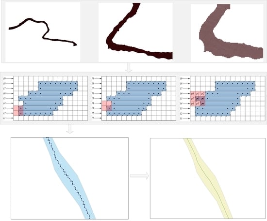
Figure 1 shows the process of extracting river skeleton lines from an RS image. First, raster data for the river system are extracted from the RS image. Subsequently, the raster data for the river are converted to run-length-encoded data using the proposed run-length method. In addition, raster data for the river skeleton lines are automatically generated through run-length boundary tracing in conjunction with iterative calculations integrated with pixel removal. Finally, the raster is automatically vectorized to generate vector line data for the river skeleton lines (Section 2.4). The key steps are elaborated on in the following sections.
2.1. Extraction of Raster Data for a River System from an RS Image
Conventional methods based on the spectral signatures of RS images establish models for single or multiple image bands. They focus more on the calculation of pixel values and less on other spatial features (e.g., image texture). Although they are simple and easy to implement, these methods tend to identify shadows or buildings as water bodies, which considerably limits the extraction accuracy for water bodies. The classifier approach designs classifiers for image features and extracts water bodies based on specific algorithmic rules and, therefore, can somewhat eliminate the effects of shadows and buildings. However, in this approach, feature extraction and classifier design depend on expert knowledge. In addition, classifiers are not versatile for different regions and effects [27].
In recent years, DL has provided an effective framework for the classification and recognition of massive RS image data, gradually advancing RS image processing. Moreover, DL has achieved marked progress in object detection, image classification, and parameter extraction. In this study, an attempt was made to use the DeepLabv3+ model to extract river data from a high-resolution RS image. The DeepLabv3+ model is a DL model for semantic image segmentation and is the latest improved version in the DeepLab series of models developed by the Google research team. The most significant contribution of the DeepLab series of models to semantic image segmentation is the development of dilated convolution and a series of subsequent improvements [28]. The latest DeepLab model (i.e., DeepLabv3+) has the following advantages: more shallow information is retained in the model network based on the feature fusion strategy for object detection; the edge detection accuracy is optimized by exploiting the advantages of the encoder–decoder architecture and Atrous Spatial Pyramid Pooling, as well as gradually recovering spatial information to capture clear object boundaries; and depth-wise separable convolution is also added to optimize the performance of the segmentation network. When tested on the PASCAL Visual Object Classes 2012 dataset, the accuracy of the DeepLabv3+ network exceeded the then-highest level. The DeepLabv3+ network is one of the most mature semantic segmentation networks currently available. Figure 2 shows the architecture of the DeepLabv3+ DL model [29].
DL models are effective in extracting permanent water bodies (e.g., large rivers). Small streams and man-made waterways are known for their complex changes and seasonal and intermittent drying-up periods; therefore, it is difficult to extract continuous, uninterrupted water bodies using DL models. Hence, in this study, a more complete set of river-system data was additionally extracted from the RS image through visual interpretation. This task was completed primarily through direct manual extraction of the river boundaries using ArcGIS software. First, load the remote sensing image into ArcGIS software. Second, create a new river vector layer and visually sketch all rivers and their branches on the remote sensing image. Third, use the “Extract by Mask” in ArcToolbox to cut the sketched river water body vector data and remote sensing image to obtain remote sensing data that only retains river water bodies. Finally, the remote sensing data of river water body is converted into binary raster data.
2.2. Conversion of Raster Data to Run-Length-Encoded Data for Rivers
River data generated by a DL model and visual interpretation are direct raster-encoded data. Reading these data simultaneously is a memory-intensive process for a personal computer. To address this issue, raster-encoded river data can be read blockwise based on strips and compressed in real-time through RLE [30]. RLE is a typical raster data compression method [31] that is particularly suitable for compressing binary images [32,33]; only two values—the values of the starting and ending columns of non-zero-pixel values in a raster row—are required to be stored in a run length.
Compared with conventional raster-based skeleton line generation methods, the proposed method does not store raster-encoded data in matrix format in the computer memory but instead directly stores run-length-encoded data in list format. Table 1 summarizes the run-length and run-length list structures in a raster row expressed using the C language. A single run length is expressed using struct “Runlength” that stores its starting column number “StartColNo” and ending column number “EndColNo” along with a pointer to the next (right) run length, “NextRunlength”. A run-length list, “RunlengthLIST”, is created for each row in the raster field. The run-length list stores the number of run lengths, “RunlengthNum”, in the row along with the pointer to the first run length from the left, “FirstRunlength”.
Figure 3 shows a schematic diagram of the conversion of direct raster-encoded data to run-length-encoded data for a river section (the red grid cells are the target pixels representing the river [value = 1], and the white grid cells are the background pixels [value = 0]). Direct raster encoding stores a matrix comprising 9 rows and 15 columns and needs to store a total of 135 values for the whole river data. If the data are stored in RLE format, no values need to be stored for the non-river area, and only the run-length information for the river in each row of the raster field needs to be marked. As shown in Figure 3, seven run lengths are generated in the graph, which are located in rows l2 and l8. For example, run length (2, 8) is stored in row l2. A total of seven run lengths (14 values) need to be stored for the whole raster field. Compared to direct raster encoding, RLE compresses data at a ratio of 89%.
2.3. River Skeleton Line Generation Based on RLE
2.3.1. Rules for Determining Redundant Pixels
Based on the rules used by Zhang and Suen to determine pixel connectivity, redundant pixels are gradually eliminated from an image through multiple iterations. In a single iteration, the preset rules are used to determine the redundant pixels that need to be removed. As shown in Figure 4a, p1, p2, p3, p4, p5, p6, p7, and p8 are the eight pixels adjacent to pixel p0. The basic relationship between any two adjacent pixels is defined below:
where w is a value in the range of 1–8. In particular, when w = 8, because p9 does not exist, the relationship between p8 and p1 should be examined. In other words, when p8 = 0 and p1 = 1, . The sum of the relationships of pixel p0 with all of its adjacent pixels is given below:
As shown in Equations (3) and (4), and are the rules for determining the connectivity of pixel p0. If p0 = 1 and = 1 or = 1, then p0 is a redundant pixel and can be directly removed (p0 is set to 0):
In direct raster encoding, a pixel value is stored as a two-dimensional (2D) array. Therefore, to determine whether a pixel is redundant, an operation can be directly performed on the 2D array to access the values of the eight adjacent pixels. Operations on run-length-encoded data are more complex. As shown in Figure 4b, to determine the connectivity of pixel p0, the run-length list needs to be first searched sequentially in row l5 to find whether pixel p0 is located in the run lengths. To access the values of the eight pixels adjacent to pixel p0, the run-length lists in the rows above and below l5 also need to be searched.
2.3.2. Run-Length Boundary Tracing and Redundant Pixel Removal
In the classical raster method developed by Zhang and Suen (1984), all pixels need to traverse twice in one iteration. During the first traversal, a set of pixels that need to be removed is determined based on Equation (3). After the removal of these pixels, the second traversal begins, during which a set of pixels that need to be removed is determined based on Equation (4). After the removal of the pixels, the algorithm begins another iteration. Finally, the iterative calculation process is terminated when there are no more removable pixels. The remaining target pixels constitute the skeleton lines of the image.
As shown in the above analysis, determining the connectivity of all the pixels using the above approach can inevitably gravely affect the computational efficiency in RLE. Considering that removable pixels only appear at the boundaries of a graph in one iteration of the calculation, the connectivity of the pixels located in the interior of the graph does not need to be determined. As shown in Figure 5, an efficient strategy is to trace along the boundary of the set of run lengths to search all the boundary pixels (the pixels labeled with black dots in Figure 5). Therefore, only the connectivity of the boundary pixels needs to be determined. This method turns the determination of redundant pixels from a line-by-line and pixel-by-pixel process to a run-length boundary tracing process, thus cleverly removing redundant pixels at the boundary. As shown in Figure 5, only 35 boundary pixels need to be determined if they are redundant in the first iteration, compared with 57 pixels in the original process. This translates to a 38% decrease in the computational load.
2.3.3. Design of Boundary Tracing Direction Templates
A real-world river system may contain an island structure, resulting in multiple boundaries. In Figure 6, the red and blue lines are the outer and inner boundaries of the river, respectively. Run-length boundary tracing may occur on either the outer or inner boundary of the river. In Figure 5, arrows are used to indicate the run-length boundary tracing directions. There are four directions: up, down, left, and right. Setting a reasonable run-length boundary tracing rule is crucial as it determines whether run-length boundary tracing can form a closed loop (i.e., return to the starting edge). Hence, for rivers with complex inner and outer boundaries, templates for determining the run-length boundary tracing direction were developed in this study.
As shown in Figure 7, a 2 × 2 window is used to search along the run-length boundary to locate all of the boundary pixels and determine whether they are redundant. There are a total of 24 scenarios for the determination of the run-length boundary tracing direction. The first three columns (from the left) show the scenarios of the tracing of the outer boundary of an image, and the last three columns show the scenarios of the tracing of the inner boundary of an image.
During each iteration of the calculation, run lengths are searched row by row, starting from the bottommost row and moving up. When the left (right) side of a run length is found untraced, it is used as the starting tracing edge, with the tracing direction marked as “up”. This step is followed by boundary tracing and determination of the connectivity of the boundary pixels while ensuring that the left and right sides of each run length are traced. If the left side of a run length is the starting tracing edge, it means that tracing occurs on the outer boundary of the river. Conversely, if the right side of a run length is the starting tracing edge, it means that tracing occurs on the inner boundary of the river. In the set of run lengths in Figure 5, the left side of the run length in row l2 is the starting tracing edge. Figure 8a,b shows the first two steps of determination of the tracing direction for the left side of the run length in row l2 based on a 2 × 2 window, which uses the “up to up” and “up to right” templates in the second row in Figure 7, respectively.
2.4. Vectorization of River Skeleton Lines
After the removal of the redundant pixels, all the run lengths in the raster field constitute river skeleton lines. The points in Figure 9 represent the pixels where the skeleton lines are located. The extraction of skeleton lines from run lengths refers to the automatic generation of skeleton lines based on the order in which pixels are stored after they are located sequentially based on their adjacency. Analysis of the pixels comprising the skeleton lines reveals that these pixels can be grouped into three categories, namely, endpoint pixels, junction pixels, and bifurcation pixels. An endpoint pixel refers to a pixel at which skeleton line tracing starts or ends (starting or ending pixels, respectively). There is only one target pixel among the eight pixels adjacent to an endpoint pixel. If such a pixel has already been searched, the endpoint pixel is an ending pixel; otherwise, the endpoint pixel is a starting pixel, as shown in Figure 10a. Junction pixels refer to the pixels that act as connections in skeleton lines. Among the eight pixels adjacent to a junction pixel, there is only one unsearched pixel, or there are two adjacent pixels, as shown in Figure 10b. Bifurcation pixels refer to points at which multiple branches occur in skeleton lines. An unsearched pixel has two nonadjacent target pixels, resulting in a bifurcation, as shown in Figure 10c.
In this study, considering the complex characteristics (e.g., bifurcations) of rivers, searching is terminated at each bifurcation pixel during the extraction of skeleton lines, followed by the generation of three skeleton lines from the bifurcation pixel. In Figure 10a, the red pixels are pixels that are currently searched. Among the eight pixels adjacent to each red pixel in Figure 10a, if there is only one target pixel and it has not been searched, then this pixel is to be searched next; otherwise, this pixel is the ending pixel of a skeleton line. As shown in Figure 10b, junction pixels can be divided into two categories: pixels with only one adjacent pixel that is unsearched and is to be searched next and pixels with two adjacent pixels (out of a total of eight) that are unsearched and adjacent to each other. If there is more than one unsearched adjacent pixel, the pixel above is searched next, followed by the pixel to the right, the pixel below, and the pixel to the left. As shown in Figure 10c, searching is terminated if two unsearched pixels that are not adjacent to each other are found among the pixels adjacent to the pixel that is being searched currently. Each time a pixel is searched, this pixel is removed from the run length until no run length can be found in the run-length list, which means that all the skeleton lines are extracted. The skeleton lines obtained from tracing are jagged line segments with a large number of redundant pixels; they can be smoothed using software such as ArcGIS.
3. Study Area and Data Set
Located in the city of Jinhua in the Chinese province of Zhejiang, the city of Yiwu (119°49′–120°17′ E; 29°2′–29°33′ N) (as shown in Figure 11) spans 58.15 km from north to south and 44.41 km east to west, and encompasses a total land area of 1105 km2. Yiwu has a river system composed of intertwined natural and man-made rivers that vary dramatically in width, which is typical in southern China. There are five types of water bodies in Yiwu, namely, rivers, reservoirs, mountain ponds, man-made waterways, and other water bodies, which collectively cover an area of 52.17 km2. This means that 4.72% of the ground surface in Yiwu is covered with water. The Yiwu River is the longest mainstream river in Yiwu, crossing the city from west to east over a distance of 40 km. Figure 11 shows the high-resolution satellite RS image provided by Yiwu Natural Resources and Planning Bureau used in this study, with a spatial resolution of 0.5 m and 116,326 rows and 90,801 columns in the grid.
In this study, the DeepLabv3+ DL model was used to extract data for the water bodies across Yiwu. A small portion of the data for the river system in Yiwu collected in this study was rasterized to create a raster image of the real water bodies at a resolution consistent with that of the RS image. A raster grid with 1024 × 1024 cells was used to crop the RS image and the raster image of the real water bodies. Ultimately, in total, 982 DL samples were obtained to form a sample set for the DeepLabv3+-based DL model for water-body extraction. Based on the general training and testing requirements for DL models, the DL sample set was divided into a training set, a validation set, and a test set at a ratio of 8:1:1 to train and test the Deeplabv3+-based DL model for water-body extraction. The three types of samples were divided randomly based on their ordinal numbers to allow the samples with different roles to be evenly distributed in space. Figure 12 shows the spatial distribution of the sample set in the study area.
The DeepLabv3+ model was trained to distinguish between water bodies and non-water bodies in the image on the prepared DL training set. Cross entropy (CE) was used as the loss function of the model to optimize the grid parameters. Specifically, CE was primarily employed to describe the difference between the predictions yielded by the model and the reality and guide the DL model to reduce its error. In this study, the DL model was trained 100 times, each of which involved four samples. After each time of training, the training accuracy was examined using the samples in the validation set. As shown in Figure 13, two metrics, intersection-over-union (IoU) and accuracy (ACC) were used to evaluate the capacity of the model to distinguish water bodies during training. IoU refers to the ratio of the categories correctly extracted by the model to the union of the categories output by the model and the real categories. In Figure 13b, the orange line represents the IoU of the non-water body and the gray line represents the IoU of the water body. ACC refers to the proportion of the pixels that are correctly identified. Figure 13a–c shows the training results for the DeepLabv3+ model.
The actual capacity of the trained DeepLabv3+ model to extract water bodies was tested using the samples in the test set. The model was used to produce a prediction for each sample, which was compared with the reality. IoU and ACC were used as the comparison metrics. Table 2 summarizes the test results.
The test results showed that the model correctly identified more than 97% of the pixels, suggesting that the DeepLabv3+-based water-body extraction model was sufficiently accurate for extracting water bodies from the RS image in this study. Figure 14 shows the Yiwu water-body (partial) data extracted by the trained Deeplabv3+ DL model from the image of the entire city of Yiwu. The extracted water-body raster image was vectorized and checked using topology rules in ArcGIS. Conspicuously erroneous water bodies (e.g., damaged and incomplete water bodies) were removed. Thus, a total of 9458 water-body elements were extracted, covering a total area of 55 km2.
The data generated by the Deeplabv3+ DL model consisted of all the water-body elements in Yiwu. However, most of the water bodies are not rivers. Therefore, only the mainstream of the Yiwu River and its major tributaries were retained in this study to generate raster data for the major rivers in Yiwu, as shown in Figure 15a. The raster data for the rivers in Figure 15a had a resolution consistent with that of the RS image and contained 91,460 rows and 69,586 columns in the grid. Many tributaries of the Yiwu River are small streams that dry up seasonally and intermittently. Identifying narrow, long, continuous rivers on RS images is a challenging task. Therefore, to obtain relatively complete data for the mainstream and major tributaries of the Yiwu River, the rivers were outlined through visual interpretation, as shown in Figure 15b. This set of raster data contained 74,170 rows and 58,234 columns.
4. Results and Analysis
4.1. Analysis of the Extracted Skeleton Lines
Based on the proposed run-length-based skeleton line extraction method, the program automatically reads two sets of raster river data. The data were read blockwise and compressed once to directly generate run-length-encoded river data in the computer memory. Thus, skeleton line data for the Yiwu River system were obtained. Figure 16a shows the visually interpolated river data, the generated skeleton lines, and the corresponding pixels. Figure 16b shows the river data generated by the DL model, the generated skeleton lines, and the corresponding pixels. It is evident that the skeleton line pixels with a resolution of 0.5 m can satisfactorily indicate the central axis of the river and the direction of its branches.
As shown in Figure 17a, the skeleton line can satisfactorily characterize the direction of a single river with gentle changes in direction and width; however, natural river systems have complex characteristics such as numerous bifurcations. Therefore, researchers are concerned regarding whether the generated skeleton lines preserve the bifurcation characteristics of rivers. Figure 17b shows the bifurcations of the Yiwu River in a local area. At each bifurcation, the width of the mainstream differs markedly from that of the branch. The skeleton lines of the mainstream and branches satisfactorily show the characteristic bifurcations of the river. Furthermore, rivers are often connected to other water bodies (e.g., lakes, reservoirs, and ponds), resulting in sudden changes in their direction and an abrupt increase in their width. As shown in Figure 17c, the proposed method was also effective in extracting satisfactory skeletal lines from water bodies (e.g., lakes, reservoirs, and ponds), which led to an increase in the width of the river. The skeleton lines also satisfactorily connected the river sections upstream and downstream of the lakes, reservoirs, and ponds and remained continuous. Figure 17d shows an example where the river bifurcates, and the branches converge later. This is a common island structure in rivers. The bifurcation and convergence characteristics of the river were retained in the skeleton lines generated using the proposed method.
4.2. Skeleton Line Extraction Performance Analysis
In general, the run-length method is, in essence, a special raster method, the performance of which is still affected by the spatial resolution of the image and the number of rows and columns in the raster image. To analyze its application potential in dealing with large volumes of data, the proposed run-length method was compared with the algorithm developed by Zhang and Suen using the C# development language on a computer equipped with an Intel® CoreTM i7-10750H central processing unit at 2.60 GHz and 32.00 GB of memory and running on a 64-bit Windows 11 operating system.
First, the sweep-line algorithm was used to convert the vectorized river boundaries outlined by visual interpretation to raster data with different spatial resolutions [34,35]. Because the sweep-line algorithm can directly read the river-boundary vector data and subsequently complete RLE memory compression [30], generating raster image files with different spatial resolutions in advance is not required. A statistical analysis of memory consumption revealed the following: Zhang and Suen’s method required the construction of two 2D sets of data—one for storing the raster river data and the other for marking whether pixels should be removed. Therefore, each grid cell was required to store 2 B of data. The proposed method uses a List object in the C# language to store the run-length list. Each run length stored the values of the starting and ending columns which amounted to a total of 8 B. As shown in Table 3, 11 tests were conducted based on different spatial resolutions, in which the grid cell width was gradually refined from 10 to 0.1 m. The computational time and memory usage were determined for Zhang and Suen’s method and the run-length method. In Table 3, “Time” is the total time taken to execute the core algorithms, and “Total memory” is the total memory allocated to the direct raster-encoded and run-length-encoded river data during the execution of the algorithms. At a grid cell size of 0.6 m, Zhang and Suen’s method failed because the computer was unable to allocate a large 2D array.
- (1)
- Computational efficiency. It is evident from Table 3 that the run-length method was superior in terms of computational efficiency. At a grid cell size of 1 m, the run-length method still took only approximately 3 min to complete the computation, compared to more than 30 min for Zhang and Suen’s method. A data comparison revealed that the ratio of the time consumed by Zhang and Suen’s method to the time consumed by the run-length method increased rapidly as the grid cell size decreased. As the grid cell size was refined to 0.1 m, the number of rows and columns in the grid reached the order of hundreds of thousands. Under this condition, the proposed method still exhibited excellent stability.
- (2)
- Memory consumption. In the extraction of the skeleton lines of a bifurcated river, the memory to be allocated is related to the complexity of the bifurcated river in addition to the raster resolution. The more complexly the river is bifurcated, the more run lengths there are in the raster rows, and the more memory is required. However, the run-length method can completely deal with all types of complex river data, with almost no requirement to consider memory limitations. As seen in Table 3, even if the spatial resolution was set to 0.1 m, which increased the number of rows and columns in the grid to 300,000, less than 20 MB of memory was used to store the run-length data. At a resolution of 0.1 m, Zhang and Suen’s method required 215 GB of memory. The run-length method is hugely advantageous in terms of memory consumption and can theoretically handle terabyte-scale raster data.
5. Discussion
The proposed run-length method is consistent with Zhang and Suen’s method in terms of the rules for determining redundant pixels. Accordingly, the boundary morphology of a river has a marked impact on the extraction of its skeleton lines. As shown in Figure 18, compared to the DL model (Figure 18a), visual interpretation (Figure 18b) yielded a continuous river with smoother boundaries and generated skeleton lines with a smoother course and fewer bends. In contrast, as shown in Figure 18a, the skeleton lines generated by the DL model contained a large number of unnecessary branches (red box (3) in Figure 18a) that require removal through post-processing treatments. In addition, a breakup in the river led to a ruptured skeleton line with two parts that needed to be connected (red boxes (1) and (2) in Figure 18a). Meng et al. [6] developed a method to automatically connect ruptured skeleton lines based on mathematical morphology and topology constraints. Similar problems will also be encountered in the research of road centerline extraction. Yuan and Xu [36] proposed a Loss Function (GapLoss) method for the Semantic Segmentation of roads, which can well solve the problem of road route fracture. Overall, the skeleton lines generated from the visually interpreted river data were finer and required fewer post-processing treatments.
The raster resolution has a significant impact on the extraction of skeleton lines. The higher the raster resolution (i.e., the smaller the grid cell size), the finer the skeleton lines. In addition, it is imperative to ensure that the grid cell size is smaller than the river width; otherwise, the river is unable to cover a grid cell, resulting in seriously distorted skeleton lines. Figure 19 compares the skeleton lines extracted at grid cell sizes of 10, 2, and 0.1 m. It is evident that the skeleton lines extracted at a resolution of 0.1 m were appreciably better than those extracted at resolutions of 10 and 2 m. As shown in Figure 19a, at a raster resolution of 10 m, part of the river could not completely occupy a single grid cell. Consequently, part of the water body was marked as background pixels, and the generated skeleton lines were composed of broken lines. For a large river system with many tributaries, the effect of skeleton line extraction depends not on the main river but on the tributaries with complex structures. Because the mainstream and tributary are at the same raster resolution, while the river width of the tributary is narrower, in order to obtain a good extraction result, the requirements for raster resolution will be higher, and the focus should be on the river width of the tributary. The comparative test analysis in this study revealed that a grid cell width of one-tenth of the river width can ensure that the generated river skeleton lines are of good fidelity. Visual interpretation revealed a general width of approximately 5 m for the narrowest portions of the mainstream and tributaries of the Yiwu River. Therefore, the 0.5 m-resolution raster data for the river obtained through visual interpretation and the DL model generally met the requirements.
It is also a feasible method to extract river skeleton lines from the perspective of a vector algorithm. Through triangulation of river polygons, the midpoints on the edges are reasonably extracted from the triangles, and these midpoints are connected in sequence with complex design strategies to generate skeleton lines. Lewandowicz et al. [37] proposed a Base Point Split (BPSplit) algorithm for extracting lake skeleton lines. Compared with the raster method, the vector method does not care much about the accuracy of skeleton lines, but the implementation of the vector algorithm is generally too complex. In the vector algorithm, it is necessary to deal with the complex polygon holes, provide a feasible solution, and reasonably design to accurately trace the skeleton line from the triangles [38,39,40]. In addition, some pre-processing operations are difficult to avoid. For example, Lewandowicz’s method [36] needs to select all the base points at the entrance and exit of the lake. Some software, such as ArcGIS, also provides similar centerline extraction tools [41], but it is susceptible to graphics boundaries. The vector boundaries on both sides of the centerline must have certain parallel features.
At present, the resolution of remote sensing image data has been greatly improved. Remote sensing data with sub-meter resolution has been particularly common. Under this resolution, it is almost unnecessary to pay too much attention to the accuracy of river skeleton lines. As shown in Table 3, multiple resolution data (10 m~0.6 m) are simplified from the original resolution data (0.5 m). The proposed method can deal with a large number of raster images without considering the limitation of computer memory.
Run-length-encoded data are still a special type of raster data that can be easily parallelized. The case examined in this study, in which the raster field is divided into strips, is used as an example. For example, a raster field with 10,000 rows can be automatically divided into five strips (each containing 2000 rows) for parallelization. Outward expansion by a few rows of raster cells from the strip boundaries alone can allow for the skeleton lines generated from the calculation of each strip to be connected.
Figure 20a shows a river polygon and its run-length data; the entire raster field is divided into 20 rows. If the raster field is divided into two blocks, rows 1–10 are divided into the lower block and rows 11–20 are divided into the upper blocks. Figure 20b,c are schematic diagrams of the upper block and lower block run-length boundary tracing. In a parallel environment, the boundary tracing of two blocks is carried out synchronously; that is, the lower block starts to traverse the run from line 1 until line 10 stops, and the upper block starts to traverse the run from line 11 until line 20 stops. When tracing to the block boundary, adjacent blocks will not be entered. For an independent river polygon, after each block completes boundary tracing, delete redundant pixels at one time and then start block tracing again.
6. Conclusions
This study presents a method to generate skeleton lines for complex river systems based on RLE. The method can address the problem associated with common raster methods—they are unable to handle large volumes of raster river data generated from high-resolution RS data—and has the two advantages of low memory consumption and high computational efficiency. Skeleton line extraction is required for graphical data (e.g., for road networks and river systems) and also has a wide range of applications in image processing. As demonstrated, the proposed run-length-based skeleton line extraction method can be used for river systems; however, it can also be extended to generate skeleton lines for buildings, road networks, and images. The main work of this study is summarized as follows:
- (1)
- An RLE structure for storing large-scale river raster data is proposed, which can compress the amount of raster data to less than 1%. The link list structure is particularly suitable for representing complex river systems with islands.
- (2)
- A river boundary pixel deletion strategy based on RLE data is designed, which is implemented by using run length boundary tracing iteration operation and provides a template for judging the direction of boundary tracing.
- (3)
- A method of vectorizing skeleton lines from RLE data with skeleton line pixels only reserved is designed. By identifying endpoints, junctions, and bifurcation, skeleton lines are automatically reorganized.
Zhang and Suen’s research gives a complete method of generating skeleton lines from binary grid images and also gives its parallel implementation scheme. This study only compares the proposed method with Zhang and Suen’s method in the non-parallelization case. Follow-up studies will be focused on further improving the run-length algorithm in terms of its parallelization capabilities to enhance its application potential when dealing with massive volumes of RS data.
Author Contributions
H.W. and D.S. conducted the primary experiments, cartography, and analyzed the results. D.T. provided the original idea for this paper. W.C., Y.L. and Y.X. actively participated throughout the research process and offered data support for this work. All authors have read and agreed to the published version of the manuscript.
Funding
This research was supported by the Water Science and Technology Plan of Zhejiang Province (RC2104) and the Fundamental Research Funds for the Central Universities (CCNU22QN019), funded by Department of Water Resources of Zhejiang Province and Central China Normal University, respectively.
Acknowledgments
We would like to express appreciation to our colleagues in the laboratory for their constructive suggestions. Moreover, we thank the anonymous reviewers and members of the editorial team for their constructive comments.
Conflicts of Interest
The authors declare no conflict of interest.
Abbreviations
| remote-sensing | RS |
| deep-learning | DL |
| run-length encoding | RLE |
References
- ZIHE & ZRRWCMC (Zhejiang Institute of Hydraulics & Estuary & Zhejiang River-Lake and Rural Water Conservancy Management Center). Technical Guidelines for Water Area Survey in Zhejiang Province. 2019; Available online: https://zrzyt.zj.gov.cn/art/2019/7/15/art_1289924_35720739.html; https://zjjcmspublic.oss-cn-hangzhou-zwynet-d01-a.internet.cloud.zj.gov.cn/jcms_files/jcms1/web1568/site/attach/0/ec12d18a4f2c42ba9c03c23674403408.pdf; (accessed on 5 October 2022). [Google Scholar]
- Liu, Y.; Guo, Q.; Sun, Y.; Lin, Q.; Zheng, C. An Algorithm for Skeleton Extraction between Map Objects. Geomat. Inf. Sci. Wuhan Univ. 2015, 40, 264–268. (In Chinese) [Google Scholar]
- Dey, A.; Bhattacharya, R.K. Monitoring of River Center Line and Width-a Study on River Brahmaputra. J. Indian Soc. Remote Sens. 2014, 42, 475–482. [Google Scholar] [CrossRef]
- Guo, Y.; Wang, Y.; Liu, C.; Gong, S.; Ji, Y. Bankline Extraction in Remote Sensing Images Using Principal Curves. J. Commun. 2016, 37, 80–89. (In Chinese) [Google Scholar]
- Zhao, W.; Ma, Y.; Zheng, J. Extraction Scheme for River Skeleton Line Based on DWT-SVD. Mine Surv. 2019, 47, 121–123. (In Chinese) [Google Scholar]
- Meng, L.; Li, J.; Wang, R.; Zhang, W. Single River Skeleton Extraction Method Based on Mathematical Morphology and Topology Constraints. J. Remote Sens. 2017, 21, 785–795. (In Chinese) [Google Scholar]
- McFeeters, S.K. The use of the Normalized Difference Water Index (NDWI) in the delineation of open water features. Int. J. Remote Sens. 1996, 17, 1425–1432. [Google Scholar] [CrossRef]
- Lu, Z.; Wang, D.; Deng, Z.; Shi, Y.; Ding, Z.; Ning, D.; Zhao, H.; Zhao, J.; Xu, H.; Zhao, X. Application of red edge band in remote sensing extraction of surface water body: A case study based on GF-6 WFV data in arid area. Hydrol. Res. 2021, 52, 1526–1541. [Google Scholar] [CrossRef]
- Mohammadreza, S.; Masoud, M.; Hamid, G. Support Vector Machine Versus Random Forest for Remote Sensing Image Classification: A Meta-Analysis and Systematic Review. IEEE J. Sel. Top. Appl. Earth Obs. Remote Sens. 2020, 13, 6308–6325. [Google Scholar]
- Perkel, J.F.; Cottam, A.; Gorelick, N.; Belward, A.S. High-resolution Mapping of Global Surface Water and Its Long-term Changes. Nature 2016, 540, 418–422. [Google Scholar] [CrossRef]
- Wang, G.; Wu, M.; Wei, X.; Song, H. Water Identification from High Resolution Remote Sensing Images Based on Multidimentional Densely Connected Convolutional Neural Networks. Remote Sens. 2020, 12, 795. [Google Scholar] [CrossRef] [Green Version]
- Hu, B.; Yang, X. GPU-Accelerated Parallel 3D Image Thinning. In Proceedings of the 2013 IEEE 10th International Conference on High Performance Computing and Communications & 2013 IEEE 10th International Conference on Embedded and Ubiquitous Computing, Zhangjiajie, China, 13–15 November 2013. [Google Scholar]
- Jiang, W.; Xu, K.; Cheng, Z.; Martin, R.R.; Dang, G. Curve Skeleton Extraction by Coupled Graph Contraction and Surface Clustering. Graph. Models 2013, 75, 137–148. [Google Scholar] [CrossRef]
- Gao, F.; Wei, G.; Xin, S.; Gao, S.; Zhou, Y. 2D Skeleton Extraction Based on Heat Equation. Comput. Graph. 2018, 74, 99–108. [Google Scholar] [CrossRef]
- Shukla, A.P.; Chauhan, S.; Agarwal, S.; Garg, H. Training cellular automata for image thinning and thickening. In Proceedings of the Confluence 2013: The Next Generation Information Technology Summit (4th International Conference), Noida, India, 26–27 September 2013. [Google Scholar]
- Ji, L.; Yi, Z.; Shang, L.; Pu, X. Binary Fingerprint Image Thinning Using Template-Based PCNNs. IEEE Trans. Syst. Man Cybern. Part B 2007, 37, 1407–1413. [Google Scholar] [CrossRef] [PubMed]
- Zhang, T.; Suen, C. A Fast Parallel Algorithm for Thinning Digital Patterns. Commun. ACM 1984, 27, 236–239. [Google Scholar] [CrossRef]
- Padole, G.V.; Pokle, S.B. New Iterative Algorithms for Thinning Binary Images. In Proceedings of the Third International Conference on Emerging Trends in Engineering & Technology (ICETET), Goa, India, 19–21 November 2010; Volume 1, pp. 166–171. [Google Scholar]
- Tarabek, P. A Robust Parallel Thinning Algorithm for Pattern Recognition. In Proceedings of the 7th IEEE International Symposium on Applied Computational Intelligence and Informatics, Timisoara, Romania, 24–26 May 2012; pp. 75–79. [Google Scholar]
- Boudaoud, L.B.; Sider, A.; Tari, A.K. A New Thinning Algorithm for Binary Images. In Proceedings of the Third International Conference on Control, Engineering & Information Technology, Tlemcen, Algeria, 25–27 May 2015; pp. 1–6. [Google Scholar]
- Hermanto, L.; Sudiro, S.A.; Wibowo, E.P. Hardware implementation of fingerprint image thinning algorithm in FPGA device. In Proceedings of the 2010 International Conference on Networking and Information Technology, Manila, Philippines, 11–12 June 2010. [Google Scholar]
- Wang, M.; Li, Z.; Si, F.; Guan, L. An Improved Image Thinning Algorithm and Its Application in Chinese Character Image Refining. In Proceedings of the 2019 IEEE 3rd Information Technology Networking, Electronic and Automation Control Conference (ITNEC), Chengdu, China, 15–17 March 2019. [Google Scholar]
- Bai, X.; Ye, L.; Zhu, J.; Komura, T. Skeleton Filter: A Self-Symmetric Filter for Skeletonization in Noisy Text Images. IEEE Trans. Image Process. 2020, 29, 1815–1826. [Google Scholar] [CrossRef]
- Mahmoudi, R.; Akil, M.; Matas, P. Parallel image thinning through topological operators on shared memory parallel machines. In Proceedings of the 2009 Conference Record of the Forty-Third Asilomar Conference on Signals, Systems and Computers, Pacific Grove, CA, USA, 1–4 November 2009. [Google Scholar]
- Li, C.; Dai, Z.; Yin, Y.; Wu, P. A Method for The Extraction of Partition Lines from Long and Narrow Paths That Account for Structural Features. Trans. GIS 2019, 23, 349–364. [Google Scholar] [CrossRef]
- Stefanelli, R.; Rosenfeld, A. Some Parallel Thinning Algorithms for Digital Pictures. J. ACM 1971, 18, 255–264. [Google Scholar] [CrossRef]
- Chen, Q.; Zheng, L.; Li, X.; Xu, C.; Wu, Y.; Xie, D.; Liu, L. Water Body Extraction from High-Resolution Satellite Remote Sensing Images Based on Deep Learning. Geogr. Geo-Inf. Sci. 2019, 35, 43–49. (In Chinese) [Google Scholar]
- Chen, L.C.; Papandreou, G.; Kokkinos, I.; Murphy, K.; Yuille, A.L. Deeplab: Semantic image segmentation with deep convolutional nets, atrous convolution, and fully connected CRFs. IEEE Trans. Pattern Anal. Mach. Intell. 2018, 40, 834–848. [Google Scholar] [CrossRef] [Green Version]
- Chen, L.C.; Zhu, Y.; Papandreou, G.; Schroff, F.; Adam, H. Encoder-Decoder with Atrous Separable Convolution for Sematic Image Segmentation. In Proceedings of the European Conference on Computer Vision, ECCV 2018, Munich, Germany, 8–14 September 2018; pp. 833–851. [Google Scholar]
- Shen, D.; Rui, Y.; Wang, J.; Zhang, Y.; Cheng, L. Flood Inundation Extent Mapping Based on Block Compressed Tracing. Comput. Geosci. 2015, 80, 74–83. [Google Scholar] [CrossRef]
- He, Z.; Sun, W.; Lu, W.; Lu, H. Digital image splicing detection based on approximate run length. Pattern Recognit. Lett. 2011, 32, 1591–1597. [Google Scholar] [CrossRef]
- Hwang, S.S.; Kim, H.; Jang, T.Y.; Yoo, J.; Kim, S.; Paeng, K.; Kim, S.D. Image-based object reconstruction using run-length representation. Signal Process. Image Commun. 2017, 51, 1–12. [Google Scholar] [CrossRef]
- Qin, Y.; Wang, Z.; Wang, H.; Gong, Q. Binary image encryption in a joint transform correlator scheme by aid of run-length encoding and QR code. Opt. Laser Technol. 2018, 103, 93–98. [Google Scholar] [CrossRef]
- Wang, Y.; Chen, Z.; Cheng, L.; Li, M.; Wang, J. Parallel scanline algorithm for rapid rasterization of vector geographic data. Comput. Geosci. 2013, 59, 31–40. [Google Scholar] [CrossRef]
- Zhou, C.; Chen, Z.; Liu, Y.; Li, F.; Cheng, L.; Zhu, A.; Li, M. Data decomposition method for parallel polygon rasterization considering load balancing. Comput. Geosci. 2015, 85, 196–209. [Google Scholar] [CrossRef]
- Yuan, W.; Xu, W. GapLoss: A Loss Function for Semantic Segmentation of Roads in Remote Sensing Images. Remote Sens. 2022, 14, 2422. [Google Scholar] [CrossRef]
- Lewandowicz, E.; Flisek, P. Base Point Split Algorithm for Generating Polygon Skeleton Lines on the Example of Lakes. ISPRS Int. J. Geo-Inf. 2020, 9, 680. [Google Scholar] [CrossRef]
- Li, C.; Yin, Y.; Wu, P.; Wu, W. Skeleton Line Extraction Method in Areas with Dense Junctions Considering Stroke Features. ISPRS Int. J. Geo-Inf. 2019, 8, 303. [Google Scholar] [CrossRef] [Green Version]
- Li, C.; Yin, Y.; Wu, P.; Liu, X.; Guo, P. Improved Jitter Elimination and Topology Correction Method for the Split Line of Narrow and Long Patches. ISPRS Int. J. Geo-Inf. 2018, 7, 402. [Google Scholar] [CrossRef] [Green Version]
- Chen, G.; Qian, H. Extracting Skeleton Lines from Building Footprints by Integration of Vector and Raster Data. ISPRS Int. J. Geo-Inf. 2022, 11, 480. [Google Scholar] [CrossRef]
- ESRI (Environmental Systems Research Institute). Collapse Dual Lines to Centerline. 2021. Available online: https://desktop.arcgis.com/en/arcmap/latest/tools/coverage-toolbox/collapse-dual-lines-to-centerline.htm (accessed on 1 September 2021).
Figure 1.
Flowchart of river skeleton line extraction from an RS image.

Figure 2.
Architecture of the DeepLabv3+ deep learning (DL) model proposed by Chen et al. [29].
Figure 2.
Architecture of the DeepLabv3+ deep learning (DL) model proposed by Chen et al. [29].

Figure 3.
Schematic diagram of run-length encoding (RLE)-based compression of raster data for a river.
Figure 3.
Schematic diagram of run-length encoding (RLE)-based compression of raster data for a river.

Figure 4.
Schematic diagrams of the determination of redundant pixels in (a) direct raster encoding and (b) run-length encoding (RLE).
Figure 4.
Schematic diagrams of the determination of redundant pixels in (a) direct raster encoding and (b) run-length encoding (RLE).

Figure 5.
Run-length boundary tracing and redundant pixel determination.

Figure 6.
Inner and outer boundaries of a river (the red and blue lines are the outer and inner boundaries, respectively).
Figure 6.
Inner and outer boundaries of a river (the red and blue lines are the outer and inner boundaries, respectively).

Figure 7.
Twenty-four run-length boundary tracing templates.

Figure 8.
Determination of the run-length boundary tracing direction. (a) up to up. (b) up to right.
Figure 8.
Determination of the run-length boundary tracing direction. (a) up to up. (b) up to right.

Figure 9.
The three categories of pixels obtained by skeleton line extraction.

Figure 10.
The skeleton line tracing direction of pixels ((a): endpoint; (b): junction; and (c): bifurcation).
Figure 10.
The skeleton line tracing direction of pixels ((a): endpoint; (b): junction; and (c): bifurcation).

Figure 11.
Satellite RS image of Yiwu at 0.5 m resolution.

Figure 12.
Schematic distribution of the deep learning (DL) sample set (the training, validation, and test sets are marked in yellow, blue, and orange, respectively).
Figure 12.
Schematic distribution of the deep learning (DL) sample set (the training, validation, and test sets are marked in yellow, blue, and orange, respectively).

Figure 13.
Variation in the value of the loss function (a), IoU validation value (b), and ACC validation value (c) for the DeepLabv3+ model during training.
Figure 13.
Variation in the value of the loss function (a), IoU validation value (b), and ACC validation value (c) for the DeepLabv3+ model during training.

Figure 14.
Yiwu water-body (partial) data generated based on Deeplabv3+ DL model.

Figure 15.
Extraction of raster data for the mainstream and tributaries of the Yiwu River from a high-resolution RS image. (a) Deeplabv3+ DL model. (b) Visual interpretation.
Figure 15.
Extraction of raster data for the mainstream and tributaries of the Yiwu River from a high-resolution RS image. (a) Deeplabv3+ DL model. (b) Visual interpretation.

Figure 16.
Extracted skeleton lines and partial enlargement of the Yiwu River system. (a) Deep learning (DL) model-generated river data. (b) Visually interpreted river data.
Figure 16.
Extracted skeleton lines and partial enlargement of the Yiwu River system. (a) Deep learning (DL) model-generated river data. (b) Visually interpreted river data.

Figure 17.
Extracted skeleton lines of the Yiwu River system in local areas. (a) Gentle changes in river width. (b) Marked changes in river width. (c) The river is connected to ponds. (d) An island structure in the river.
Figure 17.
Extracted skeleton lines of the Yiwu River system in local areas. (a) Gentle changes in river width. (b) Marked changes in river width. (c) The river is connected to ponds. (d) An island structure in the river.


Figure 18.
Comparison of skeleton lines extracted from the river data yielded by the (a) DL model and (b) visual interpretation.
Figure 18.
Comparison of skeleton lines extracted from the river data yielded by the (a) DL model and (b) visual interpretation.

Figure 19.
Comparison of skeleton lines extracted at resolutions of (a) 10 m, (b) 2 m, and (c) 0.1 m.
Figure 19.
Comparison of skeleton lines extracted at resolutions of (a) 10 m, (b) 2 m, and (c) 0.1 m.

Figure 20.
Parallel processing of grid connectivity judgment: (a) converting raster data into run-length data; (b) lower block connectivity judgment; (c) upper block connectivity judgment.
Figure 20.
Parallel processing of grid connectivity judgment: (a) converting raster data into run-length data; (b) lower block connectivity judgment; (c) upper block connectivity judgment.


Table 1.
Run-length and run-length list on one row of a grid.
| Struct Runlength{ int StartColNo, EndColNo; Runlength *Next Runlength; } | Struct RunlengthLIST{ int RunlengthNum; Runlength *First Runlength; } |
Table 2.
Water-body extraction test results for the DeepLabv3+ model.
| IoU for Non-Water Bodies | IoU for Water Bodies | ACC |
|---|---|---|
| 0.9725 | 0.6013 | 0.9736 |
Table 3.
Comparison of performance between Zhang and Suen’s method and run-length method.
| Cell Size | Zhang and Suen’s Method | Run-Length Method | ||||
|---|---|---|---|---|---|---|
| (m) | Lines × Columns | Time (s) | Total Memory (MB) | Lines × Columns | Time (s) | Total Memory (MB) |
| 10 | 3718 × 2922 | 4 | 21 | 3718 × 2922 | 2 | 0.18 |
| 8 | 4646 × 3650 | 7 | 33 | 4646 × 3650 | 3 | 0.23 |
| 6 | 6191 × 4863 | 15 | 60 | 6191 × 4863 | 5 | 0.31 |
| 4 | 9281 × 7289 | 45 | 135 | 9281 × 7289 | 11 | 0.47 |
| 2 | 18,552 × 14,568 | 283 | 540 | 18,552 × 14,568 | 43 | 0.95 |
| 1 | 37,095 × 29,127 | 2333 | 2160 | 37,095 × 29,127 | 193 | 1.9 |
| 0.8 | 46,366 × 36,406 | 6944 | 3376 | 46,366 × 36,406 | 283 | 2.38 |
| 0.6 | 61,808 × 48,528 | 551 | 3.17 | |||
| 0.4 | 92,712 × 72,792 | 1199 | 4.76 | |||
| 0.2 | 185,425 × 145,594 | 4944 | 9.5 | |||
| 0.1 | 370,850 × 291,168 | 20,615 | 19.08 | |||
Publisher’s Note: MDPI stays neutral with regard to jurisdictional claims in published maps and institutional affiliations. |
© 2022 by the authors. Licensee MDPI, Basel, Switzerland. This article is an open access article distributed under the terms and conditions of the Creative Commons Attribution (CC BY) license (https://creativecommons.org/licenses/by/4.0/).
Share and Cite
MDPI and ACS Style
Wang, H.; Shen, D.; Chen, W.; Liu, Y.; Xu, Y.; Tan, D. Run-Length-Based River Skeleton Line Extraction from High-Resolution Remote Sensed Image. Remote Sens. 2022, 14, 5852. https://0-doi-org.brum.beds.ac.uk/10.3390/rs14225852
AMA Style
Wang H, Shen D, Chen W, Liu Y, Xu Y, Tan D. Run-Length-Based River Skeleton Line Extraction from High-Resolution Remote Sensed Image. Remote Sensing. 2022; 14(22):5852. https://0-doi-org.brum.beds.ac.uk/10.3390/rs14225852
Chicago/Turabian StyleWang, Helong, Dingtao Shen, Wenlong Chen, Yiheng Liu, Yueping Xu, and Debao Tan. 2022. "Run-Length-Based River Skeleton Line Extraction from High-Resolution Remote Sensed Image" Remote Sensing 14, no. 22: 5852. https://0-doi-org.brum.beds.ac.uk/10.3390/rs14225852
Note that from the first issue of 2016, this journal uses article numbers instead of page numbers. See further details here.