
Inferring Changes in Arctic Sea Ice through a Spatio-Temporal Logistic Autoregression Fitted to Remote-Sensing Data

1
School of Statistics and Data Science, LPMC and KLMDASR, Nankai University, Tianjin 300071, China
2
School of Mathematical Sciences, Ocean University of China, Qingdao 266100, China
3
Department of Statistics, Texas A&M University, College Station, TX 77843, USA
4
National Institute for Applied Statistics Research Australia, University of Wollongong, Wollongong, NSW 2522, Australia
*
Author to whom correspondence should be addressed.
†
These authors contributed equally to this work.
Remote Sens. 2022, 14(23), 5995; https://0-doi-org.brum.beds.ac.uk/10.3390/rs14235995
Submission received: 15 September 2022
/
Revised: 10 November 2022
/
Accepted: 17 November 2022
/
Published: 26 November 2022
(This article belongs to the Special Issue Spatial and Spatio-Temporal Statistics: Methods and Applications in Remote Sensing)
Abstract
:Arctic sea ice extent (SIE) has drawn increasing attention from scientists in recent years because of its fast decline in the Boreal summer and early fall. The measurement of SIE is derived from remote sensing data and is both a lagged and leading indicator of climate change. To characterize at a local level the decline in SIE, we use remote-sensing data at 25 km resolution to fit a spatio-temporal logistic autoregressive model of the sea-ice evolution in the Arctic region. The model incorporates last year’s ice/water binary observations at nearby grid cells in an autoregressive manner with autoregressive coefficients that vary both in space and time. Using the model-based estimates of ice/water probabilities in the Arctic region, we propose several graphical summaries to visualize the spatio-temporal changes in Arctic sea ice beyond what can be visualized with the single time series of SIE. In ever-higher latitude bands, we observe a consistently declining temporal trend of sea ice in the early fall. We also observe a clear decline in and contraction of the sea ice’s distribution between –, and of most concern is that this may reflect the future behavior of sea ice at ever-higher latitudes under climate change.
1. Introduction
Arctic sea ice cover has received increasing attention in recent years because of its fast decline in the Boreal summer and early fall, both a lagged and leading indicator of climate change. Geoscientists have observed a clear declining trend in Arctic sea ice by analyzing the aggregated sea ice data either spatially or temporally, e.g., [1,2,3,4,5,6,7,8]. Declining sea ice increases the amount of dark ocean water and results in an albedo–ice feedback effect, where a darker ocean absorbs more solar radiation, leading to further loss of sea ice [9,10,11]. Although the melting of sea ice in summer may provide new shipping routes, the Arctic is an important component of Earth’s energy system, and its loss of sea ice leads to climate change in other regions, e.g., [12,13,14,15,16]. Therefore, monitoring and modeling the spatio-temporal changes in Arctic sea ice is of critical importance to understanding climate change.
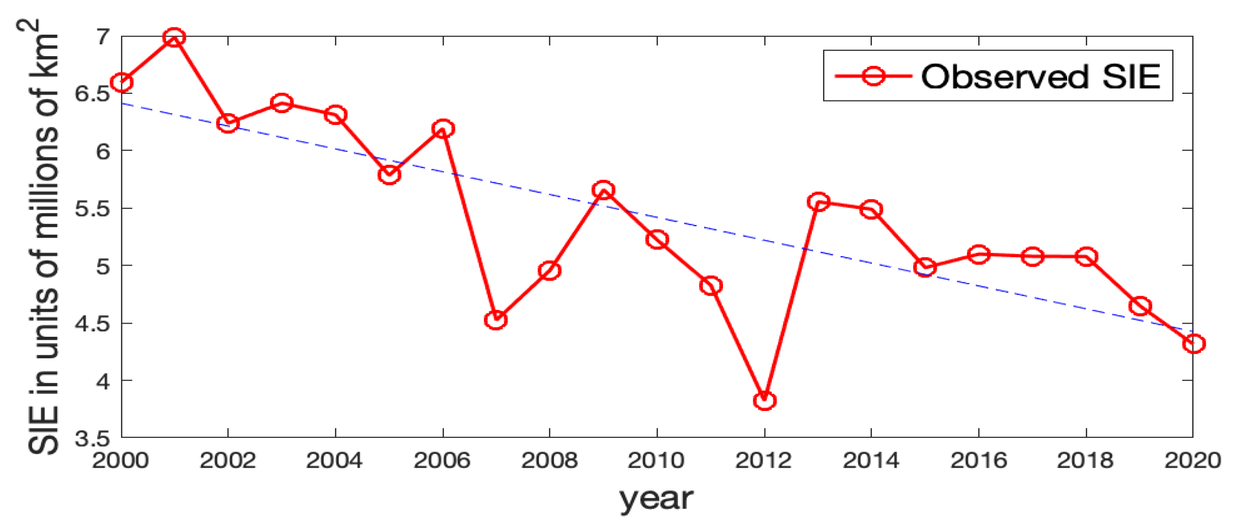
There are many geophysical factors related to the melting of sea ice, such as surface atmospheric temperature [17], the fragility of thinner sea ice [18], the occurrence of the polar anticyclone [19], and reflected solar radiation [20], to name a few, which cause difficulties in characterizing and predicting the presence of Arctic sea ice. Previous analyses have often focused on studying the temporal trend of the obvious summary, sea ice extent (SIE), which is defined as the total area of ice grid cells (grid cells with a sea-ice concentration ≥ 15%) in the Arctic region. Figure 1 shows the observed Arctic SIE in every September over the past two decades, which is derived from the NOAA/NSIDC Climate Data Record of sea ice concentration [21]. By summing up the areas of ice grid cells, we obtained the observed Arctic SIE in each year. An overall declining trend is easily apparent.
The ice/water status in zonal regions is studied here: a zonal band centered at is considered, and from binary ice–water observations on 25 km-resolution remote-sensing grid cells, the proportion of ice grid cells is calculated in each of the ninety longitude–latitude windows that straddle . Then, visualization in the form of boxplots is made from these ninety ice/water proportions. Figure 2 shows a time series of such boxplots five-years apart in latitude bands at N, N, N, …, N. This summary adds a spatial dimension to the time series of SIE shown in Figure 1, illustrating the zonal behavior of sea-ice loss over time. By following the average ice proportions (dots) for each zone, we see that at N, the lowest latitude band, there has been almost no September sea ice since 2000; at N and N, the ice proportions contracted towards zero around 2010; and at N and N, a pre-contraction pattern like that seen earlier at the lower latitudes is emerging.
These exploratory analyses of the observations are useful to detect changing patterns of Arctic sea ice; however, they are based on the aggregated binary data and typically do not come with proper quantification of uncertainty that is obtained by incorporating the spatio-temporal correlations of the data. Statistical models account for the spatio-temporal variability in the underlying ice–water process, as well as the uncertainty inherent in remote-sensing data, and hence they permit valid uncertainty quantification of the resulting summaries. Specifically, the model fitted in this paper allows an estimation of the probability of a grid cell being an ice grid cell in the past and present.
In this paper, we focus on the estimation problem, aiming to use last year’s ice/water statuses at the neighboring locations of a location to estimate its ice/water status in the current year. The main goal is to obtain the estimated ice probability at each spatial location, which may contain more information than a binary outcome. The resulting surface of the estimated ice probabilities is generally smooth and less noisy. Then, various summaries can be obtained based on the estimated ice probabilities to infer the spatio-temporal changes in Arctic sea ice.
Our initial analysis is exploratory, focusing on Arctic binary sea ice data in the month of September, which is when the Arctic SIE typically reaches its minimum in any year and when decline is most likely to occur. Then, a Spatio-Temporal Logistic AutoRegressive (ST-LAR) statistical model is fitted, with spatio-temporally varying coefficients for the remotely sensed binary ice/water data taken in the previous September and defined on 25 km-resolution remote-sensing grid cells. Our model results in smooth estimates at the local level and allows for making inference on zonal and regional features of Arctic sea ice.
The rest of the paper is organized as follows. The related literature is reviewed in Section 2. We describe the data used in our spatio-temporal analysis of Arctic sea ice in Section 3.1. In Section 3.2, we introduce our proposed ST-LAR model, as well as the pseudo-likelihood parameter-estimation procedure used to fit the model. The model-evaluation scores are defined in Section 3.3. In Section 4.1, several models are fitted and compared, resulting in the best-performing model being chosen. Then, in Section 4.2, model-based estimates are presented in terms of summary statistics that describe the spatio-temporal changes of Arctic sea ice. Section 5 contains a resumé of our findings, as well as a brief discussion of future work that might be carried out. Technical details on the proposed model, the regularized estimation procedure, its fast computation, and the detailed model comparison results are contained in the Appendix A, Appendix B and Appendix C.
2. Literature Review
Recently, researchers have used statistical models to capture the spatio-temporal changing patterns of Arctic sea ice. Zhang and Cressie [22,23] proposed a spatio-temporal generalized linear model to model the binary Arctic SIE data, where an Expectation-Maximization (EM) algorithm, e.g., [24], and a fully Bayesian inference were developed, respectively. Horvath et al. [25] proposed a Bayesian logistic regression model to forecast September Arctic SIE, where several atmospheric, oceanic, and sea-ice variables at 1-month to 7-month lead times were used as covariates. Other related works on modeling ice sheet and sea ice belong to the paradigm of applying statistical models to calibrate outcomes from climate models so that the calibrated outputs better match the observed data. For example, Chang et al. [26] proposed a generalized principal component-based method to calibrate the ice sheet of West Antarctica, where principal components were modeled by Gaussian processes. Chang et al. [27] further combined information from both modern and paleo observations to calibrate the ice sheet model. On forecasting Arctic SIE, Director et al. [28] proposed a spatio-temporal statistical model to improve the forecasting of sea ice contours from physical sea ice models; Director et al. [29] further introduced a mixture contour forecasting, which is a weighted average of the recent climatology forecast and the forecast of a statistical model.
Here we adopt another popular route for modeling binary space-time data, a spatio-temporal logistic autoregressive model. The ST-LAR model can be considered as a special case of spatio-temporal autologistic models. Autologistic models, e.g., [30] (Ch.6) have been used extensively for modeling spatial or spatio-temporal binary data, since they have simple forms and directly specify the spatial/spatio-temporal dependence among binary data, e.g., [31,32,33]. Zhu et al. [34] proposed a spatio-temporal autologistic regresson model, which results in a valid spatio-temporal Markov random field for capturing data dependence. Zheng and Zhu [35] and Zhu et al. [36] proposed a Markov chain Monte Carlo method and a Monte Carlo maximum likelihood approach, respectively, to improve the traditional pseudo-likelihood-based estimation for autologistic models. Compared to other spatio-temporal autologistic models, the ST-LAR model does not include current year’s spatially neighboring observations as autoregressors at each time t. We use observations in the previous year as autoregressors, resulting in an ST-LAR model of order one.
Compared to the hierarchical spatio-temporal generalized linear models (GLMs) based on latent Gaussian processes, e.g., [23,37,38], the ST-LAR model directly models the data dependency and is relatively easy and fast to fit using likelihood-based inference. Since the model borrows information from the previous year’s spatially neighboring observations, it encourages estimated ice/water regions to be spatially contiguous. Following recent developments in high-dimensional spatial models (see, e.g., [33,39,40]), the new ST-LAR model we propose has autoregressive coefficients that vary in space and/or time. Spatially varying autoregressive coefficients are capable of capturing the nonhomogeneous autoregressive structure of real data. Our model extends the existing spatio-temporal autoregressive models that have autoregressive coefficients that do not depend on space or time. In addition, it takes into account the neighboring observations’ statuses being 1 (ice) or 0 (water), to allow more modeling flexibility. The proposed ST-LAR model along with regularized estimation of parameters offers a novel and flexible approach for modeling binary spatio-temporal data.
3. Materials and Methods
3.1. Data Description
The datasets upon which our analyses are based are described first, followed by the spatio-temporal statistical models that are fitted to the data. Definitions are then given for the model-evaluation criteria.
Arctic Sea Ice Data. The Arctic sea ice concentration data are produced by the National Oceanic and Atmospheric Administration (NOAA) as part of their National Snow and Ice Data Center’s (NSIDC) Climate Data Record (CDR). The data are obtained from a passive microwave instrument on the Nimbus 7 satellite, as well as from the F8, F11, and F13 satellites of the Defense Meteorological Satellite Program [1,4], which are projected onto grid cells. In this paper, we use Version 4 of the Arctic sea-ice-concentration data, which are available monthly starting from November 1978 [21].
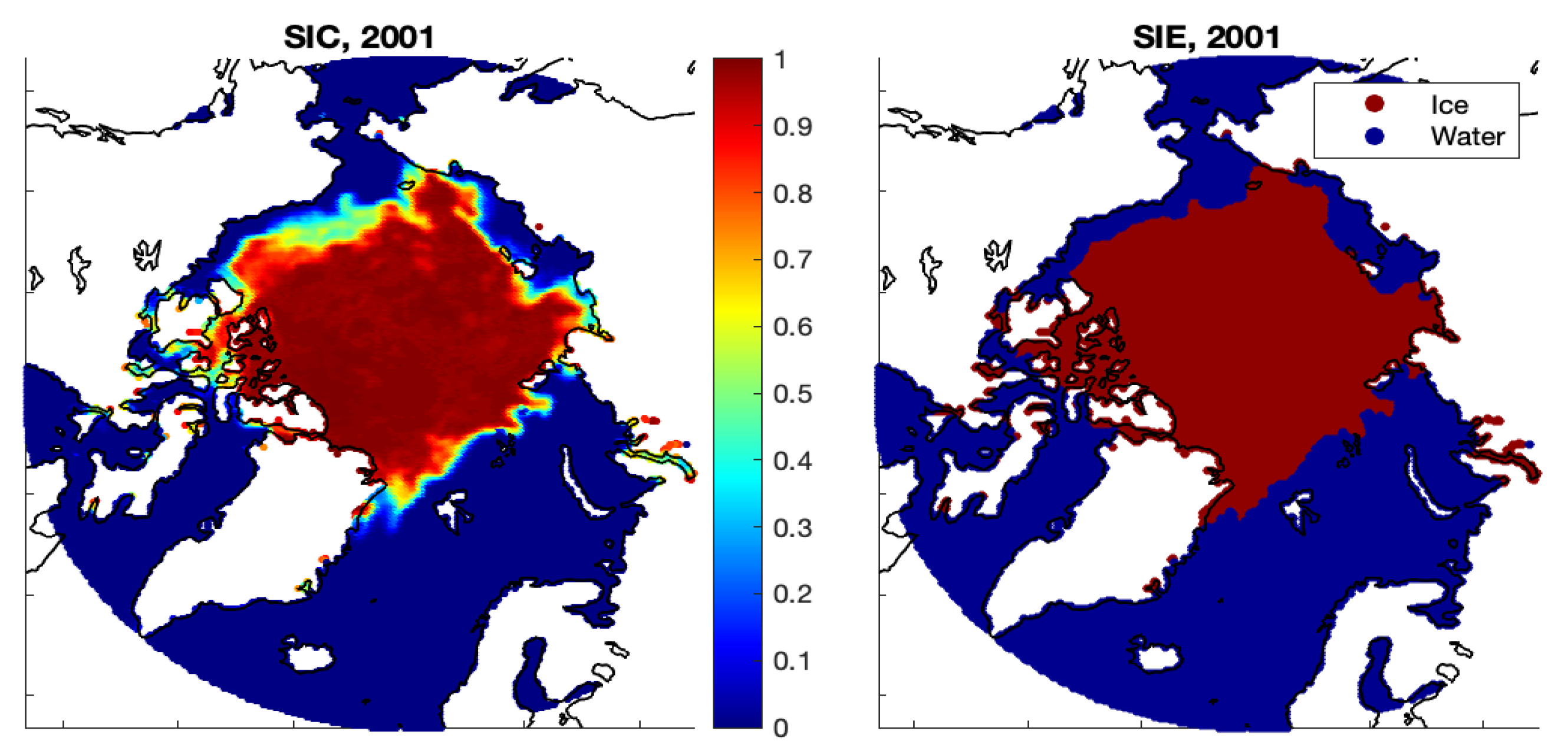
Since the smallest Arctic sea ice cover in a year is typically attained in the month of September [4], we consider the September Arctic sea ice data for the time period from 2000 to 2020, which is a time series at times . The original sea ice concentration data give the fraction of sea ice in each grid cell, taking values in . The sea ice concentration data are from two well-established algorithms, the NASA Team algorithm [41] and the NASA Bootstrap algorithm [42]. To obtain the binary sea ice data, a cut-off value is often used to determine whether a grid cell is water (<15%) or ice (≥15%), e.g., [1,4,43,44]. The original NOAA data are on a grid in a polar stereographic projection but, here, we focus on the grid cells with latitude greater than N, where sea ice is more prevalent. Figure 3, left panel, shows the N cut-off along with the sea ice concentrations; the 25 km-resolution grid cells are small enough not to be distinguishable in the figure. Figure 3, right panel, shows the binary data, where recall that a sea ice concentration ≥ 15% in a grid cell defines it to be an ice grid cell.
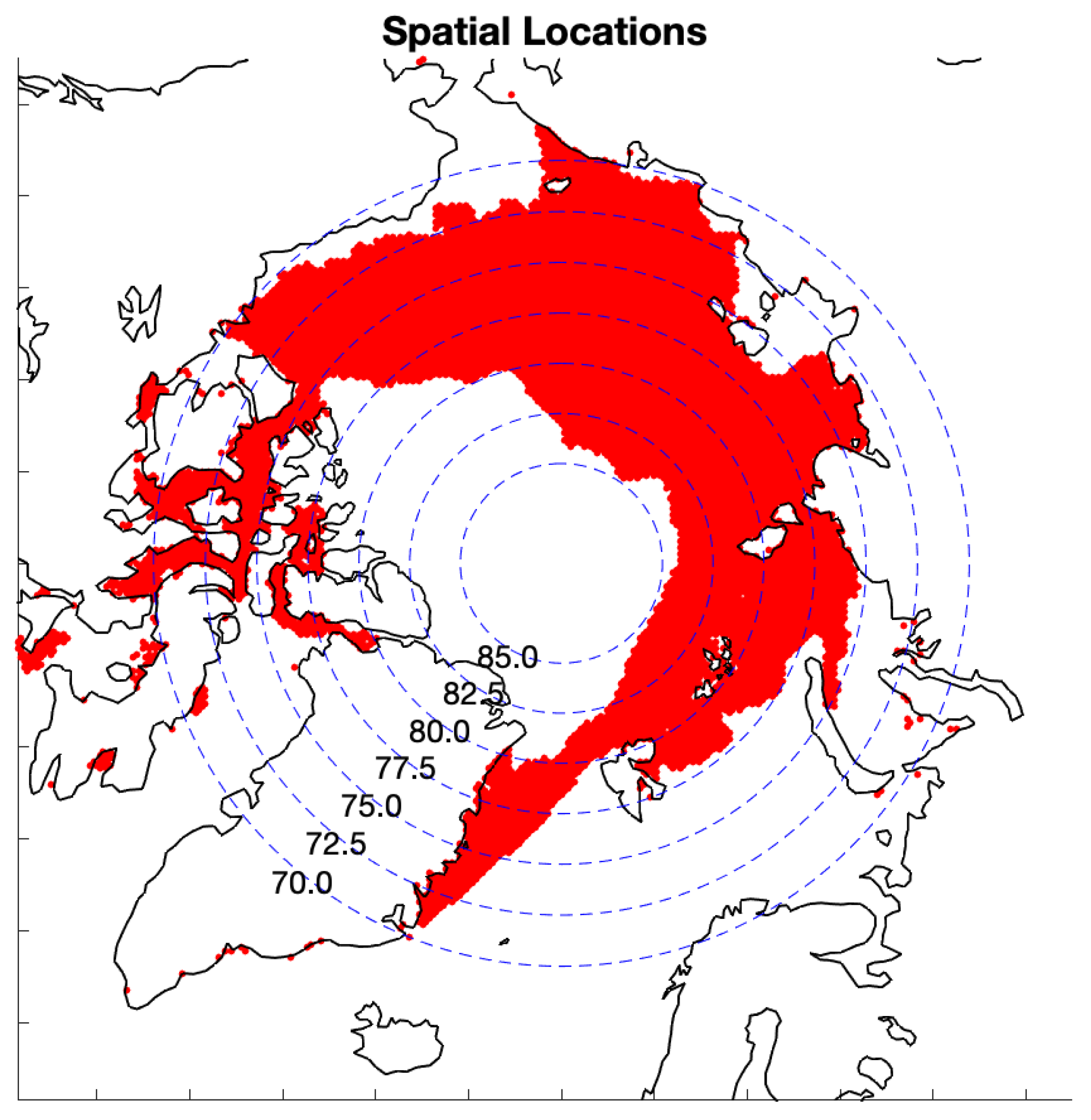
We further select the spatial grid cells that have experienced at least one ice–water or water–ice transition during the entire study period (21 years), leading to the final dataset with 8673 spatial locations (see Figure 4). This spatial domain consists of the union of ice–water boundary regions over two decades.
Reflected Solar Radiation Data. The monthly reflected solar radiation (RSR) data were obtained from NASA’s Clouds and the Earth’s Radiant Energy System (CERES) Energy Balanced and Filled (EBAF) top-of-atmosphere data product [45,46]. Here, we use Edition 4.1 of this data product, which contains monthly shortwave fluxes from March 2000 to January 2021 [47]. The CERES EBAF data product is on a longitude–latitude grid. There are two types of RSR data: one is clear-sky RSR, and the other is all-sky RSR. The clear-sky RSR (CS-RSR) data average the CERES footprints within a region that are cloud-free (defined to be regions where the cloud fraction is no greater than ), which is identified by a cloud-detection algorithm, e.g., [48,49,50]. The all-sky RSR (AS-RSR) data average all the CERES footprints within a region.
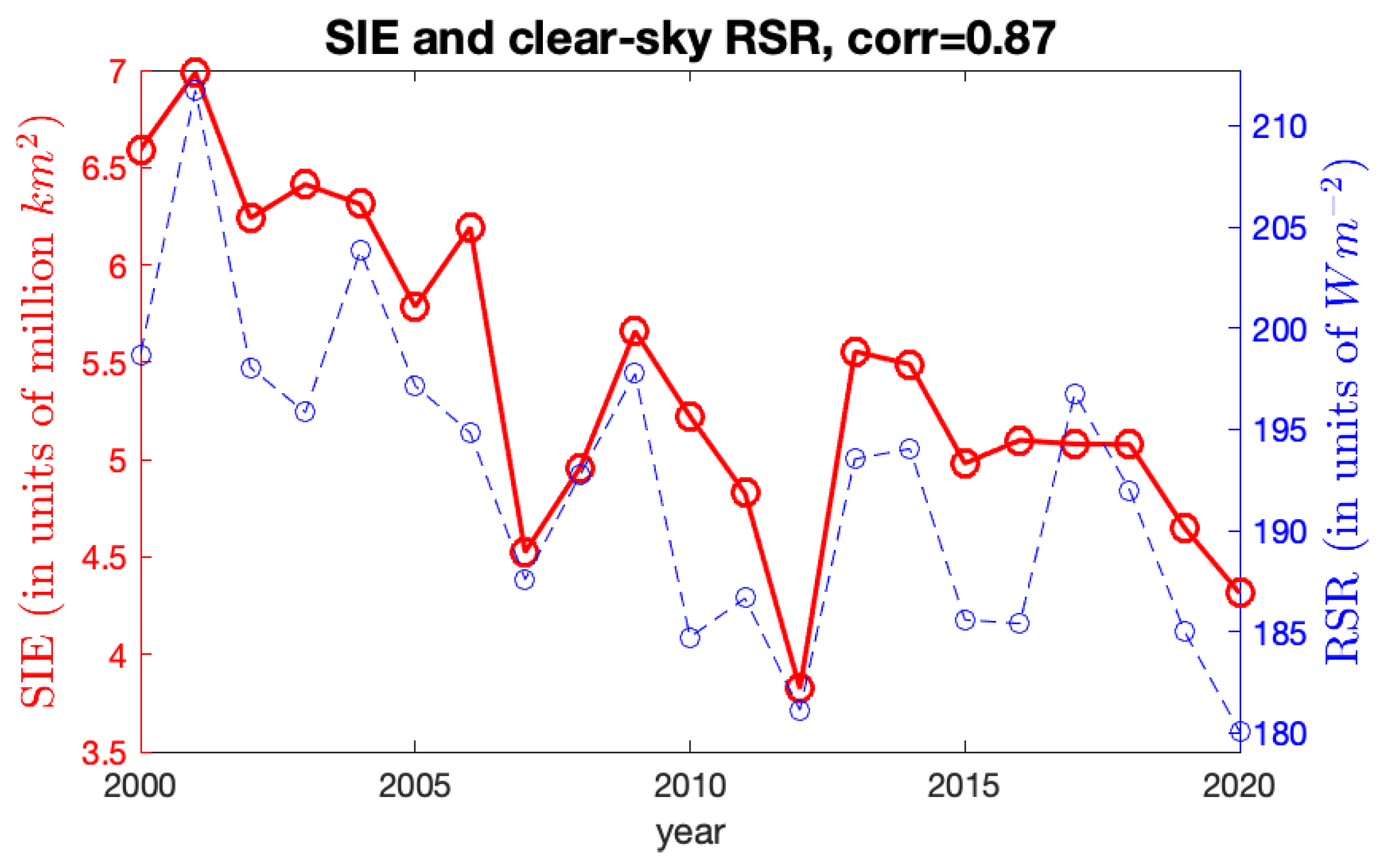
In our analyses, there was very little difference between the two and, henceforth, we show results involving CS-RSR. Spatially averaged CS-RSR, along with the Arctic SIE data for September, are shown as time series in Figure 5. The observed relationship leads us to consider using the June RSR data as an informative covariate in our proposed ST-LAR model.
3.2. Methodology
Notation. We first introduce some mathematical notation. Let denote a spatio-temporal binary datum for a grid cell at spatial location and time point t, where is the two-dimensional Arctic spatial domain and . Recall that is equal to one for an ice grid cell and equal to zero for a water grid cell. Let denote the set of N grid-cell locations where there are data, and we assume does not change over time. The data vector at time t is denoted as , for . We aim to model the probability of being one given all the previous ice/water observations at time , denoted as , where denotes the conditional probability of A given B. We consider a logistic autoregressive model, where the key assumption is that ) depends on covariates at t with regression coefficients , as well as the first-order autoregressive ice/water status of the spatially neighboring observations of at time .
Standard ST-LAR Model. A standard spatio-temporal logistic (first-order) autoregressive model is as follows:
where are the spatially homogeneous regression coefficients associated with the covariate vector , , is the coefficient of the (centered) autoregressor , denotes the set of neighborhood locations of the location , and is the logistic function for . The centered autoregressor directly models the effect of a neighboring water grid cell at (i.e., ) on the presence of an ice grid cell at location and time t, which helps to interpret [32]. In this paper, we focus on the case that , where is the RSR covariate at location and time t.
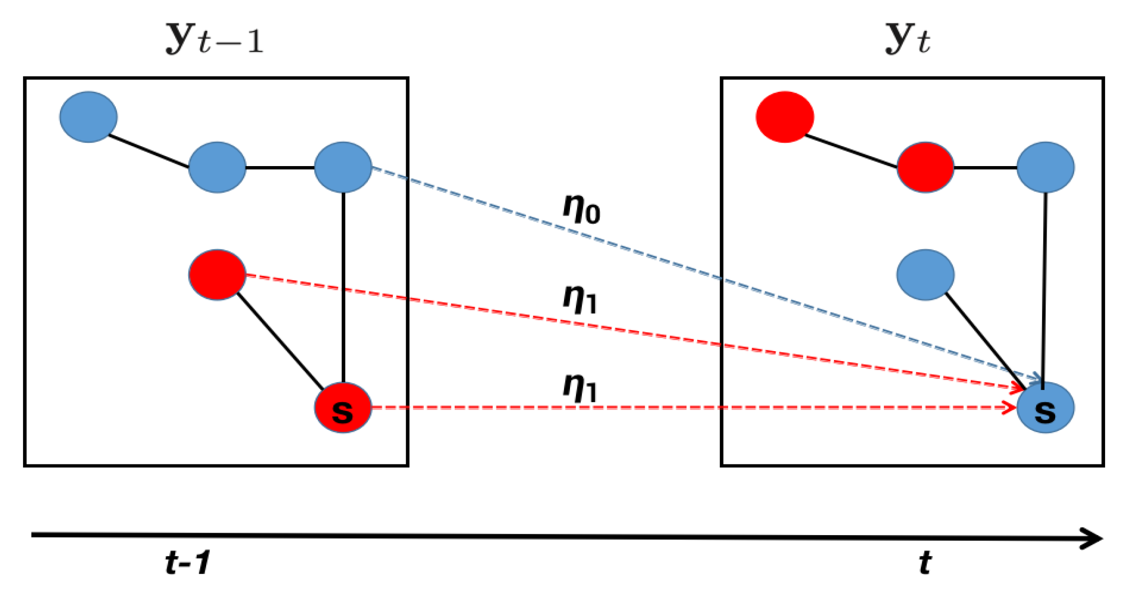
New Proposed ST-LAR Model. The standard ST-LAR model in (1) may be overly simplistic to characterize the complex dependence structure of . To allow more modeling flexibility, we distinguish the effects of spatially neighboring observations at time according to their ice or water status, through using and to denote the corresponding two types of autoregressive coefficients, respectively (see Figure 6 for a conceptual illustration). Moreover, since the effect of covariates and autoregressors may change in space, we allow all the coefficients in the new ST-LAR model to vary with location . In summary, for any location in the observed location set , our proposed model is:
where and denote the index sets of nearby water grid cells and ice grid cells at location and time , respectively. More detailed descriptions of the proposed model are given in Appendix A.
Inference Procedure. Although the proposed logistic autoregressive model with spatially varying coefficients is very flexible, the number of its parameters exceeds the number of observations. To overcome this over-fitting problem, we assume that the spatially varying coefficients are constant within clusters, which can be obtained in an unsupervised manner by imposing a spatially fused LASSO-type penalty [51] on the coefficients in the proposed model. Details on this regularized estimation method are given in Appendix B. We remark that due to the fact that we assume coefficients are clusterwise constant and we impose the fused LASSO penalty to penalize the difference of coefficients at two neighboring spatial locations, the resulting number of distinct coefficients is small relative to the sample size (see Appendix C).
3.3. Model Specification and Model Evaluation Criteria
We consider the ST-LAR model in (2) with different specifications of its coefficients (e.g., the coefficients are constant or spatially varying, and/or the covariate vector does or does not contain RSR). More details on these model specifications are given in Appendix C.
When evaluating the performances of different models, we use the following three criteria: (i) Mean squared error (MSE), which is essentially the Brier score for binary data [52]; (ii) Nash–Sutcliffe model efficiency coefficient (NSE, e.g., [53]); and (iii) correct classification rate (CR). When implementing CR, the probability threshold is used as a cut-off value to transform the estimated ice probabilities to dichotomized estimates taking values 1 (ice) or 0 (water).
Specifically, let denote the fitted ice probabilities; then we have
where , and is the average of the binary data at time t. Note that the NSE score takes values in , with a higher value indicating a greater estimation accuracy. The correct classification rate is
where denotes an indicator function equal to one if A is true and equal to zero otherwise.
4. Analysis of the Arctic Sea Ice Extent Data
In this section, we consider the Arctic SIE data in each month of September from 2000 to 2020, focusing on grid cells in the region greater than N that have experienced at least one ice–water/water–ice transition during the entire study period. The result is a sea ice dataset over 21 years at the 8673 spatial locations illustrated in Figure 4.
4.1. Model Comparison Results
We fitted the ST-LAR model given by (2) to the SIE data in the 2000s and 2010s, with different choices of its coefficients and covariates (see Table A1 in Appendix C). Since the RSR observations are only available from , the data were used as autoregressors to initialize the fitting of the ST-LAR models, and estimates (and ) were obtained from . That is, we fitted the ST-LAR models to the SIE data at spatial locations in the “donut " region, as shown in Figure 4, from which we obtained the corresponding estimated ice probabilities and model evaluation scores from to .
From the model comparison results given in Appendix C, the best model takes the following form:
where and are the index sets consisting of the neighboring water grid cells and ice grid cells for location at time , respectively. That is, the best model has spatially varying coefficients for the intercept and the autoregressive coefficients, and it does not have any covariates.
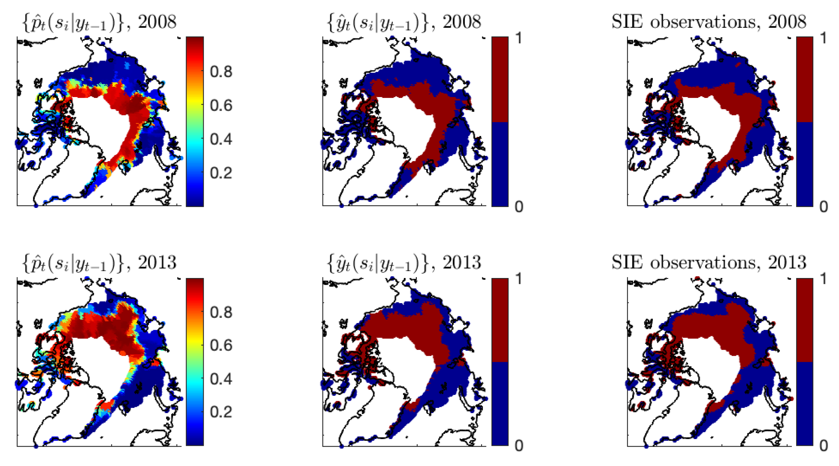
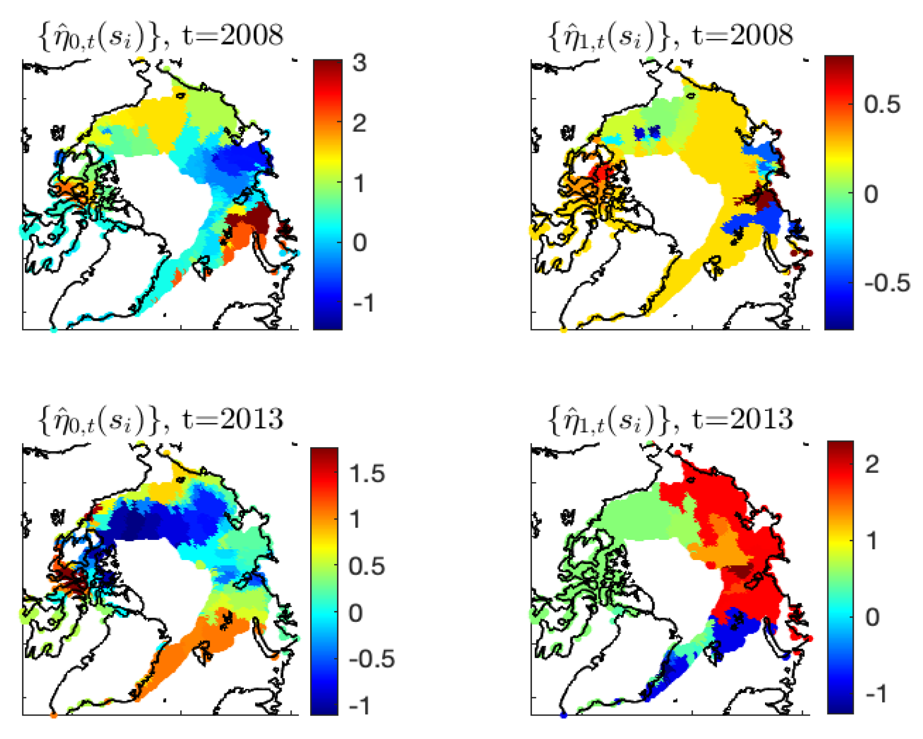
Our numerical results in Appendix C show that the standard ST-LAR model with spatially constant coefficients but without the RSR covariate cannot capture the spatial behaviors of the observed ice–water/water–ice transitions, resulting in low model evaluation scores (see Table A2). When allowing the -coefficients to vary over the spatial domain , the estimates match the observed ice/water status very well (see Figure A2), and the inferred dichotomized ice/water estimates using the cut-off value result in high correct classification rate (CR) scores. Furthermore, allowing the intercept to also vary in space slightly improves the CR scores, where significant improvements occur in years and . Figure 7 shows the estimation results of the model fitted according to (3), compared to the SIE observations, for and 2013. Clearly, match the spatial patterns of the binary Arctic SIE data for those years very well. The excellent performance of our proposed model (3) can be attributed to its spatially varying coefficients, whose values can adapt to the observed ice–water/water–ice transitions in regions that lose or gain substantial sea ice from to t (see Figure 8).
We also considered the model given by (2) with spatially constant autoregressive coefficients and covariate given by the June reflected solar radiation (RSR) in the same year, but the model evaluation scores were not competitive (Table A3 in Appendix C). Furthermore, when using spatially varying autoregressive coefficients and the RSR covariate, it did not improve on average the model evaluation scores of the model without the RSR covariate.
Henceforth, we focus on the estimates from the model given by (3) and propose several summaries of them to reflect the spatio-temporal changes in Arctic sea ice over the two decades from 2000 to 2020. These summaries are intended to visually capture the decline in Arctic sea ice in the 2000s and the 2010s.
4.2. Summaries Based on the Model Given by (3)
We first consider the Arctic SIE, which is defined as the sum of areas of all ice grid cells in the Arctic region. By setting using the estimated ice probability, , from the best model, we obtain dichotomized ice/water estimates at spatial locations that experienced at least one ice–water transition in the past two decades (i.e., 8673 locations in the “donut” region). For the remaining locations that were always ice or always water during these two decades, we simply let
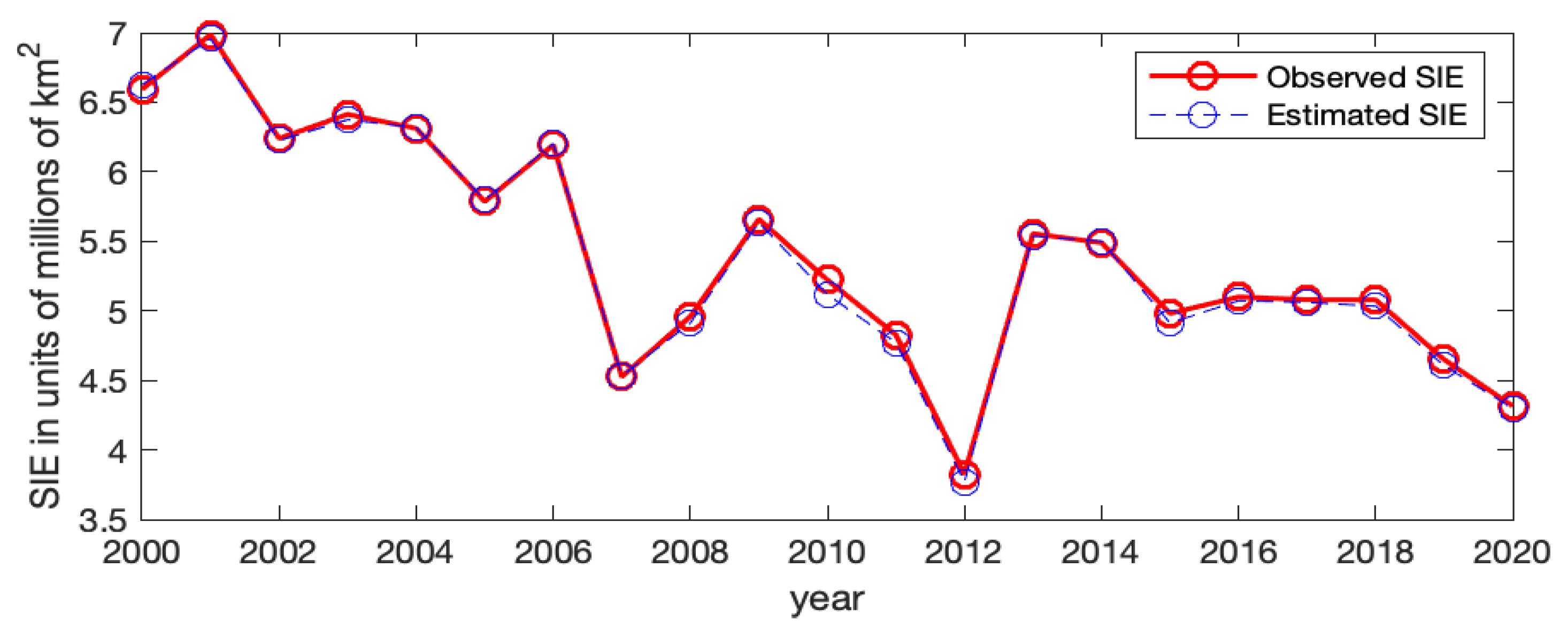
Then, by summing up the areas of the estimated ice grid cells, we obtain the estimated Arctic SIE. From Figure 9, we can see that the time series of estimated SIEs agrees with the time series of observed SIEs very well.
Next, similarly to the exploratory analysis shown in Figure 2, we can describe the zonal changes in sea ice at different latitude bands by summarizing the estimates , obtained from (3) and (4). Then, for a latitude band centered at with half-bandwidth equal to , we can summarize the estimates within this latitude band over .
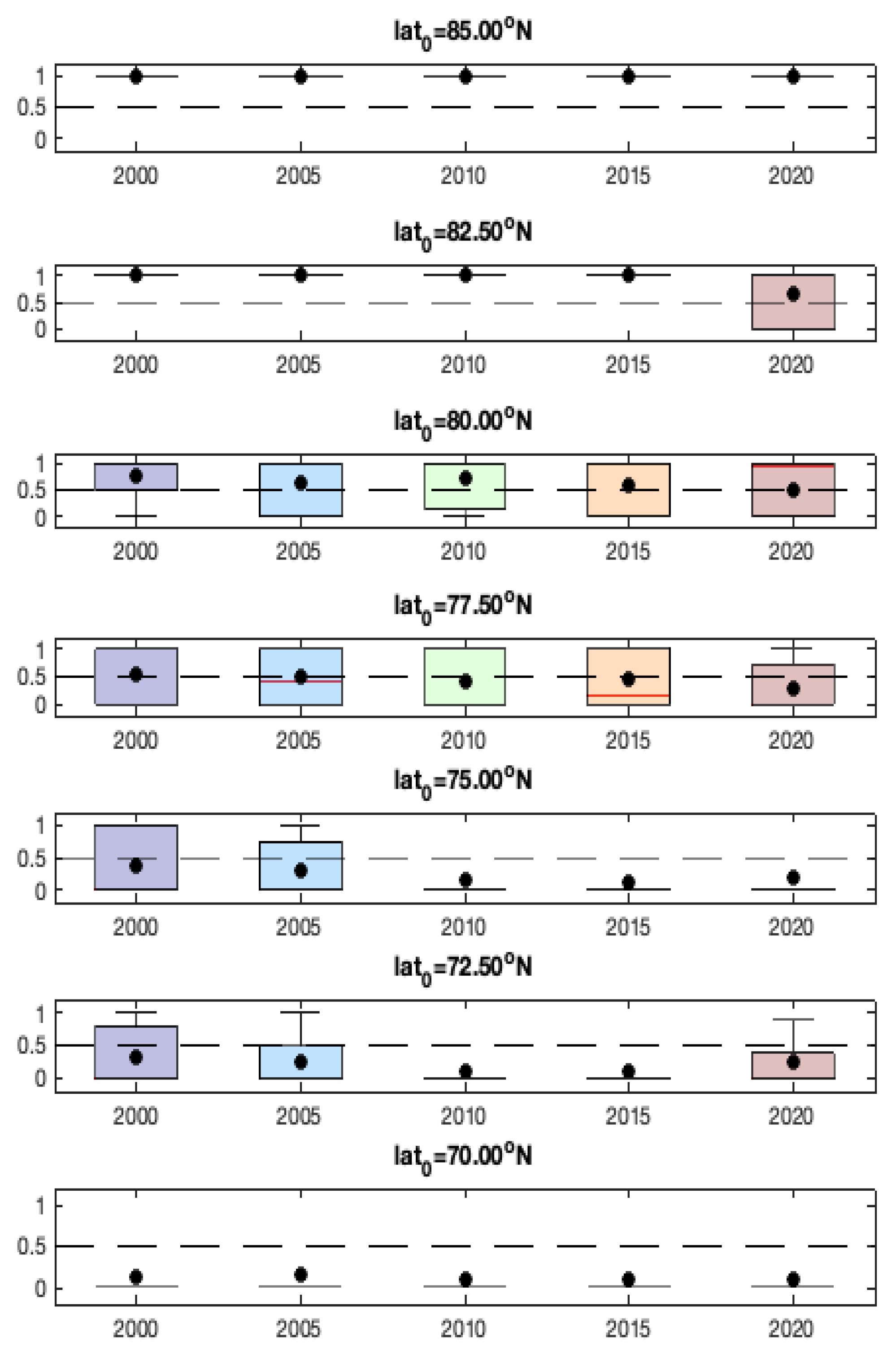
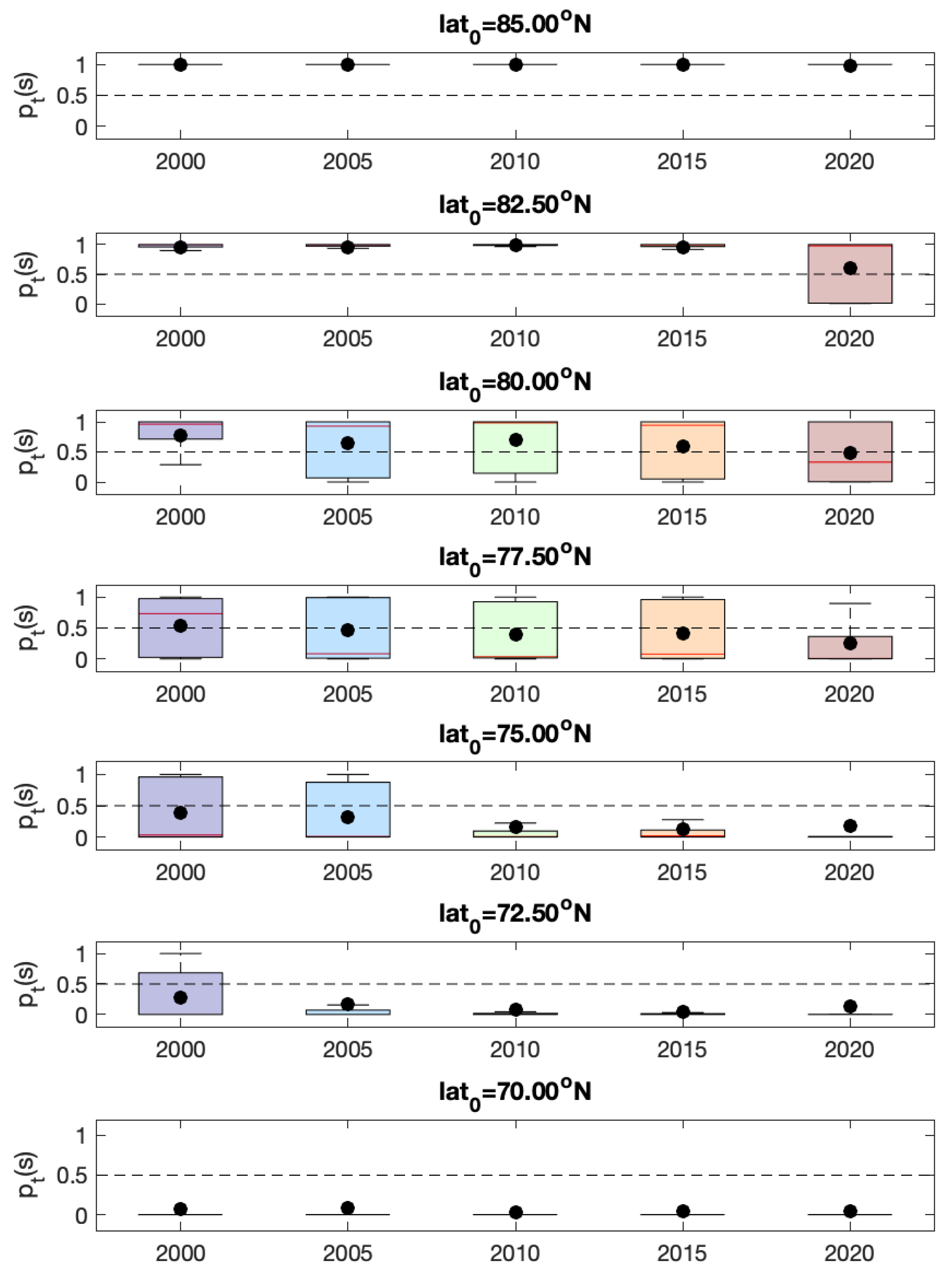
Figure 10 shows time series of such boxplots for latitude bands N, N, N, N, N, N, and N at five-year intervals from 2000 to 2020. For each latitude band with bandwidth , the estimates with latitudes in are summarized; we chose , resulting in a latitude bandwidth of . Since these boxplots are made at a finer resolution than the exploratory results in Figure 2, the changes in sea ice both in level and variability are more apparent. We can see that for the mid-high latitude bands , there is a clear deceasing temporal trend of over the past two decades. Even for the higher latitude band , the estimated ice probabilities have large variations at compared to those concentrated near one with a small interquartile range in the previous years. Critically for , once the third quartile of drops below , the sea ice almost disappears in later years and never rebounds afterwards. This behavior may reflect the future trend of the ice probabilities for the higher latitude bands such as (and even ), under climate change.
5. Discussion and Conclusions
In summary, we consider ST-LAR models with spatially varying coefficients to characterize the changes in sea ice in the Arctic, where the probability of a grid cell at location and time t being ice (i.e., ) depends on the observations in at the neighboring grid cells of . Compared to standard ST-LAR models, we allow the autoregressive coefficients (-parameters) to vary in space and time to capture local spatial variations in the binary Arctic sea ice data. The effects of autoregressors are distinguished according to their ice/water statuses to allow more modeling flexibility. To reduce the number of spatially varying parameters, we employed a regularized estimation approach using spatially fused LASSO penalties to yield clusterwise constant parameters. The proposed model, along with regularized estimation, offers a novel and flexible approach for modeling binary spatio-temporal data. The spatially varying autoregressive coefficients can adapt to the nonhomogeneous autoregressive structure of the Arctic sea ice data, thus leading to superior fitting results. Our results show that with spatially varying autoregressive coefficients, the estimated ice probabilities can capture the spatial patterns of observed ice–water/water–ice transitions very well.
We found that with spatially varying autoregressive coefficients, further adding the RSR covariate to the ST-LAR models did not significantly improve the estimation results. The best model form has spatially varying autoregressive coefficients and a spatially varying intercept, as given in (3). This model results in correct classification rates generally above for each year. Based on the estimated ice probabilities of the best model, we computed several summary statistics to describe the spatio-temporal changes in Arctic sea ice. For the time series of Arctic SIE, the estimated SIEs match the observed ones very well and show a clear declining temporal trend over the past two decades. Then, the estimated ice probabilities were summarized zonally in selected latitude bands through a time series of boxplots for each latitude band over different years. We observed that for the mid-high latitude bands, there is a clear declining trend of the estimated ice probabilities over the past two decades. For latitude bands at and , the sea ice almost disappeared after 2010 and did not rebound afterwards. A similar zonal contraction towards zero may now be underway for the higher latitudes and , since the estimated ice probabilities already show decreasing levels and/or increasing variabilities from 2000 to 2020.
By assuming are conditionally independent given and model parameters at each time t, the proposed ST-LAR model leads to a valid joint distribution for . Hence, the parametric bootstrap approach [54] can be applied to obtain the standard errors of parameter estimates and the estimated ice probabilities (see Appendix C). While it can be time-consuming to run the model on multiple bootstrap samples, importantly, it results in valid statistical inferences.
In this paper, we focus on obtaining the estimated ice probabilities in the Arctic region. Since the spatial-specific coefficients in the proposed ST-LAR model are estimated using data at time t, our model cannot be readily used to predict the ice/water status in future years. To enable forecasting, we need to assume that the autoregressive relationship does not change in a short time period. The choice of a suitable time window in which the autoregressive structure approximately stays the same will need further investigation. We leave investigating the forecasting aspect of ST-LAR models for future research. In addition, the Arctic SIE data at targeted months in the same year can also be considered for constructing the autoregressors in an ST-LAR model, e.g., [25,55].
Author Contributions
B.Z., F.L. and H.S. developed the method; N.C. and B.Z. designed the summary statistics and visualizations; B.Z. and F.L. obtained the numerical results; B.Z. prepared the original manuscript, which was reviewed and edited by N.C. and H.S. All authors have read and agreed to the published version of the manuscript.
Funding
Zhang’s research was supported by the National Science Foundation China (11901316), and the Fundamental Research Funds for the Central Universities, Nankai University (63201156), China. Li’s research was supported by the National Science Foundation China (41906011). Sang’s research was partially supported by the U.S. National Science Foundation, grant number DMS-1854655. Cressie’s research was supported by Australian Research Council Discovery Project DP190100180.
Institutional Review Board Statement
Not applicable.
Informed Consent Statement
Not applicable.
Data Availability Statement
Not applicable.
Acknowledgments
We are grateful to the reviewers and editor of earlier versions of the paper for their suggested improvements. We thank National Oceanic and Atmospheric Administration (NOAA) and National Snow and Ice Data Center’s (NSIDC) for sharing the Arctic sea ice concentration data. We thank NASA’s Clouds and the Earth’s Radiant Energy System (CERES) for sharing the Energy Balanced and Filled (EBAF) top-of-atmosphere data product.
Conflicts of Interest
The authors declare no conflict of interest.
Appendix A. Modeling Details
For the most general ST-LAR model in (2), is the (normalized) p-dimensional covariate vector at location and time t, is the vector of regression coefficients, denotes the index set of water grid cells at time , and denotes the index set of ice grid cells at time .
Since the spatially neighboring observations of are more likely to affect its own status (e.g., intuitively, a spatial grid cell surrounded by ice/water grid cells in the last year is more likely to be an ice/water grid cell in the current year t, we further assume that only depends on its spatial neighbors at . When defining the spatial neighborhood of a location , we may use the nearest neighbors of for some positive integer m, mimicking the m-th order spatial autoregression model on a lattice. In this paper, we chose to specify 8 neighbors for each location. Let denote the pre-specified index set of the spatially neighboring locations of ; now for , the conditioning index sets for are and . By using these index sets, the model in (2) implies that are conditionally independent given their spatially neighboring observations in .
Since the model in (2) assumes spatially and temporally varying coefficients, it involves parameters, whose number exceeds the sample size . In practice, for spatial location , the spatio-temporal dependencies in and its spatial neighbors often behave similarly, resulting in spatial patterns for the -coefficients and -coefficients in (2). Thus, it is often reasonable to assume that these coefficients are clusterwise constant, thus reducing the total number of parameters. Following the regularized estimation procedure proposed by Li and Sang [40], at each time point t, we shall penalize the differences of , , and between and its spatial neighbors to obtain spatially cluster-wise constant coefficients. This is achieved by imposing a fused LASSO-type penalty [51] on the log-likelihood function when estimating model parameters, which will be discussed in Appendix B.
Appendix B. Regularized Estimation Method
In this section, we describe a general regularized pseudo-likelihood parameter-estimation procedure for our proposed ST-LAR model in (2), which applies to all the model specifications in this paper.
To ease notation, let for short, let denote the conditional probability of being one given , and let denote the vector stacking the regressors , , and in (2) corresponding to , for and . Let denote the parameter vector at location and time t; using the notations given above, we can rewrite in (2) as .
Let denote the set of all parameters associated with the model (2). In the absence of instantaneous spatial dependence, which leaves conditionally independent given , the (pseudo) log-likelihood, e.g., [56] over is given by the equally-weighted sum of the log conditional densities of :
where .
We assume that the location-specific -coefficients and -coefficients have a clustering pattern in space, and a fused LASSO-type penalty [51] is imposed on the log-likelihood given by (A1). Following the work by Li and Sang [40], we first obtain a partial order of the observed spatial locations using a tree graph to facilitate computations while preserving spatial information. Then, homogeneity constraints are imposed on each pair of coefficients at two adjacent locations, where the adjacencies of locations are defined by the edges of the tree graph. We shall remark here that the graph used to construct the fused LASSO penalty can be different from the graph used to define the neighboring autoregressors in (2).
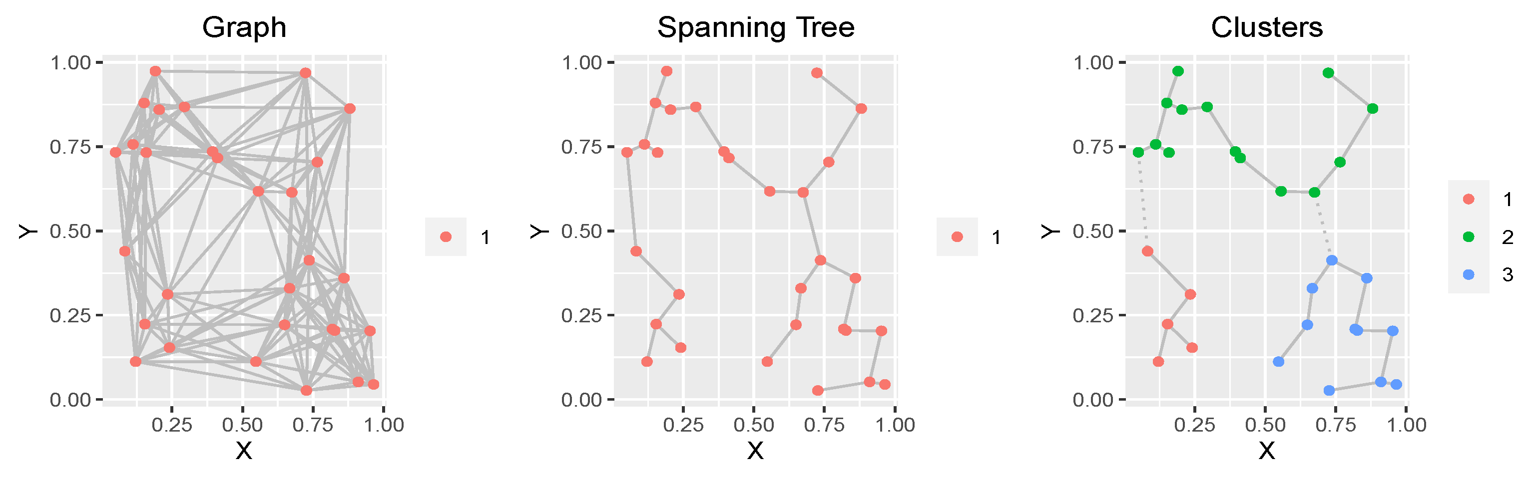
Specifically, we first define location neighborhoods using a connected undirected graph , with the M spatial locations as its nodes. In practice, we can either use a Delaunay triangulation [57] or a k-nearest neighbors approach to construct such a graph . Then, we assign the edges of with Euclidean distances of the nodes as the edge weights. For edges with the same weights, we break the tie by adding a very small random perturbation to each edge weight. A compact representation of the neighboring structure of those spatial locations is given by a spanning tree of , which is a connected subgraph of with the same nodes but without any cycles. Then, the unique minimum spanning tree (MST) is obtained by minimizing the sum of edge weights among all the spanning trees of . For example, the left panel of Figure A1 shows a connected graph with 30 nodes, which is constructed by connecting each node with its 10 nearest-neighboring locations. The corresponding MST of is shown in the middle panel of Figure A1. Then, by deleting edges from the MST, we can naturally define r clusters as the r sub-trees of the MST (see the right panel of Figure A1 for the clusters after removing the edges with the two largest weights).
Figure A1.
Left panel: A connected graph of 30 nodes, where each node is connected with its 10 nearest (according to Euclidean distance) neighbors, and edge weights are equal to the Euclidean distances between the nodes. Middle panel: The minimum spanning tree of . Right panel: The three induced clusters by removing two edges of the spanning tree (the two dotted lines).

Let denote an MST of , where is the vertex set of M nodes and is the edge set. We minimize the following objective function:
where denotes an edge in connecting locations and , and
Thus, at each time t, zero values of , , and correspond to the edges connecting internal points of a cluster for the -coefficients and the -coefficients, respectively, while the nonzero values of these correspond to the edges connecting two boundary points across two clusters. For example, if are only different at the adjacent locations connected by the dotted lines in the right panel of Figure A1, we can obtain three clusters for the k-th regression coefficient by deleting these two edges.
Suppose an edge connects two locations and for , where is the number of edges in the MST, and let denote the M-dimensional vector with only two nonzero entries: 1 at the i-th index and at the j-th. Then, , where , and and are similarly defined.
Let denote the contrast matrix; then, the penalized negative log-likelihood function can be written as
where denotes the norm of the vector .
Following [40], by letting and , we can re-parameterize the model parameters as , , and , for . Let denote the vector of all the re-parameterized model parameters; since is invertible by construction, minimizing the penalized negative log-likelihood in (A3) is equivalent to minimizing
where and are the column vectors containing the first entries of and , respectively. Minimizing the objective function in (A4) is a standard LASSO problem whose computation is efficient. The best tuning parameter in (A4) is selected from a number of proposed values according to a model selection criterion, such as the Akaike information criterion (AIC, e.g., [58]) or the Bayesian information criterion (BIC, e.g., [59]). In our application to Arctic sea ice, we chose BIC to select .
Appendix C. Detailed Model Comparison Results
To model the September Arctic sea ice data, consider the ST-LAR model in (2) and its special cases as summarized in the following Table A1. The Model-1 class only uses an intercept term for modeling the mean of , which has three sub-cases: (a) the intercept is constant and the -coefficients are time-varying; (b) the intercept is time-varying and the -coefficients vary in space and time; and (c) both the intercept term and the -coefficients vary in space and time. Since for Model-1a the constant is used instead of , the design matrix of , , and is of full rank. The Model-2 class incorporates June’s reflected solar radiation (RSR) as a covariate (denoted by ) in the ST-LAR model, which includes four sub-cases depending on whether the coefficients vary purely in time or vary in both space and time. The two classes and their sub-cases are specified in Table A1.

Table A1.
The ST-LAR models for fitting the September Arctic SIE data. The mean of the latent is either modeled by an intercept term or by using the RSR as a covariate.
Table A1.
The ST-LAR models for fitting the September Arctic SIE data. The mean of the latent is either modeled by an intercept term or by using the RSR as a covariate.
| Model-1a | |
| Model-1b | |
| Model-1c | |
| Model-2a | |
| Model-2b | |
| Model-2c | |
| Model-2d |
Model evaluation results of different ST-LAR models were obtained at locations with at least one observed ice–water/water–ice transition in the last two decades. When implementing the regularized estimation given in Appendix B, we tried different values of ranging from to 10 and selected the best one using the BIC criterion. The selected values are different at different years, and the median value is about .
Initialization for Estimation. Our proposed ST-LAR model given by (2) requires (centered) past observations at time as autoregressors to model the ice probability at time t. At the initial year , since the means of (i.e., ) are not available, we set -coefficients in model (2) to zero and only use -coefficients to fit the binary observations at . After we obtain the estimates , we can fully employ the ST-LAR models in Table A1 and obtain the estimated ice probabilities in a progressive manner from onwards.
Results of the Model-1 Class. We first considered Model-1a, which uses a constant intercept for modeling the mean of and assumes only time-varying -coefficients. We used all the data to estimate the intercept through a classical logistic regression, assuming no space-time dependence among the observations. Then, by fixing at its estimate, a simple logistic regression was used to estimate and at each time point.
The corresponding model fitting results of Model-1a are given in the left columns of Table A2. We observe that the MSE values are generally large compared to those in the middle and right columns, and the correct classification rates using the cut-off value are generally below . This indicates that only using the constant -coefficients at each time point is not flexible enough to capture the spatial behaviors of ice–water/water–ice transitions. Then, we considered a more flexible model allowing the -parameters to vary in space and time (Model-1b), and it can be seen that the fitting results are greatly improved (see the middle columns of Table A2): The averaged MSE has reduced from Model-1a by a factor between 3 and 4, and the averaged correct classification rate is about compared to for Model-1a, indicating that the fitted ice probabilities can capture the observations very well. When further allowing the intercept to vary in space and time (Model-1c), the resulting averaged model evaluation scores are only slightly better than those of Model-1b. We observe that improvements in prediction accuracy for Model-1c occur for years 2004, 2008, 2013, 2016, 2017, and 2020. The performances of Model-1b and Model-1c are generally comparable, but Model-1b yields relatively lower correct classification rates at () and ().
Table A2.
Model evaluation scores: The mean squared errors (MSEs), Nash–Sutcliffe model efficiency coefficients (NSEs), and the correct classification rates (CRs) for the Model-1 class based on their estimates at . The last row gives the time-averaged model evaluation scores.
Table A2.
Model evaluation scores: The mean squared errors (MSEs), Nash–Sutcliffe model efficiency coefficients (NSEs), and the correct classification rates (CRs) for the Model-1 class based on their estimates at . The last row gives the time-averaged model evaluation scores.
| Model-1a | Model-1b | Model-1c | |||||||
|---|---|---|---|---|---|---|---|---|---|
| Year | MSE | NSE | CR | MSE | NSE | CR | MSE | NSE | CR |
| 2001 | |||||||||
| 2002 | |||||||||
| 2003 | |||||||||
| 2004 | |||||||||
| 2005 | |||||||||
| 2006 | |||||||||
| 2007 | |||||||||
| 2008 | |||||||||
| 2009 | |||||||||
| 2010 | |||||||||
| 2011 | |||||||||
| 2012 | |||||||||
| 2013 | |||||||||
| 2014 | |||||||||
| 2015 | |||||||||
| 2016 | |||||||||
| 2017 | |||||||||
| 2018 | |||||||||
| 2019 | |||||||||
| 2020 | |||||||||
| Average | |||||||||
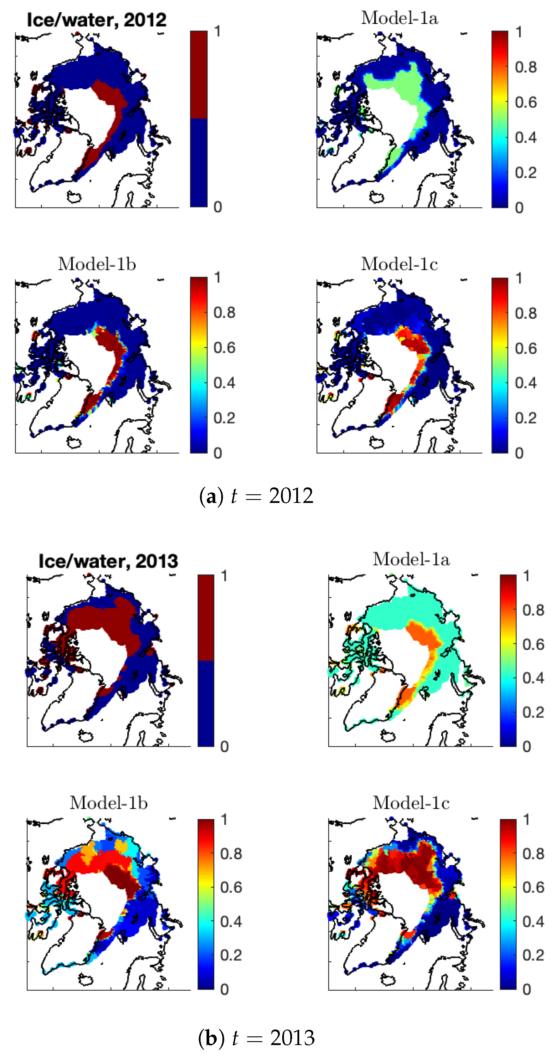
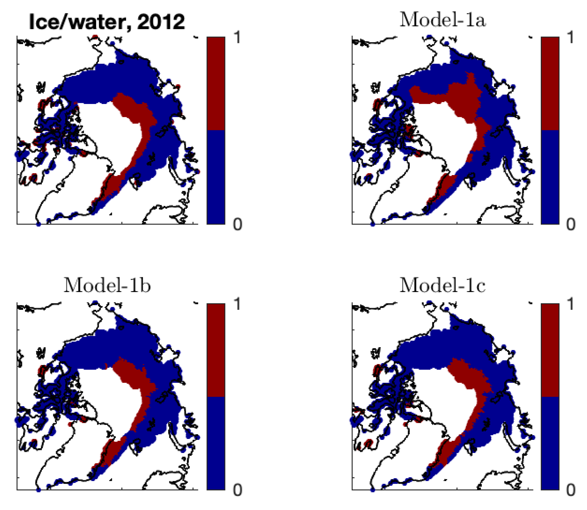
Figure A2 shows the estimates of made by different models versus the observed SIE data at years . It is clear that the simple autoregressive model with parameters cannot capture the spatial patterns of the ice/water statuses at time t; in fact, its estimated probabilities behave similarly to the immediate past observations at . In contrast, by allowing the -coefficients to vary in space and time, Model-1b can capture the main spatial patterns of the observed ice/water statuses, resulting in the estimates of behaving very similarly to the observations. We can see that in 2012, the estimates of by Model-1b are almost dichotomized, with small variations in the ice–water boundary regions. In the following year, 2013, Model-1b does not have the flexibility to capture the dramatic ice–water transitions, resulting in an estimated probability surface of substantial variability. Here, the fitted probabilities of Model-1c, which further allows the intercept to vary in space as well as time, behave more similarly to the observations.
Figure A2.
For each of (a) and (b) , shown are the observed ice/water statuses (upper-left panel) and the estimated ice probabilities by Model-1a (upper-right panel), Model-1b (lower-left panel), and Model-1c (lower-right panel).
Figure A2.
For each of (a) and (b) , shown are the observed ice/water statuses (upper-left panel) and the estimated ice probabilities by Model-1a (upper-right panel), Model-1b (lower-left panel), and Model-1c (lower-right panel).

In addition, we obtain the binary estimates by applying the cut-off value of to dichotomize the sea-ice concentration estimates . Both Model-1b and Model-1c lead to estimated ice/water statuses that are very similar to the observed statuses (see Figure A3).
Figure A3.
The observed ice/water status and the estimated ice/water status (by Model-1a, Model-1b, and Model-1c) at .
Figure A3.
The observed ice/water status and the estimated ice/water status (by Model-1a, Model-1b, and Model-1c) at .

Results of the Model-2 Class. Zhan and Davies [20] used the June RSR data to estimate the September Arctic sea ice with good success. This motivates us to include the June RSR as a covariate in our new model given by (2) to see whether the model evaluation scores can be improved further. At each time t, we standardized the RSR data by subtracting the sample means over space and dividing by the corresponding standard deviations. The CERES EBAF data product is on a longitude–latitude grid, whose resolution is different from the 25 km resolution of the remotely sensed Arctic sea-ice data. When modeling , we used the June RSR value at the location nearest to as its RSR covariate.
The results of the Model-2 class are given in Table A3, where the clear-sky RSR (CS-RSR) was used as a covariate when modeling . For the model (2) with spatially constant coefficients , after incorporating the CS-RSR as a covariate (Model-2a), the correct classification rates have improved somewhat, with an averaged correct classification rate of , compared to with Model-1a. Especially for year , from Table A2, Model-1a has a very low correct classification rate of and a very small NSE value of . By borrowing information from the CS-RSR in 2013, Table A3 shows that Model-2a achieves an improved correct classification rate of and a much bigger NSE score. Changing the CS-RSR covariate to the AS-RSR covariate made very little difference in terms of the three model evaluation scores.
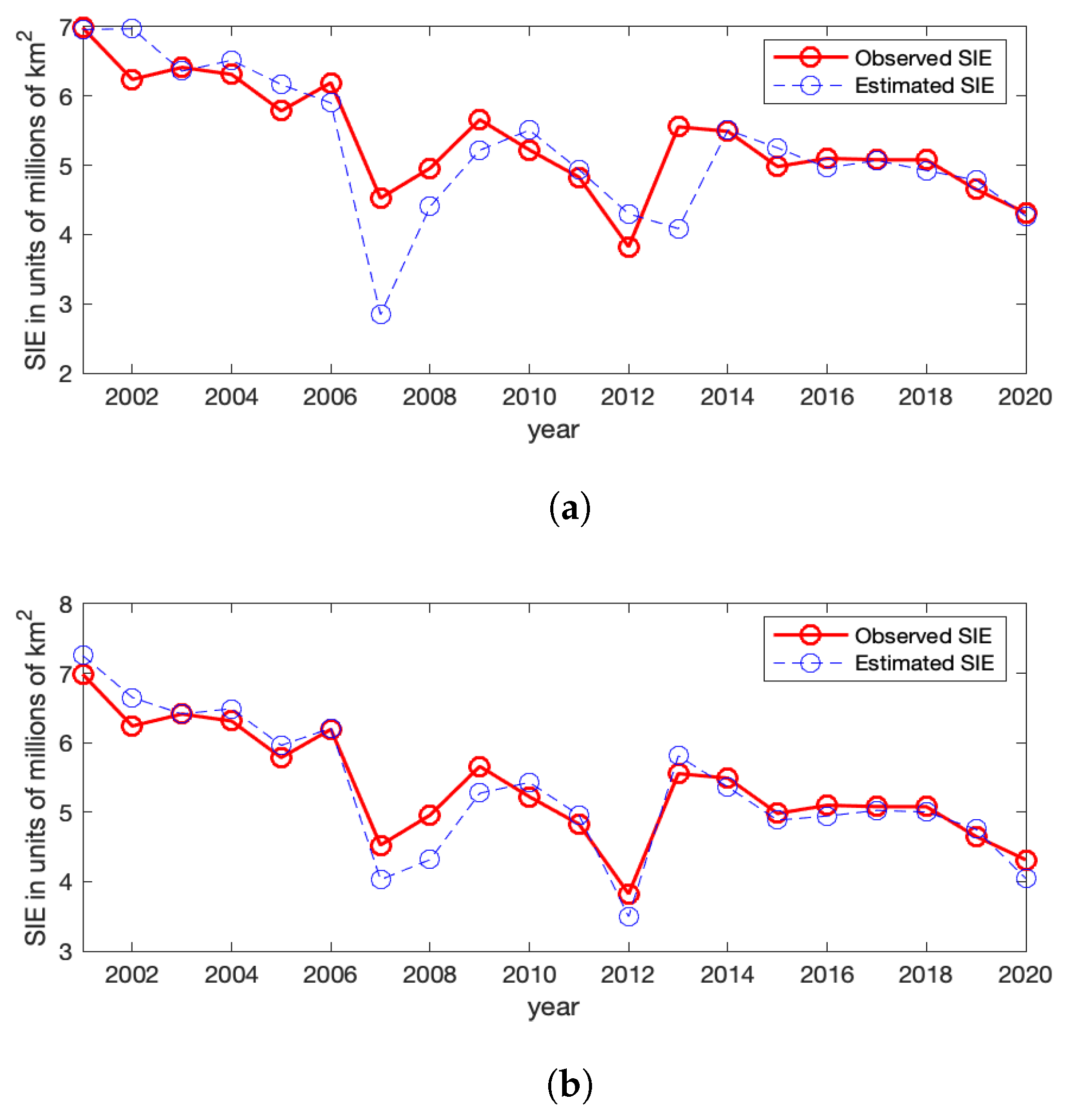
Figure A4 shows the observed Arctic SIE values and the estimated ones for Model-1a and Model-2a without and with CS-RSR, respectively. For Model-1a, which does not involve the RSR covariate, its ice/water statuses have large discrepancies with the observed values at a few years, and the general temporal trend of the SIEs cannot be captured; for example, the fitted Arctic SIEs are much smaller than the observed values at and 2013. In contrast, when incorporating the June RSR information into the model (Model-2a), the estimated ice/water statuses are much closer to the observed values. Hence, the June RSR variable seems to be helpful for modeling Arctic sea ice.
Table A3.
The MSEs, NSEs, and CRs for the Model-2 class with clear-sky RSR (CS-RSR) as a covariate. The last row gives the time-averaged model evaluation scores.
Table A3.
The MSEs, NSEs, and CRs for the Model-2 class with clear-sky RSR (CS-RSR) as a covariate. The last row gives the time-averaged model evaluation scores.
| Model-2a | Model-2b | Model-2c | Model-2d | |||||||||
|---|---|---|---|---|---|---|---|---|---|---|---|---|
| Year | MSE | NSE | CR | MSE | NSE | CR | MSE | NSE | CR | MSE | NSE | CR |
| 2001 | ||||||||||||
| 2002 | ||||||||||||
| 2003 | ||||||||||||
| 2004 | ||||||||||||
| 2005 | ||||||||||||
| 2006 | ||||||||||||
| 2007 | ||||||||||||
| 2008 | ||||||||||||
| 2009 | ||||||||||||
| 2010 | ||||||||||||
| 2011 | ||||||||||||
| 2012 | ||||||||||||
| 2013 | ||||||||||||
| 2014 | ||||||||||||
| 2015 | ||||||||||||
| 2016 | ||||||||||||
| 2017 | ||||||||||||
| 2018 | ||||||||||||
| 2019 | ||||||||||||
| 2020 | ||||||||||||
| Overall | ||||||||||||
Figure A4.
The observed Arctic SIE versus the estimated Arctic SIE using Model-1a and Model-2a (with the CS-RSR covariate). (a) Observed (red solid line) and estimated (blue dashed line) Arctic SIE using Model-1a with coefficients . (b) Observed (red solid line) and estimated (blue dashed line) Arctic SIE using Model-2a with the CS-RSR covariate.

However, when further allowing the -coefficients to vary in both space and time, incorporating the RSR covariate (Model-2b) does not improve the model evaluation scores on average, and the resulting averaged scores are comparable to those with Model-1b (and Model-1c). Similar conclusions hold for the even-more-flexible models Model-2c and Model-2d with regression coefficients varying in space and time. It seems that the spatially varying -coefficients are already flexible enough to capture the spatial patterns of . Although the spatially averaged RSR values are highly correlated with the Arctic SIEs as shown in Figure 5, the local spatial patterns of the June RSR do not match very well with those of sea ice.
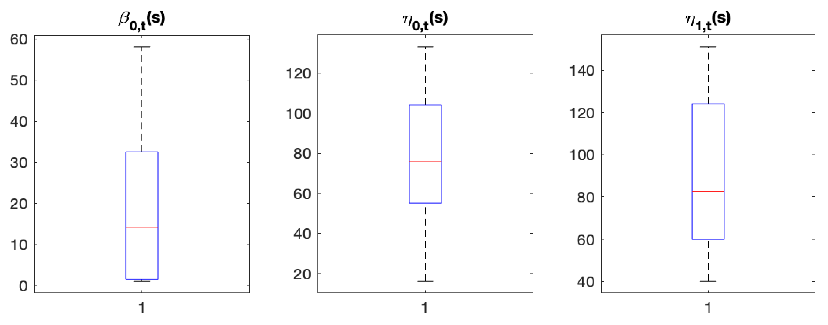
More Validation Results for Model-1c. We first check the number of distinct model parameters for Model-1c. Figure A5 shows the boxplots of the numbers of distinct values for the and -coefficients. We can see that the numbers of distinct coefficients are small relative to the sample size (which is ), with median values less than 100. The largest number of model parameters of the fitted ST-LAR models is about 300, which is much smaller than the sample size. Therefore, the model we choose (Model-1c) does not obviously suffer from over-fitting.
Figure A5.
Boxplots of the numbers of distinct coefficients at years 2001–2020 for Model-1c.

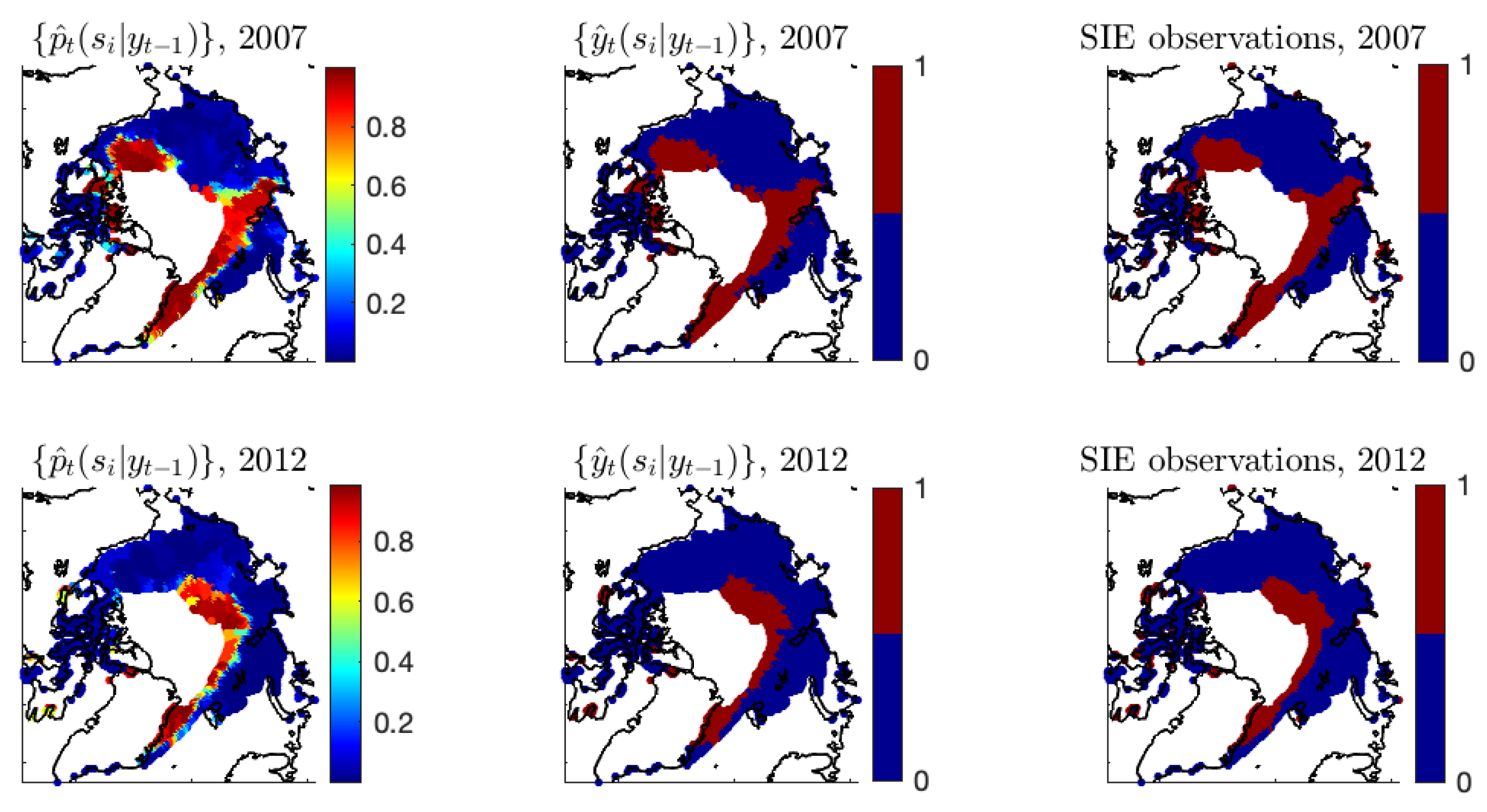
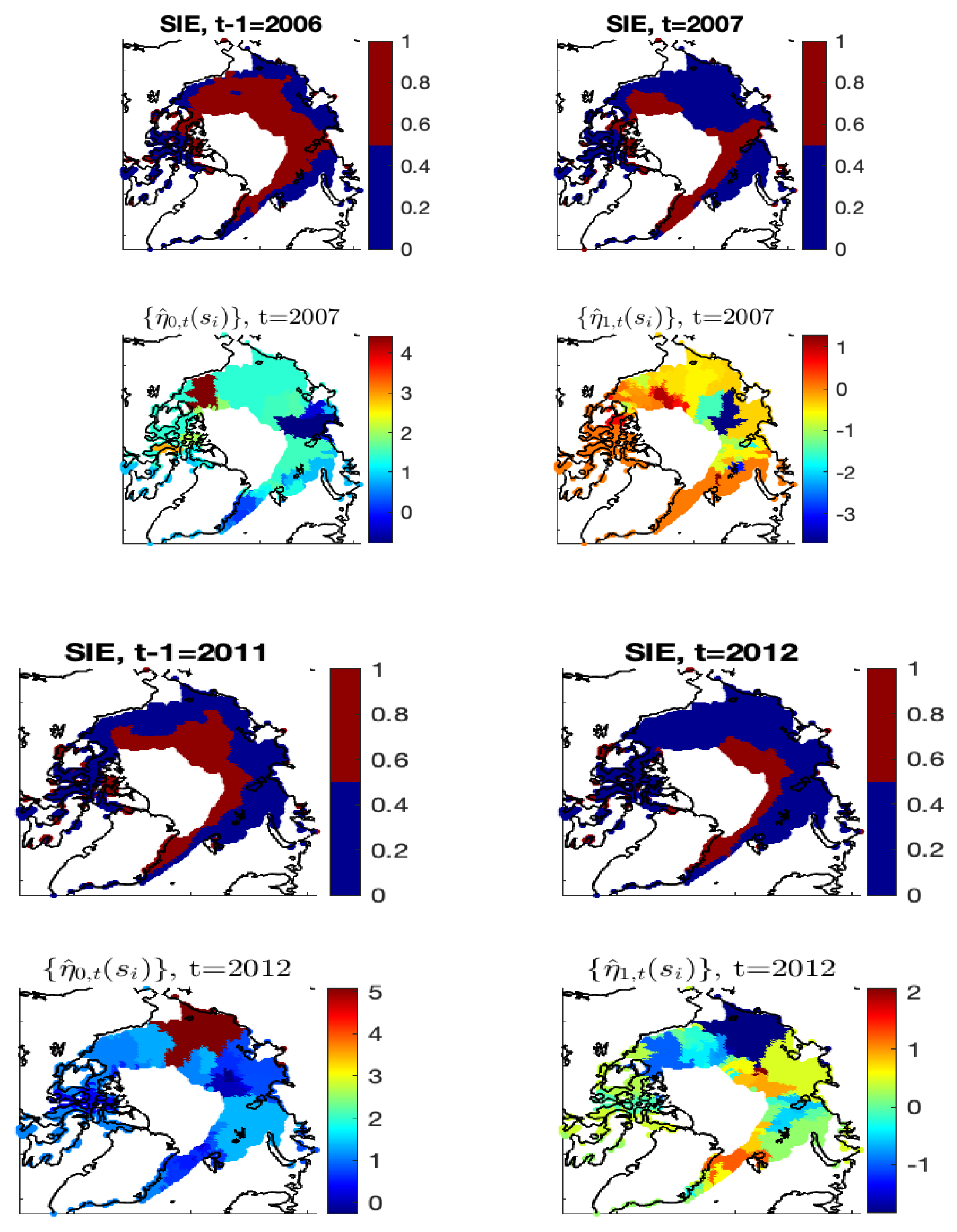
Figure A6 shows the additional estimation results of Model-1c at and 2012. We can see that the fitted results from Model-1c are reasonable, resulting in the estimated ice probabilities behaving similarly to the Arctic SIE data. The corresponding estimates of the autoregressive coefficients are shown in Figure A7, whose values adapt well to the observed ice–water/water–ice transitions in regions with substantial loss or gain of sea ice from to t.
Figure A6.
Years 2007 and 2012 are shown. Left panels: The estimates . Middle panels: The estimates using a cut-off value to dichotomize . Right panels: The binary Arctic sea ice data derived from satellite data.
Figure A6.
Years 2007 and 2012 are shown. Left panels: The estimates . Middle panels: The estimates using a cut-off value to dichotomize . Right panels: The binary Arctic sea ice data derived from satellite data.

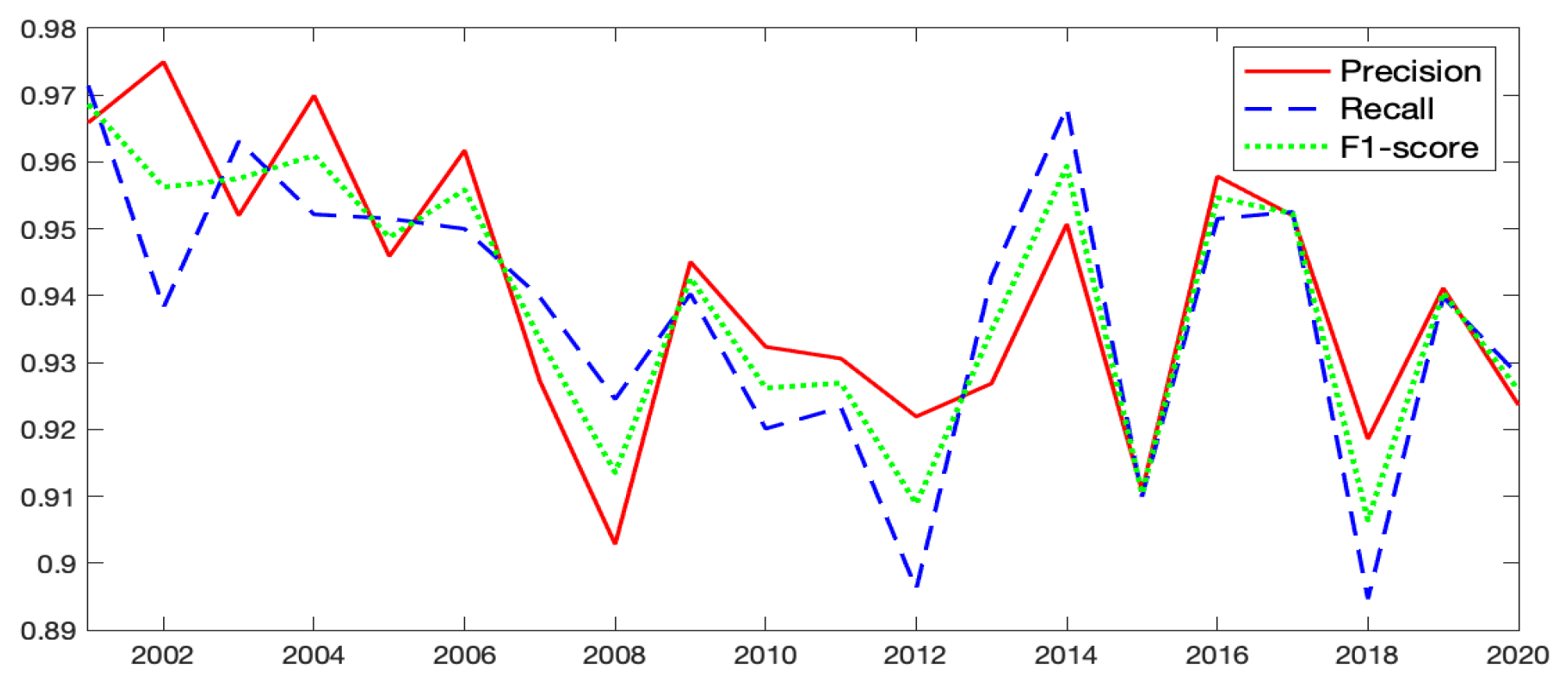
The time-averaged confusion matrix is given in Table A4. The number of misclassified ice grid cells and the number of misclassified water grid cells are roughly balanced. The time-averaged correct classification rate for ice is , which is very close to that for water (). We further calculated several parameters of the confusion matrix for the selected Model-1c, including precision, recall (sensitivity), and F1-score. Precision is the proportion of correctly classified ice grid cells among all the classified ice grid cells by the model, recall is the proportion of correctly classified ice grid cells among all the observed ice grid cells, and F1-score is the harmonic mean of precision and recall.
Figure A7.
Spatial maps of the observed ice/water statuses at and t and the autoregressive-coefficient estimates and of Model-1c, for and .
Figure A7.
Spatial maps of the observed ice/water statuses at and t and the autoregressive-coefficient estimates and of Model-1c, for and .

Table A4.
Time-averaged confusion matrix for Model-1c.
| (actual ice) | ||
| (actual water) |
The corresponding time series plots of those parameters for Model-1c are shown in Figure A8. The time series of the precision, recall, and F1-score parameters have fluctuations over years, with values generally above . We find that relatively lower values of precision and recall occur at years when the overall sea ice patterns are largely different between and t (e.g., and 2018). This may be because when the sea ice patterns change dramatically from to t, it will be difficult to borrow last year’s sea ice information to estimate the presence of sea ice in the current year.
Figure A8.
The time series of precision, recall, and F1-score parameters of the confusion matrix for Model-1c.
Figure A8.
The time series of precision, recall, and F1-score parameters of the confusion matrix for Model-1c.

Last, we have conducted an experiment to test the spatial prediction performance of Model-1c. Specifically, we randomly split the data locations into a training set with 7806 locations and a testing set with 867 locations; the training set contains about of the total locations, and the testing set contains the remaining . At each time point t, we first estimated the model parameters based on the training data, and spatial predictions were conducted subsequently by (i) obtaining the autoregressors for each testing location using its 8 nearest neighboring training data at time and (ii) plugging in the estimated model coefficients corresponding to the training data that are nearest to . In this way, we can obtain estimated ice probabilities for the testing data. The following Table A5 gives the time-averaged model evaluation scores of Model-1c on both the training and testing data. We can see that the estimation results for the best model (Model-1c) are still reasonable, with the three model evaluation scores for the testing data close to those for the training data.
Table A5.
Time-averaged model evaluation scores: The mean squared errors (MSEs), Nash–Sutcliffe model efficiency coefficients (NSEs), and the correct classification rates (CRs) for Model-1c.
Table A5.
Time-averaged model evaluation scores: The mean squared errors (MSEs), Nash–Sutcliffe model efficiency coefficients (NSEs), and the correct classification rates (CRs) for Model-1c.
| Model-1c | MSE | NSE | CR |
|---|---|---|---|
| Training | |||
| Testing |
Conclusion. Our conclusion is that Model-1c, namely, the model given by (3) in the paper, is the best model. Its estimates give superior model evaluation scores, and hence those estimates are used to compute the summaries and their visualization of the spatio-temporal variability in Arctic sea ice.
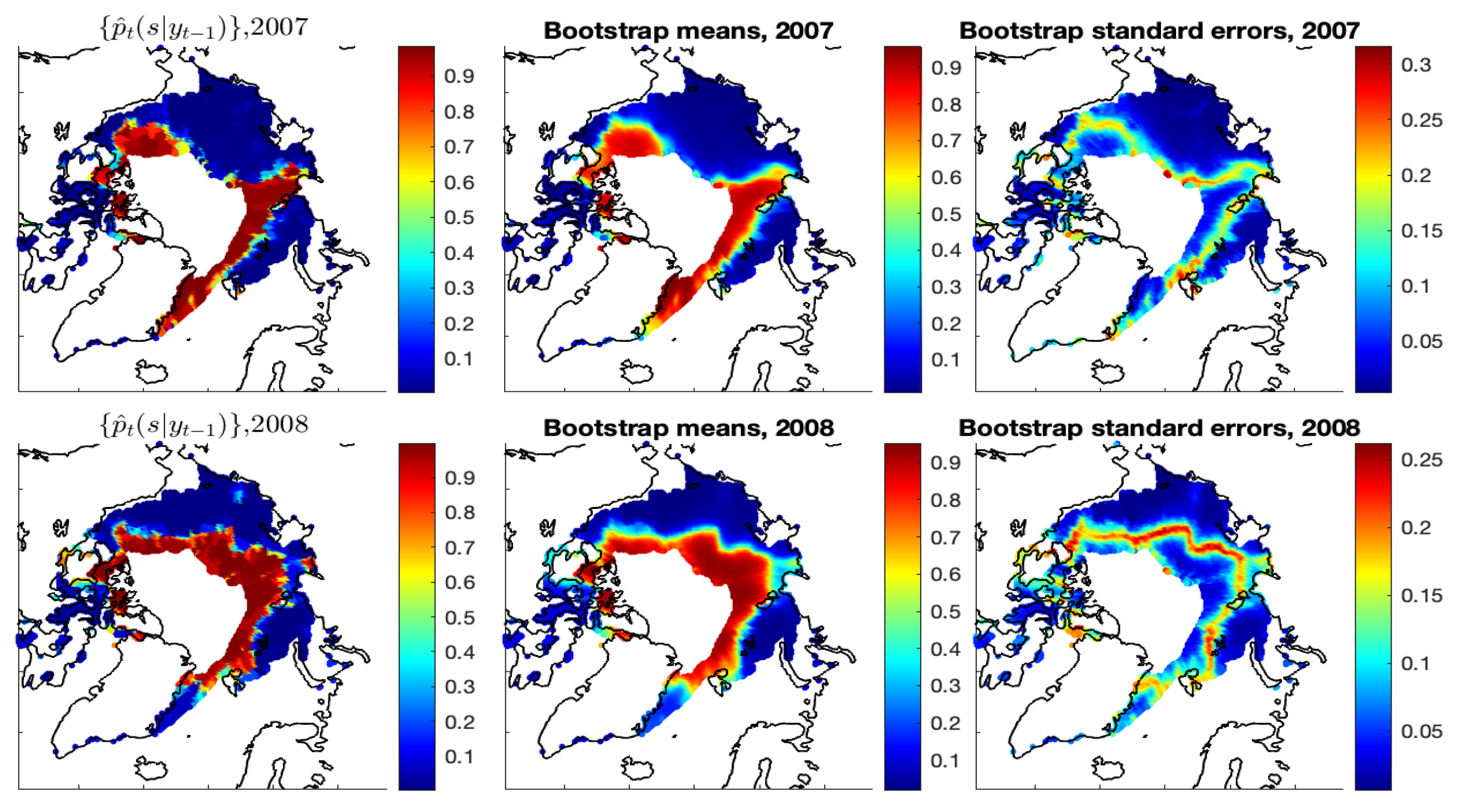
Uncertainty Estimation. The parametric bootstrap method, e.g., [54] provides a feasible way for obtaining the standard errors of for Model-1c. Let denote the parameter estimates of Model-1c at time t. The bootstrap samples can be generated in the following manner. At the initial time , the estimates are plugged into equation (3) to obtain the estimated ice probabilities , and the bootstrap samples, , are independently generated from the Bernoulli distributions with parameters . Then, starting from , the bootstrap samples at time t are generated by (i) constructing the autoregressors using the bootstrap samples ; (ii) plugging the autoregressors and the parameter estimates into (3) to obtain the estimated ice probabilities ; and (iii) generating the bootstrap samples independently from the Bernoulli distributions with parameters . This data-generating process is repeated B times to obtain B bootstrap samples.
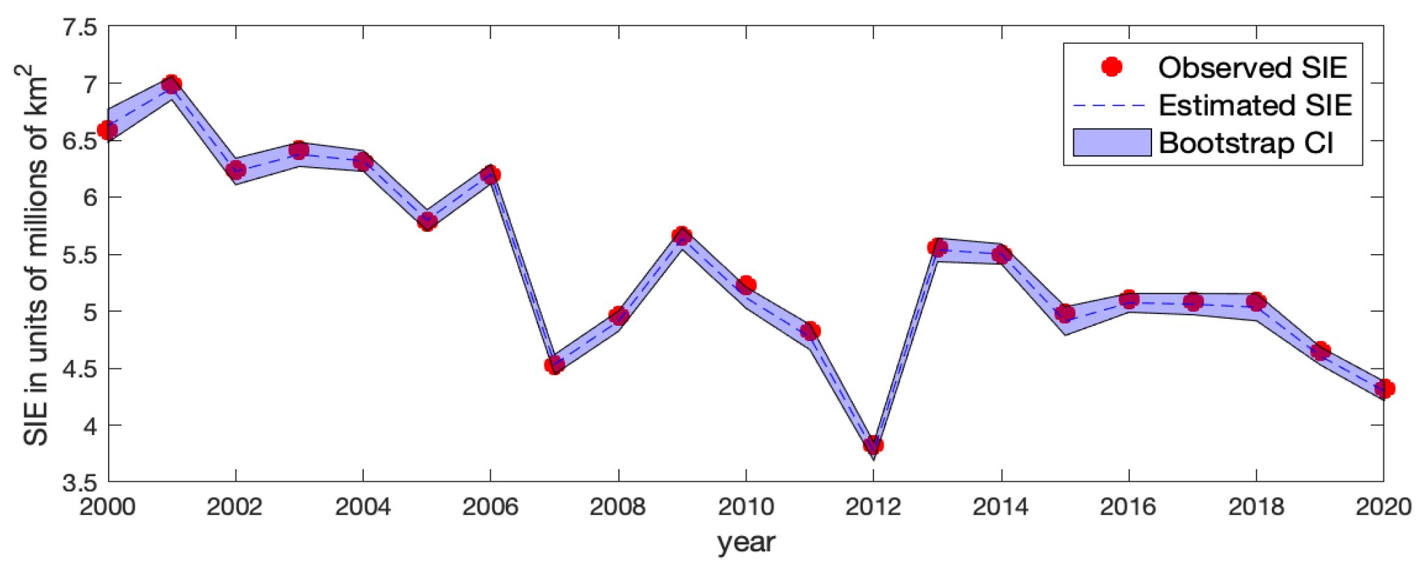
The right panels of Figure A9 show the bootstrap standard errors of the estimated ice probabilities of Model-1c based on 100 bootstrap samples. We can see that the uncertainties of mainly reside in the ice–water boundary regions where classifying ice/water grid cells is more difficult. We also obtained the standard errors of the estimated Arctic SIE based on those bootstrap samples at each year t. The corresponding approximate confidence interval of the Arctic SIE is shown in Figure A10, where at each time t, the upper and lower limits of the bootstrap confidence interval are equal to the estimated Arctic SIE plus and minus its two bootstrap standard errors, respectively. Values at time are joined to respective values at time t by straight lines. The pointwise bootstrap confidence intervals generally cover the observed Arctic SIE values, indicating that the fitting results are reasonable.
Figure A9.
Years 2007 and 2008 are shown. Left panels: The estimates of Model-1c. Middle panels: The bootstrap means of the estimated ice probabilities from 100 bootstrap samples. Right panels: The bootstrap standard errors of the estimated ice probabilities.
Figure A9.
Years 2007 and 2008 are shown. Left panels: The estimates of Model-1c. Middle panels: The bootstrap means of the estimated ice probabilities from 100 bootstrap samples. Right panels: The bootstrap standard errors of the estimated ice probabilities.

Figure A10.
The observed Arctic SIE (red solid dot), the estimated Arctic SIE by Model-1c (blue dashed line), and the bootstrap pointwise confidence interval of the Arctic SIE (shaded blue band).
Figure A10.
The observed Arctic SIE (red solid dot), the estimated Arctic SIE by Model-1c (blue dashed line), and the bootstrap pointwise confidence interval of the Arctic SIE (shaded blue band).

References
- Parkinson, C.L.; Cavalieri, D.J.; Gloersen, P.; Zwally, H.J.; Comiso, J.C. Arctic sea ice extents, areas, and trends, 1978–1996. J. Geophys. Res. Ocean. 1999, 104, 20837–20856. [Google Scholar] [CrossRef]
- Comiso, J.C.; Parkinson, C.L.; Gersten, R.; Stock, L. Accelerated decline in the Arctic sea ice cover. Geophys. Res. Lett. 2008, 35, L01703. [Google Scholar] [CrossRef] [Green Version]
- Cavalieri, D.J.; Parkinson, C.L. Arctic sea ice variability and trends, 1979–2010. Cryosphere 2012, 6, 881–889. [Google Scholar] [CrossRef] [Green Version]
- Parkinson, C.L. Global sea ice coverage from satellite data: Annual cycle and 35-yr trends. J. Clim. 2014, 27, 9377–9382. [Google Scholar] [CrossRef] [Green Version]
- Parkinson, C.L. Spatially mapped reductions in the length of the Arctic sea ice season. Geophys. Res. Lett. 2014, 41, 4316–4322. [Google Scholar] [CrossRef] [PubMed] [Green Version]
- Parkinson, C.L.; DiGirolamo, N.E. New visualizations highlight new information on the contrasting Arctic and Antarctic sea-ice trends since the late 1970s. Remote Sens. Environ. 2016, 183, 198–204. [Google Scholar] [CrossRef] [Green Version]
- Stroeve, J.; Notz, D. Changing state of Arctic sea ice across all seasons. Environ. Res. Lett. 2018, 13, 103001. [Google Scholar] [CrossRef]
- Meier, W.N.; Stroeve, J. An updated assessment of the changing Arctic sea ice cover. Oceanography 2022, 35, 1–10. [Google Scholar] [CrossRef]
- Curry, J.A.; Schramm, J.L.; Ebert, E.E. Sea ice-albedo climate feedback mechanism. J. Clim. 1995, 8, 240–247. [Google Scholar] [CrossRef]
- Kumar, A.; Perlwitz, J.; Eischeid, J.; Quan, X.; Xu, T.; Tao, Z.; Hoerling, M.; Jha, B.; Wang, W. Contribution of sea ice loss to Arctic amplification. Geophys. Res. Lett. 2010, 37, 389–400. [Google Scholar] [CrossRef]
- Pistone, K.; Eisenman, I.; Ramanathan, V. Observational determination of albedo decrease caused by vanishing Arctic sea ice. Proc. Natl. Acad. Sci. USA 2014, 111, 3322–3326. [Google Scholar] [CrossRef] [PubMed] [Green Version]
- Screen, J.A.; Simmonds, I. Exploring links between Arctic amplification and mid-latitude weather. Geophys. Res. Lett. 2013, 40, 959–964. [Google Scholar] [CrossRef] [Green Version]
- Mori, M.; Watanabe, M.; Shiogama, H.; Inoue, J.; Kimoto, M. Robust Arctic sea-ice influence on the frequent Eurasian cold winters in past decades. Nat. Geosci. 2014, 7, 869–873. [Google Scholar] [CrossRef]
- Cohen, J.; Screen, J.A.; Furtado, J.C.; Barlow, M.; Whittleston, D.; Coumou, D.; Francis, J.; Dethloff, K.; Entekhabi, D.; Overland, J.; et al. Recent Arctic amplification and extreme mid-latitude weather. Nat. Geosci. 2014, 7, 627–637. [Google Scholar] [CrossRef] [Green Version]
- Cvijanovic, I.; Santer, B.D.; Bonfils, C.; Lucas, D.D.; Jch, C.; Zimmerman, S. Future loss of Arctic sea-ice cover could drive a substantial decrease in California’s rainfall. Nat. Commun. 2017, 8, 1947. [Google Scholar] [CrossRef] [Green Version]
- Blackport, R.; Screen, J.A. Influence of Arctic sea ice loss in autumn compared to that in winter on the atmospheric circulation. Geophys. Res. Lett. 2019, 46, 2213–2221. [Google Scholar] [CrossRef] [Green Version]
- Olonscheck, D.; Mauritsen, T.; Notz, D. Arctic sea-ice variability is primarily driven by atmospheric temperature fluctuations. Nat. Geosci. 2019, 12, 430–434. [Google Scholar] [CrossRef]
- Labe, Z.; Peings, Y.; Magnusdottir, G. Contributions of ice thickness to the atmospheric response from projected Arctic sea ice loss. Geophys. Res. Lett. 2018, 45, 5635–5642. [Google Scholar] [CrossRef] [Green Version]
- Wernli, H.; Papritz, L. Role of polar anticyclones and mid-latitude cyclones for Arctic summertime sea-ice melting. Nat. Geosci. 2018, 11, 108–113. [Google Scholar] [CrossRef]
- Zhan, Y.; Davies, R. September Arctic sea ice extent indicated by June reflected solar radiation. J. Geophys. Res. Atmos. 2017, 122, 2194–2202. [Google Scholar] [CrossRef]
- Meier, W.N.; Fetterer, F.; Windnagel, A.K.; Stewart, J.S. NOAA/NSIDC Climate Data Record of Passive Microwave Sea Ice Concentration, Version 4 [Data Set]. 2021. Available online: https://nsidc.org/data/g02202/versions/4 (accessed on 16 August 2022). [CrossRef]
- Zhang, B.; Cressie, N. Estimating spatial changes over time of Arctic sea ice using hidden 2 × 2 tables. J. Time Ser. Anal. 2019, 40, 288–311. [Google Scholar] [CrossRef] [Green Version]
- Zhang, B.; Cressie, N. Bayesian inference of spatio-temporal changes of Arctic sea ice. Bayesian Anal. 2020, 15, 605–631. [Google Scholar] [CrossRef]
- Dempster, A.P.; Laird, N.M.; Rubin, D.B. Maximum likelihood from incomplete data via the EM algorithm. J. R. Stat. Soc. Ser. B (Methodol.) 1977, 39, 1–22. [Google Scholar]
- Horvath, S.; Stroeve, J.; Rajagopalan, B.; Kleiber, W. A Bayesian logistic regression for probabilistic forecasts of the minimum September Arctic sea ice cover. Earth Space Sci. 2020, 7, e2020EA001176. [Google Scholar] [CrossRef]
- Chang, W.; Haran, M.; Applegate, P.; Pollard, D. Calibrating an ice sheet model using high-dimensional binary spatial data. J. Am. Stat. Assoc. 2016, 111, 57–72. [Google Scholar] [CrossRef] [Green Version]
- Chang, W.; Haran, M.; Applegate, P.; Pollard, D. Improving ice sheet model calibration using paleoclimate and modern data. Ann. Appl. Stat. 2016, 10, 2274–2302. [Google Scholar] [CrossRef]
- Director, H.M.; Raftery, A.E.; Bitz, C.M. Improved sea ice forecasting through spatiotemporal bias correction. J. Clim. 2017, 30, 9493–9510. [Google Scholar] [CrossRef]
- Director, H.M.; Raftery, A.E.; Bitz, C.M. Probabilistic forecasting of the Arctic sea ice edge with contour modeling. Ann. Appl. Stat. 2021, 15, 711–726. [Google Scholar] [CrossRef]
- Cressie, N. Statistics for Spatial Data, Revised Edition; John Wiley & Sons: Hoboken, NJ, USA, 1993. [Google Scholar]
- Besag, J. Spatial interaction and the statistical analysis of lattice systems. J. R. Stat. Soc. Ser. B (Stat. Methodol.) 1974, 36, 192–225. [Google Scholar] [CrossRef]
- Caragea, P.C.; Kaiser, M.S. Autologistic models with interpretable parameters. J. Agric. Biol. Environ. Stat. 2009, 14, 281–300. [Google Scholar] [CrossRef]
- Shin, Y.E.; Sang, H.; Liu, D.; Ferguson, T.A.; Song, P.X. Autologistic network model on binary data for disease progression study. Biometrics 2019, 75, 1310–1320. [Google Scholar] [CrossRef] [PubMed]
- Zhu, J.; Huang, H.C.; Wu, J. Modeling spatial-temporal binary data using Markov random model. J. Agric. Biol. Environ. Stat. 2005, 10, 212–225. [Google Scholar] [CrossRef] [Green Version]
- Zheng, Y.; Zhu, J. Markov chain Monte Carlo for a spatial-temporal autologistic regression model. J. Comput. Graph. Stat. 2008, 17, 123–137. [Google Scholar] [CrossRef]
- Zhu, J.; Zheng, Y.; Carroll, A.L.; Aukema, B.H. Autologistic regression analysis of spatial-temporal binary data via Monte Carlo maximum likelihood. J. Agric. Biol. Environ. Stat. 2008, 13, 84–98. [Google Scholar] [CrossRef]
- Diggle, P.J.; Tawn, J.; Moyeed, R. Model-based geostatistics (with discussion). J. R. Stat. Soc. Ser. C (Appl. Stat.) 1998, 47, 299–350. [Google Scholar] [CrossRef]
- Sengupta, A.; Cressie, N. Hierarchical statistical modeling of big spatial datasets using the exponential family of distributions. Spat. Stat. 2013, 4, 14–44. [Google Scholar] [CrossRef] [Green Version]
- Chu, T.; Zhu, J.; Wang, H. Penalized maximum likelihood estimation and variable selection in geostatistics. Ann. Stat. 2011, 39, 2607–2625. [Google Scholar] [CrossRef]
- Li, F.; Sang, H. Spatial homogeneity pursuit of regression coefficients for large datasets. J. Am. Stat. Assoc. 2019, 114, 1050–1062. [Google Scholar] [CrossRef]
- Cavalieri, D.J.; Gloersen, P.; Campbell, W.J. Determination of sea ice parameters with the Nimbus 7 SMMR. J. Geophys. Res. Atmos. 1984, 89, 5355–5369. [Google Scholar] [CrossRef]
- Comiso, J.C. Characteristics of Arctic winter sea ice from satellite multispectral microwave observations. J. Geophys. Res. Ocean. 1986, 91, 975–994. [Google Scholar] [CrossRef]
- Zwally, H.J.; Comiso, J.C.; Parkinson, C.L.; Cavalieri, D.J.; Gloersen, P. Variability of Antarctic sea ice 1979–1998. J. Geophys. Res. Ocean. 2002, 107, 9-1–9-19. [Google Scholar] [CrossRef] [Green Version]
- Meier, W.N.; Stroeve, J.; Fetterer, F. Whither Arctic sea ice? A clear signal of decline regionally, seasonally and extending beyond the satellite record. Ann. Glaciol. 2007, 46, 428–434. [Google Scholar] [CrossRef] [Green Version]
- Kato, S.; Rose, F.G.; Rutan, D.A.; Thorsen, T.J.; Loeb, N.G.; Doelling, D.R.; Huang, X.; Smith, W.L.; Su, W.; Ham, S.H. Surface irradiances of edition 4.0 Clouds and the Earth’s Radiant Energy system (CERES) Energy Balanced and Filled (EBAF) data product. J. Clim. 2018, 31, 4501–4527. [Google Scholar] [CrossRef]
- Loeb, N.G.; Doelling, D.R.; Wang, H.; Su, W.; Nguyen, C.; Corbett, J.G.; Liang, L.; Mitrescu, C.; Rose, F.G.; Kato, S. Clouds and the Earth’s Radiant Energy System (CERES) Energy Balanced and Filled (EBAF) top-of-atmosphere (TOA) edition-4.0 data product. J. Clim. 2018, 31, 895–918. [Google Scholar] [CrossRef]
- NASA/LARC/SD/ASDC. CERES Time-Interpolated TOA Fluxes, Clouds and Aerosols Monthly Aqua Edition4A. 2015. Available online: https://asdc.larc.nasa.gov/project/CERES/CER_SSF1deg-Month_Aqua-MODIS_Edition4A (accessed on 7 August 2022). [CrossRef]
- Minnis, P.; Trepte, Q.Z.; Sun-Mack, S.; Chen, Y.; Doelling, D.R.; Young, D.F.; Spangenberg, D.A.; Miller, W.F.; Wielicki, B.A.; Brown, R.R.; et al. Cloud detection in nonpolar regions for CERES using TRMM VIRS and Terra and Aqua MODIS data. IEEE Trans. Geosci. Remote Sens. 2008, 46, 3857–3884. [Google Scholar] [CrossRef]
- Minnis, P.; Sun-Mack, S.; Young, D.F.; Heck, P.W.; Garber, D.P.; Chen, Y.; Spangenberg, D.A.; Arduini, R.F.; Trepte, Q.Z.; Smith, W.L.; et al. CERES edition-2 cloud property retrievals using TRMM VIRS and Terra and Aqua MODIS data—Part I: Algorithms. IEEE Trans. Geosci. Remote Sens. 2011, 49, 4374–4400. [Google Scholar] [CrossRef]
- Sun-Mack, S.; Minnis, P.; Chen, Y.; Doelling, D.R.; Scarino, B.R.; Haney, C.O.; Smith, W.L. Calibration changes to Terra MODIS Collection-5 radiances for CERES Edition 4 cloud retrievals. IEEE Trans. Geosci. Remote Sens. 2018, 56, 6016–6032. [Google Scholar] [CrossRef] [PubMed]
- Tibshirani, R.; Saunders, M.; Rosset, S.; Zhu, J.; Knight, K. Sparsity and smoothness via the fused LASSO. J. R. Stat. Soc. Ser. B (Stat. Methodol.) 2005, 67, 91–108. [Google Scholar] [CrossRef] [Green Version]
- Brier, G.W. Verification of forecasts expressed in terms of probability. Mon. Weather Rev. 1950, 78, 1–3. [Google Scholar] [CrossRef]
- Nash, J.E.; Sutcliffe, J.V. River flow forecasting through conceptual models part I—A discussion of principles. J. Hydrol. 1970, 10, 282–290. [Google Scholar] [CrossRef]
- Efron, B.; Tibshirani, R.J. An Introduction to the Bootstrap; Chapman & Hall/CRC Press: Boca Raton, FL, USA, 1994. [Google Scholar]
- Blanchard-Wrigglesworth, E.; Armour, K.C.; Bitz, C.M.; DeWeaver, E. Persistence and inherent predictability of Arctic sea ice in a GCM ensemble and observations. J. Clim. 2011, 24, 231–250. [Google Scholar] [CrossRef]
- Besag, J. Statistical analysis of non-lattice data. J. R. Stat. Soc. Ser. D (Stat.) 1975, 24, 179–195. [Google Scholar] [CrossRef] [Green Version]
- Lee, D.T.; Schachter, B.J. Two algorithms for constructing a Delaunay triangulation. Int. J. Comput. Inf. Sci. 1980, 9, 219–242. [Google Scholar] [CrossRef]
- Akaike, H. A new look at the statistical model identification. IEEE Trans. Autom. Control 1974, 19, 716–723. [Google Scholar] [CrossRef]
- Schwarz, G. Estimating the dimension of a model. Ann. Stat. 1978, 6, 461–464. [Google Scholar] [CrossRef]
Figure 1.
The observed Arctic SIE from 2000 to 2020, with a fitted linear regression line (blue dashed line) using year t as a single covariate.
Figure 1.
The observed Arctic SIE from 2000 to 2020, with a fitted linear regression line (blue dashed line) using year t as a single covariate.

Figure 2.
Boxplots of ice proportions in different latitude bands centered at . The average of ice proportions is represented by a dot (•) and the horizontal bars in the boxplots show the five-number summaries of a distribution (namely, minimum, first quartile, median, third quartile, and maximum). The five-year-interval boxplots are shaded from blue (2000) through green (2010) to red (2020).

Figure 3.
Left panel: The Arctic sea ice concentrations in September of 2001. Right panel: The corresponding binary Arctic SIE data in the same month. The spatial grid cells are displayed in a polar stereographic projection.
Figure 3.
Left panel: The Arctic sea ice concentrations in September of 2001. Right panel: The corresponding binary Arctic SIE data in the same month. The spatial grid cells are displayed in a polar stereographic projection.

Figure 4.
The spatial grid cells (in red) with at least one observed ice–water or water–ice transition from 2000 to 2020.
Figure 4.
The spatial grid cells (in red) with at least one observed ice–water or water–ice transition from 2000 to 2020.

Figure 5.
The time series of spatially averaged CS-RSR data for June (blue dashed line) versus the Arctic SIE data for September (red solid line). The averaged values of RSR are taken over all RSR observations in the Arctic region (latitudes N).
Figure 5.
The time series of spatially averaged CS-RSR data for June (blue dashed line) versus the Arctic SIE data for September (red solid line). The averaged values of RSR are taken over all RSR observations in the Arctic region (latitudes N).

Figure 6.
Spatio-temporal representation of the autoregressive structure, where the black square indicates the spatial domain, the colored circles indicate spatial locations, the solid black lines in the black square define the neighborhood of those spatial locations, and the dashed colored lines define the autoregressive dependence at location . Circles corresponding to water (ice) grid cells are colored blue (red).

Figure 7.
Years 2008 and 2013 are shown. Left panels: The estimates . Middle panels: The estimates using a cut-off value to dichotomize . Right panels: The binary Arctic sea ice data derived from satellite data.
Figure 7.
Years 2008 and 2013 are shown. Left panels: The estimates . Middle panels: The estimates using a cut-off value to dichotomize . Right panels: The binary Arctic sea ice data derived from satellite data.

Figure 8.
Spatial maps of the autoregressive-coefficient estimates and for the best model at and .

Figure 9.
Observed Arctic SIE (red solid line) versus the estimated Arctic SIE based on the model given by (3) (blue dashed line).
Figure 9.
Observed Arctic SIE (red solid line) versus the estimated Arctic SIE based on the model given by (3) (blue dashed line).

Figure 10.
Boxplots of the estimates from the model given by (3) for different latitude bands with half-bandwidth . The horizontal dashed line indicates a probability, and the solid dots indicate the averaged values of . The horizontal bars in the boxplots show the five-number summaries of a distribution (namely, minimum, first quartile, median, third quartile, and maximum). The five-year-interval boxplots are shaded from blue (2000) through green (2010) to red (2020).

Publisher’s Note: MDPI stays neutral with regard to jurisdictional claims in published maps and institutional affiliations. |
© 2022 by the authors. Licensee MDPI, Basel, Switzerland. This article is an open access article distributed under the terms and conditions of the Creative Commons Attribution (CC BY) license (https://creativecommons.org/licenses/by/4.0/).
Share and Cite
MDPI and ACS Style
Zhang, B.; Li, F.; Sang, H.; Cressie, N. Inferring Changes in Arctic Sea Ice through a Spatio-Temporal Logistic Autoregression Fitted to Remote-Sensing Data. Remote Sens. 2022, 14, 5995. https://0-doi-org.brum.beds.ac.uk/10.3390/rs14235995
AMA Style
Zhang B, Li F, Sang H, Cressie N. Inferring Changes in Arctic Sea Ice through a Spatio-Temporal Logistic Autoregression Fitted to Remote-Sensing Data. Remote Sensing. 2022; 14(23):5995. https://0-doi-org.brum.beds.ac.uk/10.3390/rs14235995
Chicago/Turabian StyleZhang, Bohai, Furong Li, Huiyan Sang, and Noel Cressie. 2022. "Inferring Changes in Arctic Sea Ice through a Spatio-Temporal Logistic Autoregression Fitted to Remote-Sensing Data" Remote Sensing 14, no. 23: 5995. https://0-doi-org.brum.beds.ac.uk/10.3390/rs14235995
Note that from the first issue of 2016, this journal uses article numbers instead of page numbers. See further details here.