Article

An Empirical Bayesian Approach to Quantify Multi-Scale Spatial Structural Diversity in Remote Sensing Data

1
Department of Mathematics, University of Zurich, 8057 Zürich, Switzerland
2
Department of Geography, University of Zurich, 8057 Zürich, Switzerland
3
Remote Sensing Laboratories, Department of Geography, University of Zurich, 8057 Zürich, Switzerland
4
Institute of Computational Science, University of Zurich, 8006 Zürich, Switzerland
*
Author to whom correspondence should be addressed.
Submission received: 30 September 2022 / Revised: 9 December 2022 / Accepted: 13 December 2022 / Published: 21 December 2022

Abstract

:
Landscape structure is as much a driver as a product of environmental and biological interactions and it manifests as scale-specific, but also as multi-scale patterns. Multi-scale structure affects processes on smaller and larger scales and its detection requires information from different scales to be combined. Herein, we propose a novel method to quantify multi-scale spatial structural diversity in continuous remote sensing data. We combined information from different extents with an empirical Bayesian model and we applied a new entropy metric and a value co-occurrence approach to capture heterogeneity. We tested this method on Normalized Difference Vegetation Index data in northern Eurasia and on simulated data and we also tested the effect of coarser pixel resolution. We find that multi-scale structural diversity can reveal itself as patches and linear landscape features, which persist or become apparent across spatial scales. Multi-scale line features reveal the transition zones between spatial regimes and multi-scale patches reveal those areas within transition zones where values are most different from each other. Additionally, spatial regimes themselves can be distinguished. We also find the choice of scale need not be informed by typical length-scales, which makes the method easy to implement. The proposed multi-scale approach can be applied to other contexts, following the roadmap we pave out in this study and using the tools available in the accompanying R package StrucDiv.

1. Background

Landscape structure is closely linked to both climate change [1,2] and biodiversity loss [3,4], because it locates ecological, environmental and anthropogenic phenomena that shape the earth’s surface [5]. Spatial structural diversity—hereafter, structural diversity—refers to the arrangement of landscape elements in horizontal space. It is both an aspect of biodiversity [6], and a mediator of ecological processes [7]. Quantifying structural diversity is critical, because it indicates alterations in the extent and structure of the world’s biomes, including tundra and taiga [8,9]. In the northern high latitudes, climate change takes effect faster than in lower latitudes [10,11,12], which is particularly worrisome because boreal forests are among the largest carbon sinks and vast amounts of methane are stored in tundra soils. The transitioning of tundra and taiga biomes manifests through shifts in vegetation structure [13,14,15] and in mountainous regions, rising temperatures enable vegetation to migrate to higher altitudes [16]. While latitudinal and altitudinal vegetation change is an established climate change effect [17], quantification methods are somewhat behind. With the rise of remote sensing technology, unprecedented amounts of information are at our disposal [18], yet methods to assess landscape heterogeneity are still dominated by the ‘patch mosaic paradigm’. This means that most studies employ categorical land cover class (LCC) data [19,20], a reductionist approach that is only slowly being overcome [21,22].
Methods to quantify the diversity aspect of landscape structure frequently build upon the mathematical formulation of entropy [23,24,25], which is perhaps the most widely used measure of diversity in different ecological systems [26,27]. In the study at hand, we employ a new entropy metric designed to quantify structural diversity in continuous raster data [28]. Further, methods to assess landscape structure inevitably involve spatial scale, which largely determines which structures are detected. More commonly, landscapes are decomposed into hierarchical levels of scale [7,29]. In a less common approach, information from different scales is combined to detect structures that dominate on multiple scales [30,31]. Although such multi-scale landscape structures play an important role for ecological and environmental processes [32,33], quantification methods have received little attention. Herein, we propose a novel method to include spatial scale in the quantification of landscape heterogeneity in continuous data. We introduce an empirical Bayesian approach to combine information from hierarchical levels of scale and we employed the metric structural diversity entropy to quantify multi-scale structural diversity in continuous remote sensing data.
Spatial scale is inherent to the world we live in and its importance for remote sensing, landscape ecology, biodiversity research and for science as a whole has long been recognized [34,35]. Natural processes tend to be scale-dependent, meaning that they operate on some scales but not on others, and they tend to manifest as and interact with scale-dependent spatial structures [34,36]. The prominent concept of hierarchically ordered scales [30,31,37] is described by so-called scale breaks [29] that separate spatial scale domains [7]. These are the typical process-inherent scales that are characterized by no or monotonic change of patterns [34]. For example, animal body mass corresponds with scale breaks in landscape structure [29] and forest habitat was found separable into scale-domains [38]. Yet, interactions between environmental and biological processes occur across scales and landscape structure can be as much the outcome as the origin of such associations [39]. Reduced habitat heterogeneity and climate change increase the risk of environmental damage by pest species, for example due to bark beetle outbreaks, which are caused by interlinked ‘cross-scale drivers’ [40]. Biodiversity loss also affects ecosystem functioning across scales of time and space and largely due to anthropogenic influences [41]. Methodological advancements to account for associations across multiple scales are therefore timely contributions to oppose the inseparable ecological and environmental crises of the 21st century.
Ref. [30] suggested there be two fundamental ways to capture cross-scale interactions: in an ‘indirect’ approach, methods developed for one spatial scale are repeated on several scales, whereas a ‘direct’ approach incorporates multiple scales in its model formulation. For example, ref. [42] used step-wise multiple linear regression as an indirect approach to determine the scale on which soil fauna diversity was best explained by landscape structure. Nested windows were exploited in direct approaches to detect targets [43,44,45] and for classification [46]. Direct approaches to decompose landscape structure include scale space decomposition [22,47], Fourier-based textural ordination [21] and fractal-based approaches [48,49]. Bayesian methods offer flexibility in complicated hierarchical settings and although their use remains limited [50], they have been employed as direct approaches to address mismatches between process scales and pixel resolution [51] and to model species distributions when multiple drivers interact at multiple scales [50]. Although empirical Bayesian methods have a long history in statistics [52], their benefits for ecological and geostatistical applications have only more recently gained attention [53,54]. Both empirical and fully Bayesian methods are based on the fundamental idea that prior information ‘and new data are combined […] to produce posterior knowledge’ [55], while the empirical Bayesian approach can be interpreted as an approximation to a fully Bayesian one. The main distinction between the two is that in an empirical Bayesian model, specific parameters of the prior are estimated from the data instead of being integrated in the Bayesian framework [56,57]. This means that uncertainty estimation is compromised, although on the other hand, empirical Bayesian methods do not face issues of convergence of the sampled hyperparameter [58]. Moreover, computation is faster [57], which suggests a promising future in big data applications, such as earth observation.
In natural landscapes, certain structures can persist across multiple scales [59] and dominate environmental and ecological processes on both smaller and larger scales [32,33,60]. To ‘characterize the multiple-scale structure of a landscape’ [30], information from different levels must be combined. ‘Linear scale space and blob-feature detection’ [31,61] has been used to identify homogeneous features that emerge as ‘some structures persist through scale, while others disappear’ [31]. Because scale-specific structural diversity was previously found to emerge as landscape features, such as patches and linear features, we hypothesized some of these structures may endure across scales. In this study, the term spatial feature refers to ‘an area that is (i) detected with a certain method and (ii) composed of similar values, which are the output values of the method that was used to detect the feature’ [28]. We previously quantified scale-specific structural diversity in Normalized Difference Vegetation Index (NDVI) data, which is an established proxy for photosynthesis and hence for vegetation cover and productivity [62,63]. Our study region in the northern high latitudes depicts a distinct value gradient along a transect, which we established as the transition zone between two spatial regimes [28]. Structural diversity features originate from these transition zones, which gives reason to believe that these zones represent the underlying, scale-independent diverse structure that drives the emergence of scale-specific features. We will use the term multi-scale features to describe the phenomenon of landscape features that persist across scales and we hypothesized that multi-scale structural diversity features can be detected with the right method specifications and that these features reveal the transition zones between spatial regimes.
Ref. [57] underlined the suitability of empirical Bayesian approaches for ‘combining information’ from different publications involving the same study area and we exploited this ability, yet the information we combined originates from different spatial extents within the same study area. We chose data resolution based on previous studies of vegetation change in tundra and taiga biomes [8,62,63] and we tested the effect of different size extents and the sensitivity of feature detection to three ways of combining these extents. We integrated information from different spatial scales by nesting smaller, inner extents inside larger, outer ones and we combined information with a direct approach, using an empirical Bayesian model. We tested the influence of different extents in the study area where we previously detected scale-specific features [28,64] and we also quantified structural diversity in NDVI data of northern Eurasia. Additionally, we simulated data depicting random patches, random noise and a linear value gradient. We expected the edges between patches and the surrounding area to be detected as multi-scale structural diversity features. We call them edges, because the value change is abrupt. Further, we expected to detect no multi-scale features and also no scale-specific features in random noise data or in linear gradient data. We hypothesized that when inner and outer scale are of similar size, multi-scale features would be similar to scale-specific ones and when the outer scale is much larger than the inner scale, we expected features to appear in front of a relatively homogeneous background. We expected the size of features to depend on the size of the inner scale and with an increasingly large outer scale, we ultimately expected the feature type to remain constant, i.e., to persist across scales. A detailed list of expectations can be found in Section 2.7. We completed our analysis by testing the effect of different pixel resolutions.
With this study, we propose a new method to quantify landscape heterogeneity that persists across scales in continuous remote sensing data. We strive to ‘learn more about how scale affects pattern’ [65] and we hope to serve the remote sensing community and others who may benefit from statistical methods to detect multi-scale structural diversity features.

2. Methods

2.1. Study Region, Data and Software

Our study area of 241,332 km2 is situated between 66.63 ° to 68.61 ° North and 165.02 ° to 174.83 ° East in the tundra and taiga ecosystems of northern Siberia (Figure 1). The energy and the water balance connect vegetation, soil and atmosphere through manifold ecological processes, yet temperature and precipitation are the main environmental variables that govern the extent of the world’s biomes [66]. For this reason, we previously investigated spatial structure in NDVI and also in land surface temperature and latent heat. We included topography because the study region comprises a mountain, and land cover class data for additional information. Our analysis revealed that the value gradient in NDVI data corresponds to a transition zone between two spatial regimes, which we called bareland regime and vegetation regime. The bareland regime is located in high elevation areas on steep slopes and is characterized by low NDVI values, low temperatures and strong temperature gradients, high variability in latent heat and the predominant land cover types being bareland, moss, lichens and shrubs. The vegetation regime populates low elevation areas and is characterized by high NDVI, warmer temperatures and a balanced latent heat flux. The predominant land cover types are forest and grassland. The regimes are detectable because all data reveal what we call correspondent structure, which refers to similar spatial structure in the same places [28]. These regimes may also be called ecosystems [67]; however, we use the term regime because it can also describe simulated data. We used a biweekly NDVI time-series product from the MODIS sensor, averaged over the 2018 growing season [68] and we chose a pixel resolution of 1 km2, because it has been promoted to investigate vegetation changes in tundra and taiga habitat [8,62,63]. Although we conducted most tests on the study region, we also quantified multi-scale structural diversity for the whole of northern Eurasia (50 ° to 70 ° North and 25 ° West to 180 ° East), using the same data. We complemented the analysis with coarser resolution data of the study region, created with mean NDVI aggregation.
We obtained data from Google Earth Engine [69], geo-referenced to latitude and longitude and used the programming language R for all further data processing [70]. In the northern high latitudes, quality issues of satellite imagery commonly cause data gaps and we closed the few missing values with a local neighborhood average. For verification, we complemented our experiment with a simulation of three different types of spatial structure: random structure, randomly placed patches and a linear gradient (Figure 2A,B(a,c,e)). First, we defined random structure as the absence of auto-correlation; hence, the random structure simulation can be called a white noise image. Second, we simulated four randomly placed patches with a radius of 14 pixels. The surrounding area and the inside of patches were simulated to have random structure; hence, patches are distinguished from the surrounding area only by a value offset. Third, we simulated a linear north–south gradient. The images have 90 rows and columns and we simulated all three landscape structure types with 10 and 100 gray levels (GLs). We simulated a steep and abrupt value change between patches and the surrounding area, which means that both are comprised of 5 or 50 GLs, respectively. In random patch data, the patches and the surrounding area (simulated as random noise) can be interpreted as two spatial regimes, whereas random noise and linear gradient data comprise only one regime. We used the raster package for all basic handling of raster data, spam and fields for simulation [71,72,73] and we developed our own R package StrucDiv for scale-specific and multi-scale structural diversity quantification [74].

2.2. Structural Diversity

Shannon entropy ( i = 1 n p i log p i ) [75] has been applied to spatial contexts for decades [23,76] and all approaches have in common that spatial information must be contained in the probabilities p i . This issue has been tackled in various ways, mostly using categorical data [24,25,76]. We employed a method that considers structure through the spatial arrangement of co-occurrring values, based on [77]. Spatial arrangement is defined by the distance between two pixel values v i and v j and by the angle that specifies their relative positions [77,78]. We chose distance 1 and the direction-invariant option, which considers all angles (Figure S2), after confirming near-isotropy with semi-variograms. The frequencies of co-occuring values are gathered in the gray level co-occurrence matrix (GLCM), which is normalized by the total number of pixel pairs n in an area. Hence, i and j index positions in the GLCM, which contains the empirical co-occurrence probabilities of v i and v j (Figure S2). To detect scale-specific heterogeneity, structural diversity entropy is calculated on these empirical probabilities:
Structural diversity entropy = i , j = 1 m p i j ln p i j | v i v j | δ , δ { 0 , 1 , 2 } ,
with m being the number of GLs in the area under consideration. To combine information across scales, posterior probabilities p i j p o s t were employed, as explained in Section 2.3 and Section 2.4.
Structural diversity entropy contains Shannon entropy as a particular case ( δ = 0) [75], but it can further capture value differences ( δ { 1 , 2 } ). Shannon entropy operates only on probabilities associated with value pairs and can be interpreted as β structural diversity, while including within-pair differences enables the metric to quantify γ structural diversity (using the product). The second-order texture metrics contrast and dissimilarity can detect landscape features similar to those detected with structural diversity entropy specified with δ { 1 , 2 } ; however, they cannot detect line features, because they only capture α structural diversity [28]. We previously found that metric formulation, spatial scale and the number of GLs determine which type of structural diversity features are detected and we based our experimental design on these results [28] (Tables S2 and S4). Shannon entropy is sensitive to the number of GLs (i.e., unique values), which also affects computation [79]. Consequently, we reduced NDVI to 10 and to 100 GLs and tested all metric formulations and scales on both data.

2.3. Spatial Scale

We used data in raster format, which means that spatial scale is represented by data resolution, distance and extent [80]. Data resolution is based on previous research, distance is determined by values being direct neighbors and extent is the main subject of our experiment. We combined information from different extents in three ways, i.e., with three nesting schemes, which differ by the representation of the outer scale, and we employed both data-inherent and uninformed scales (Figure 3). This allowed us to test the sensitivity of feature detection to (i) the size of the outer scale, (ii) how the outer scale is positioned in relation to the inner scale and (iii) whether the outer scale must be chosen based on data-inherent scales. These aspects determine the level of knowledge about data-inherent scales required to implement the method and also computational effort.
The area within which pixel pair associations are considered represents the spatial scale on which scale-specific structural diversity is quantified. Hence, if the whole domain D R 2 is considered, one value is obtained, which represents structural diversity of the domain. To capture structures within the domain, we used square, overlapping moving windows MW u , u = 1 , , w with w being the number of pixels in the domain. Moving windows shift by one pixel at a time and the size of MW u is defined by the window side length (WSL). The WSL is in units pixel, which here is the same as km. The WSL is an odd number; hence, moving windows are centered on one pixel and this center pixel receives the structural diversity value. The output map is called structural diversity map and it depicts scale-specific structural diversity in D , quantified on the scale WSL × WSL.
The inner scale was always defined by moving windows. Inner moving windows (MW I , u ) were placed inside larger, outer extents and we used pixel co-occurrences on the outer scale as prior information. First, we used double moving windows, meaning that we nested MW I , u inside larger, outer moving windows MW O , u (Figure 3a). Hence, the prior information for each pixel is retrieved from an area that is placed perfectly around the pixel. Second, we nested MW I , u inside stationary blocks B e , e = 1 , , f , meaning that blocks do not move. The domain is separated into several square blocks and windows move inside each block. This means that block and window are not centered on the same pixel and inside every B e , all windows are informed by the same prior (Figure 3b). Last, we used D as the prior scale for all MW I , u (Figure 3c).
When the nesting scheme relies on blocks, the output map can depict edges between them. To reduce this edge effect, we separated D into blocks in such a way that B e overlap with each other and when we merged the blocks back together (after structural diversity had been quantified), we did this in a spatially weighted manner. More specifically, we merged blocks with a linear weight between zero and one. Moving windows create edges with missing values (NA-edges) when they reach the edges of B e or D . The size of the NA-edge is determined by the WSL of the moving window (NA-edge-width = 0.5 × (WSL − 1)). When MW I , u were nested inside D , we treated NA-edges the same way as we treated them in the uni-scale approach—we removed them. This means that the structural diversity map is smaller than the input raster. When double moving windows are used, it is the WSL of the outer window that defines the width of the NA-edge. The NA-edge around blocks restricts the overlap, which must be WSL I 1 overlap 0.5 × WSL B . When blocks of specified size and overlap are fitted inside the domain, there may be edges that are too small to fit another block. These edges were cut off, which leads to different size structural diversity maps.
We based the choice of scales on typical scales on which structural diversity features were previously detected and on feature-inherent scales which we obtained with semi-variogram and effective range estimation (Tables S2 and S3). Line features were detected with structural diversity entropy using δ = 0 and an ideal WSL range of 5–11. Narrow line features, also called borders, were detected with δ = 2 and WSL 3–5. Different size patch features were detected with δ { 1 , 2 } and WSL 7–19 (Table S2). We defined inner scales accordingly, with WSL I { 3 , 7 , 13 } and outer scales with WSL O { 7 , 13 , 19 , 35 } . WSL 19 is at the upper end of the ideal WSL range to detect patch features and WSL 35 was associated with large smoothed structures and is hence not a typical scale for feature detection. We chose these scales to test the effect of MW O , u being similar or much larger than MW I , u and we chose the largest outer windows to be the same size as the smallest blocks, in order to compare the results from different nesting schemes applied to the same scale. We additionally chose block sizes based on the effective range of the largest typical features and we tested another arbitrary, i.e., uninformed, block size (Table S3). The effective range can be interpreted as the average feature radius and we chose WSL B to be large enough to fit the typical features inside (see Figure S3 for a schematic representation). We chose overlaps to lie at the median position between minimum and maximum overlap. The domain represents the largest possible outer scale for the empirical Bayesian approach we employed. The complete experimental design can be found in Table S4.

2.4. Beta-Binomial Model in an Empirical Bayesian Setting

In the uni-scale approach, the GLCM contains the empirical probabilities that pixel values are spatially arranged in a specific way (defined by distance and angle). Instead of using empirical probabilities, we now updated these probabilities, π , with an empirical Bayesian approach, using the outer scale as prior information and the inner scale as data. Employing posterior probabilities means that we want to know how likely it is that a certain spatial arrangement occurs on the inner scale, given its frequency on the outer scale. The parameters of the prior distribution are therefore estimated with data from the outer scale. The beta-binomial model is a simple, yet powerful model, where the prior and the posterior both follow a beta distribution (Equations (1) and (3)) and the likelihood follows a conditional binomial distribution (Equation (2)) [81,82]. This renders the model well-suited for our problem, because the beta distribution is appropriate for modeling probabilities and the binomial distribution captures frequencies. The beta-binomial model allows to combine these different entities. The posterior density is proportional to the prior × the likelihood:
posterior prior × likelihood .
The prior is assumed to follow a beta distribution, whereby the α p r and the β p r parameters must be larger than 0 to avoid the case of a degenerate distribution:
p ( π ) b e t a ( α p r , β p r ) , α p r , β p r > 0
Having the probability density function:
f ( π ) = 1 B ( α p r , β p r ) π α p r 1 ( 1 π ) β p r 1 , α p r , β p r > 0 , 0 < π < 1
where B is the beta function [83,84]. The parameters α and β of the beta distribution can be expressed by number of successes k and the number of elements in the system n. In our case, k are scale-specific frequencies of certain spatial arrangements and n is the total number of pixel pairs in the area: k I k O and n I < n O . The data are assumed to follow a conditional binomial distribution:
p ( k I | n I , π ) b i n ( n I , π )
Hence, the likelihood can be described with the probability mass function:
f ( k I | π ) = n I k I π k I ( 1 π ) n I k I , k I = 0 , 1 , , n I
The posterior is then a beta distribution:
p ( π | n I , k I , n O , k O ) b e t a ( α p o , β p o ) , α p o = k I + k O , β p o = n I k I + n O k O
We used posterior mean estimates of π , which allows to reduce the problem to determining frequencies and number of pixel pairs at the inner and at the outer scale:
E ( π | n I , k I , n O , k O ) = α p o α p o + β p o = k I + k O n I + n O
The posterior mean estimates of π , i.e., p i j p o s t , are then estimated for every pixel pair and structural diversity entropy is calculated based on these posterior probabilities.

2.5. Simulation

We quantified structural diversity entropy in simulated random patch, random noise and linear gradient data with δ { 0 , 1 , 2 } and the same inner scales we applied to NDVI data: WSL I { 3 , 7 , 13 } . For the outer scale, we tested WSL O { 13 , 35 } , except when WSL I = 13, then we only tested WSL I 35. We tested one block size, WSL B = 35, and we nested inner windows inside the domain.

2.6. Structural Diversity in Northern Eurasia and in Different Resolution Data

Based on the results from the NDVI experiment in the study region, we specified methods to quantify structural diversity in northern Eurasia and also in coarser resolution NDVI data of the study region. In both cases, we tested inner scales of WSL I 9 or 7, respectively, with δ = 0 on 10 GL data. We tested WSL I 13 with δ = 2 on 100 GL data. In northern Eurasia, we employed blocks of WSL B 200 as the outer scale and in the study region we used the domain. In the study region, we additionally tested inner scales of WSL I 3 with δ = 0 on 10 GL data. We tested three aggregation factors in the study region: 2, 6 and 10. An aggregation factor of 2 means that the larger pixel comprises 2 × 2 original pixels, and so forth.

2.7. Detailed Hypotheses

With this methodological background, we can refine our hypotheses to a detailed list:
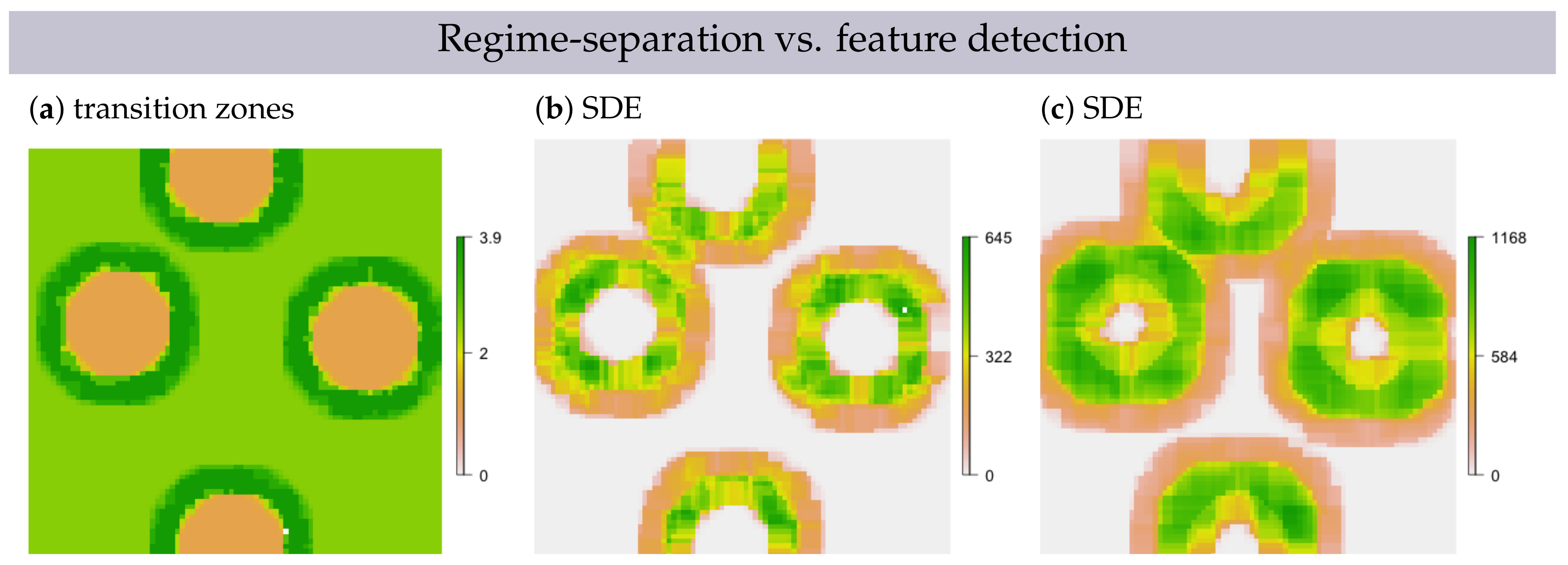
  • As outlined in Section 1, we expected to detect multi-scale features in the same places as scale-specific features, because all scale-specific features were found to originate from transition zones. However, the type of scale-specific features depends on the scale, which permits a hypothesis for the type of multi-scale features expected.
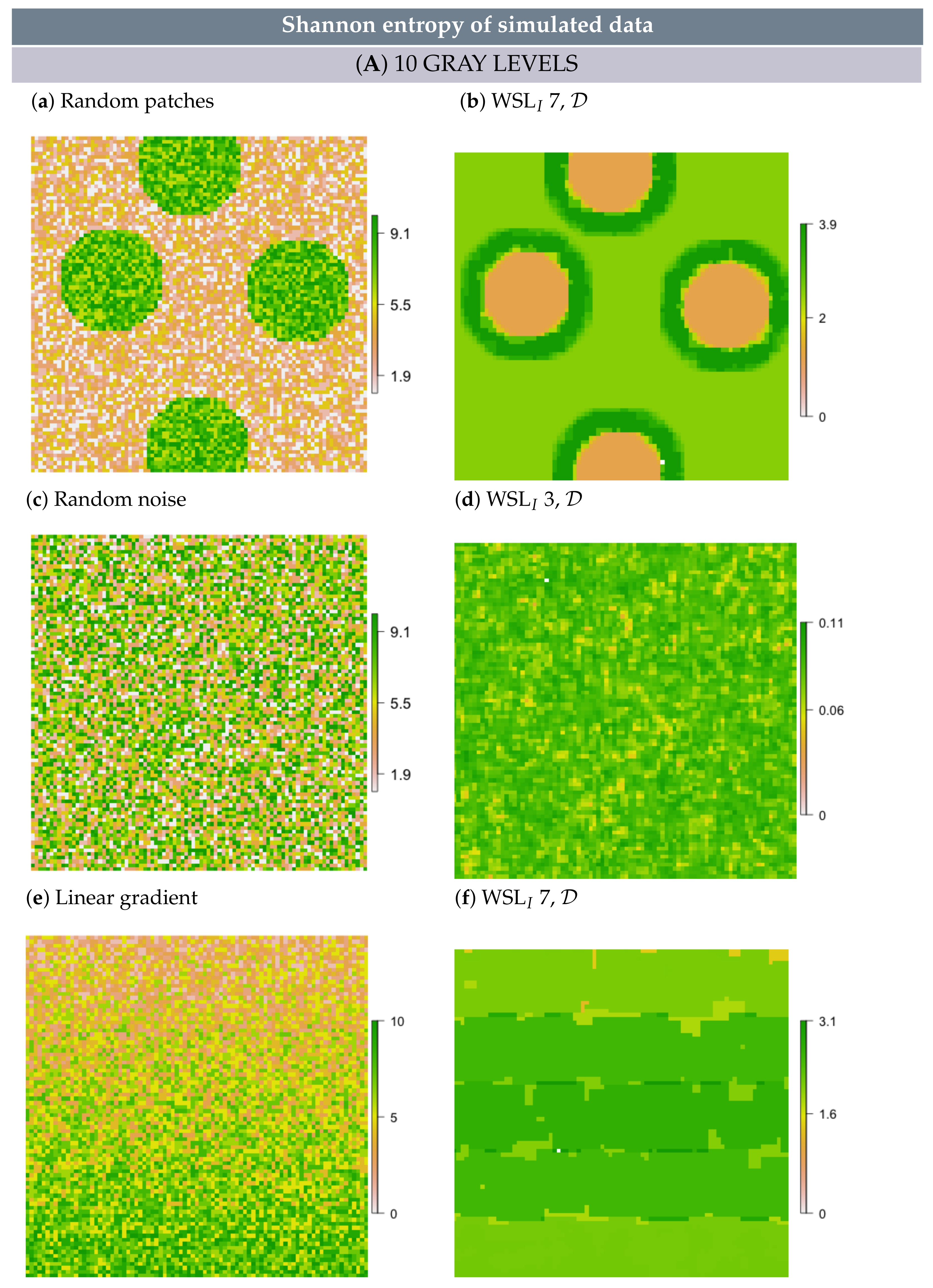
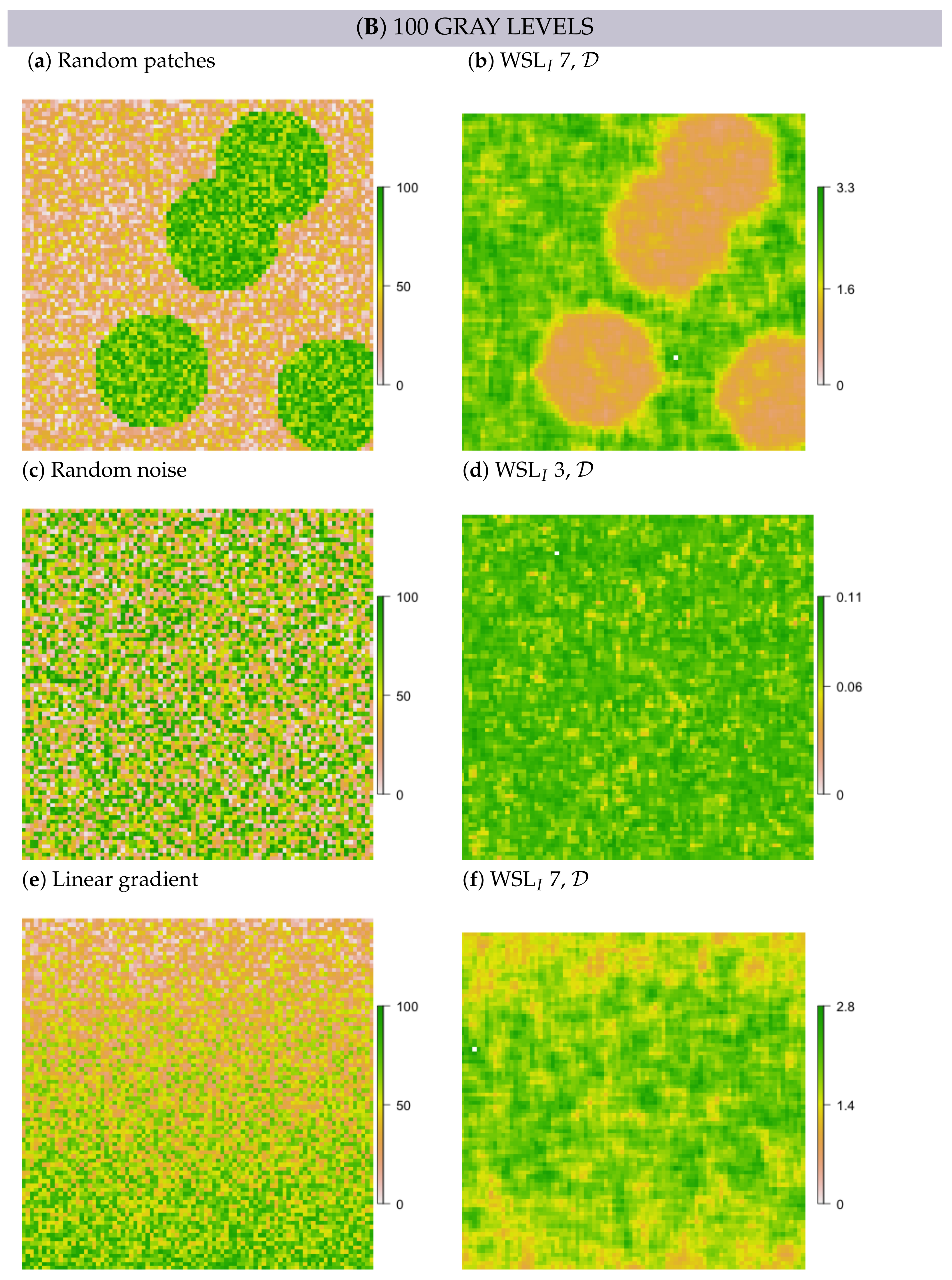
  • In simulated random patch data, we expected the edges between patches and the surrounding area to persevere as rings; hence, these rings would resemble multi-scale features.
  • In white noise and linear gradient data, we expected to detect no multi-scale features and also no scale-specific features, independent of metric formulation, scale and GL. However, some random structure may emerge, simply because values are not all the same.
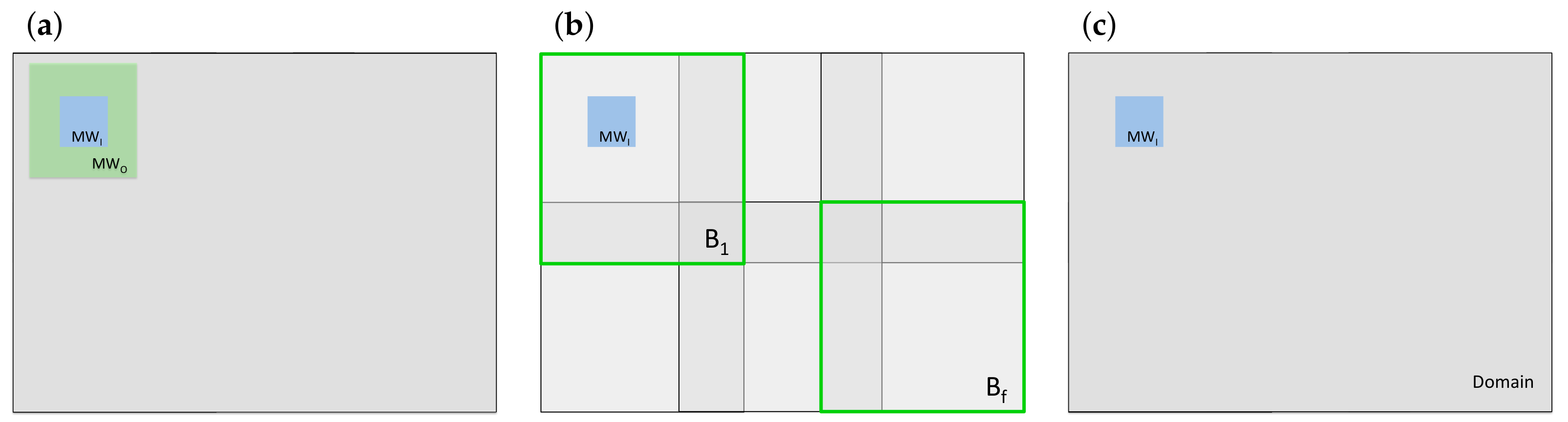
  • In the uni-scale approach, structural diversity is quantified based on all the information available on the considered scale. In the nested scales approach, prior information is only included about the value pairs that are present on the likelihood scale. This affects the structural diversity value assigned to the center pixel directly, because it is the sum of the individual metrics and hence is influenced by the number of elements that are summed up. We expected this to affect the smoothing of the structural diversity map. We further expected features to be contained to the inner scale and the size of features to be determined entirely by MW I , u .
  • When the inner and the outer scale are relatively similar in size, then k I approximates k O and n I approximates n O . This happens when double moving windows of similar size are employed. In this case, the depicted diverse structures are ‘produced’ by approximately equal amounts of information from the prior and from the likelihood. On the other hand, prior and likelihood will not differ that much, because inner and outer scale are of similar size and also because they are centered on the same pixel. Therefore, we expected to see similar features compared to the uni-scale approach and we expected the smoothing of scale-specific and of multi-scale features to be similar.
  • When the outer scale is much larger than the inner scale, then k O and n O dominate over k I and n I and will eventually be much larger because the number of pixel pairs increases rapidly with the WSL (Figure S3). An exception are cases where value pairs are very rare on the outer scale, but frequent on the inner scale. Yet, such rare cases may not be visible, because only one particular p i j p o s t might be affected. However when the prior dominates, then the spatial structure in the resulting map is mostly based on prior information. The larger the outer scale in relation to the inner scale, the stronger this relation will be. In such situations, the differences between features detected with and without prior information can be directly attributed to differences between the inner and the outer scale.
  • When the outer scale is the domain or a block, spatial structure is driven by k I , because k O , n O and n I are constant. Therefore, as the outer scale increases and the prior dominates the posterior, we expected diversity maps to eventually not differ anymore in terms of the types and sizes of features they depict.
    (a)
    When the outer scale is a block, we expected features to appear before a relatively homogeneous background inside each block, because in each block, the denominator is the same for every MW I , u and so is k O . Yet, we expected the different blocks to have slightly different background values, because k O is expected to be different in each block.
    (b)
    When the outer scale is D , we expected features to appear before a relatively homogeneous background in the whole structural diversity map, because the denominator and k O are the same for every MW I , u in the whole domain.

3. Results

The results reveal that combining information from different scales allows to detect multi-scale structural diversity features with certain method specifications. Some multi-scale features persist, while others emerge across scales (Figure 4). Multi-scale features populate the same places as scale-specific features, which supports Hypothesis 1. Additionally, the spatial regimes themselves (bareland and vegetation) can be detected, which will be referred to as regime-separation and further explained in Section 3.3. The size of the inner and outer extent affects the results, but feature detection is not improved by employing typical length-scales of structural diversity features. Further, GL dependency is affected by the use of prior information, as explained below. Structural diversity entropy is highest when no prior information is employed and lowest when the outer scale is the domain and this is the case for all data, all inner scales and alls GL and independent of δ . As the outer scale is increased, metric values decrease continuously and mild value fluctuations occur only in a few cases (Figure S11). Most structural diversity maps can be found in Supplementary Materials File S7. For better comparison, the color scale of all maps is set to a minimum of 0, which is the minimum value structural diversity entropy can take, independent of δ . We suggest that bounding lower metric values to 0 for display is generally advisable because otherwise small and large value differences may receive equal weights. Similarly, in cases where spatial structure is obscured by very high values, we display the 95% quantile. This reveals that the correspondent structure is detected by all method formulations, which in some cases reveals features and in other cases regime separation.

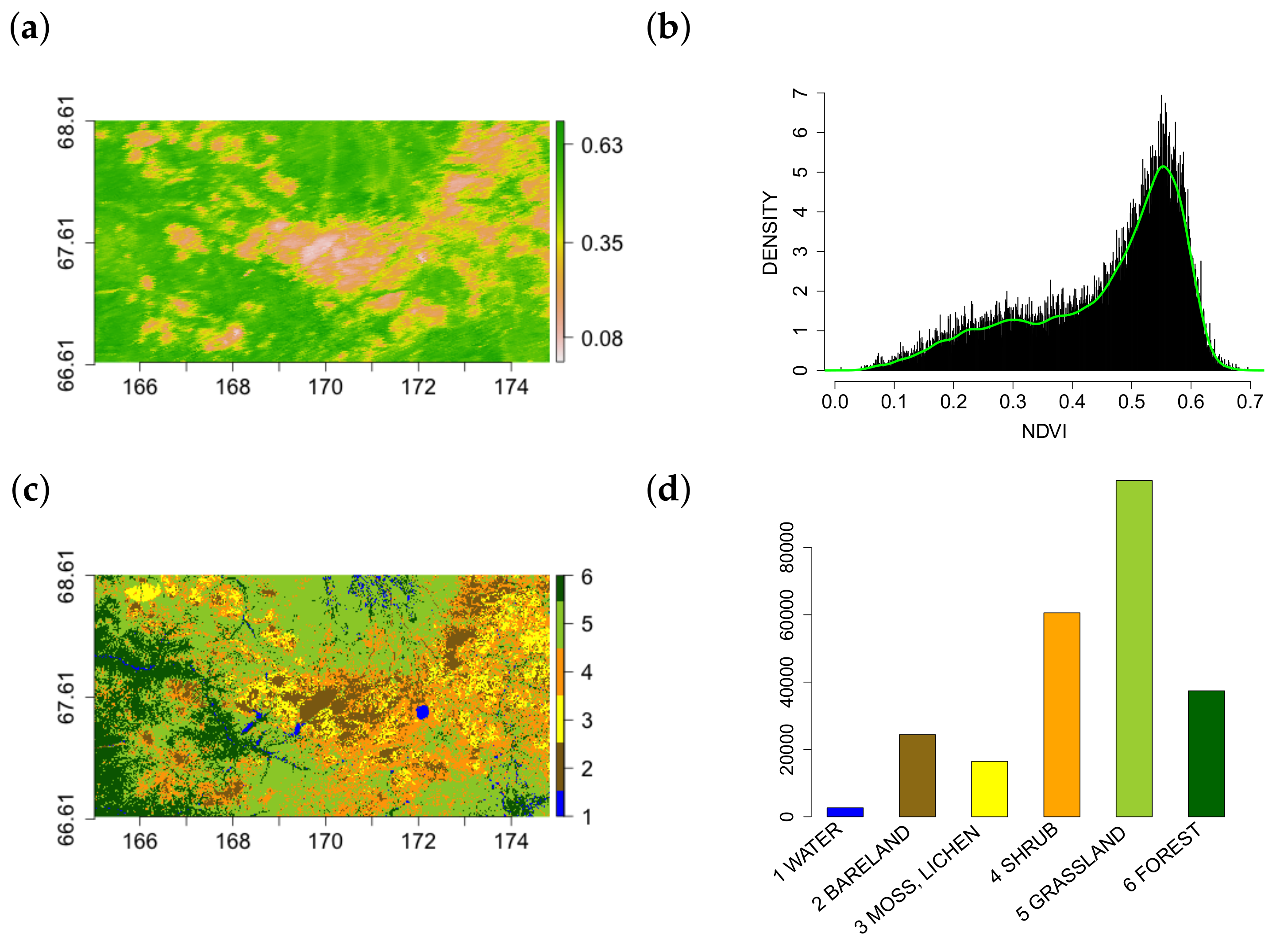
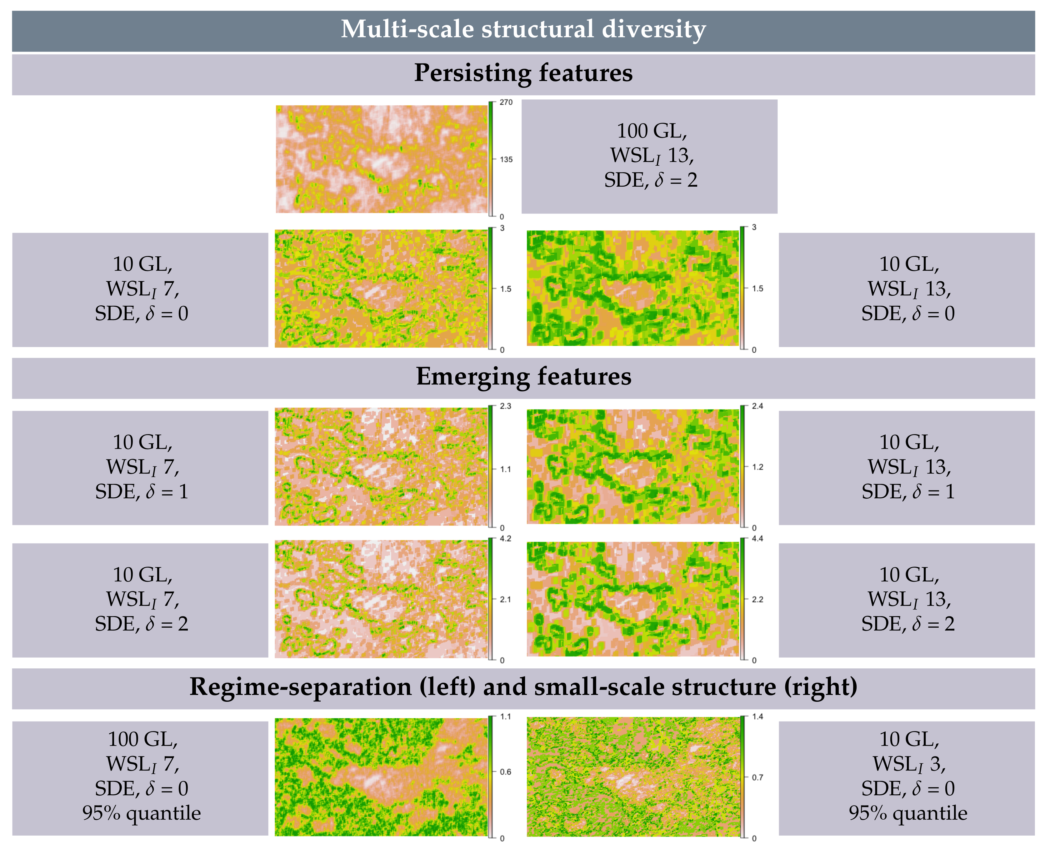
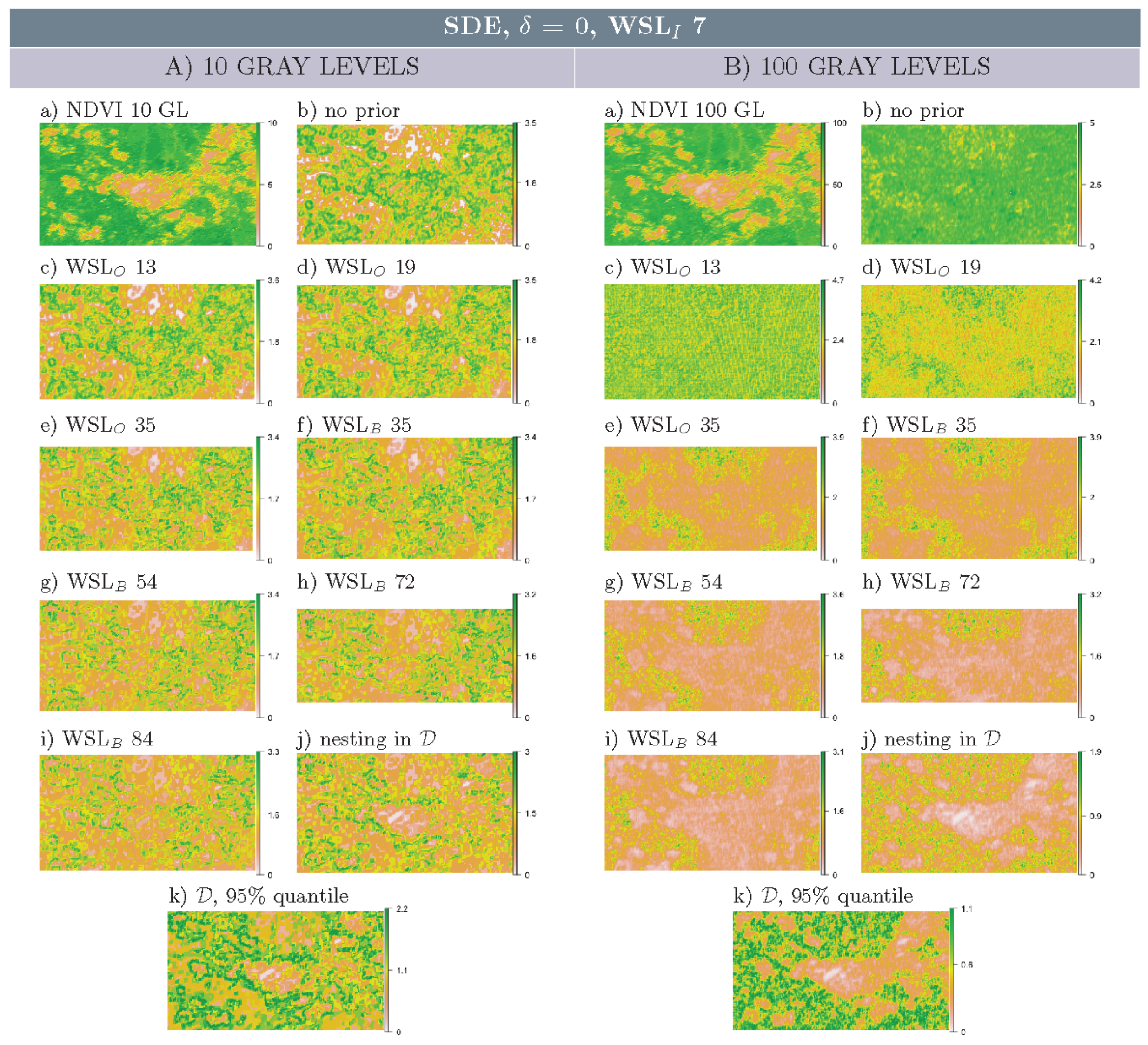
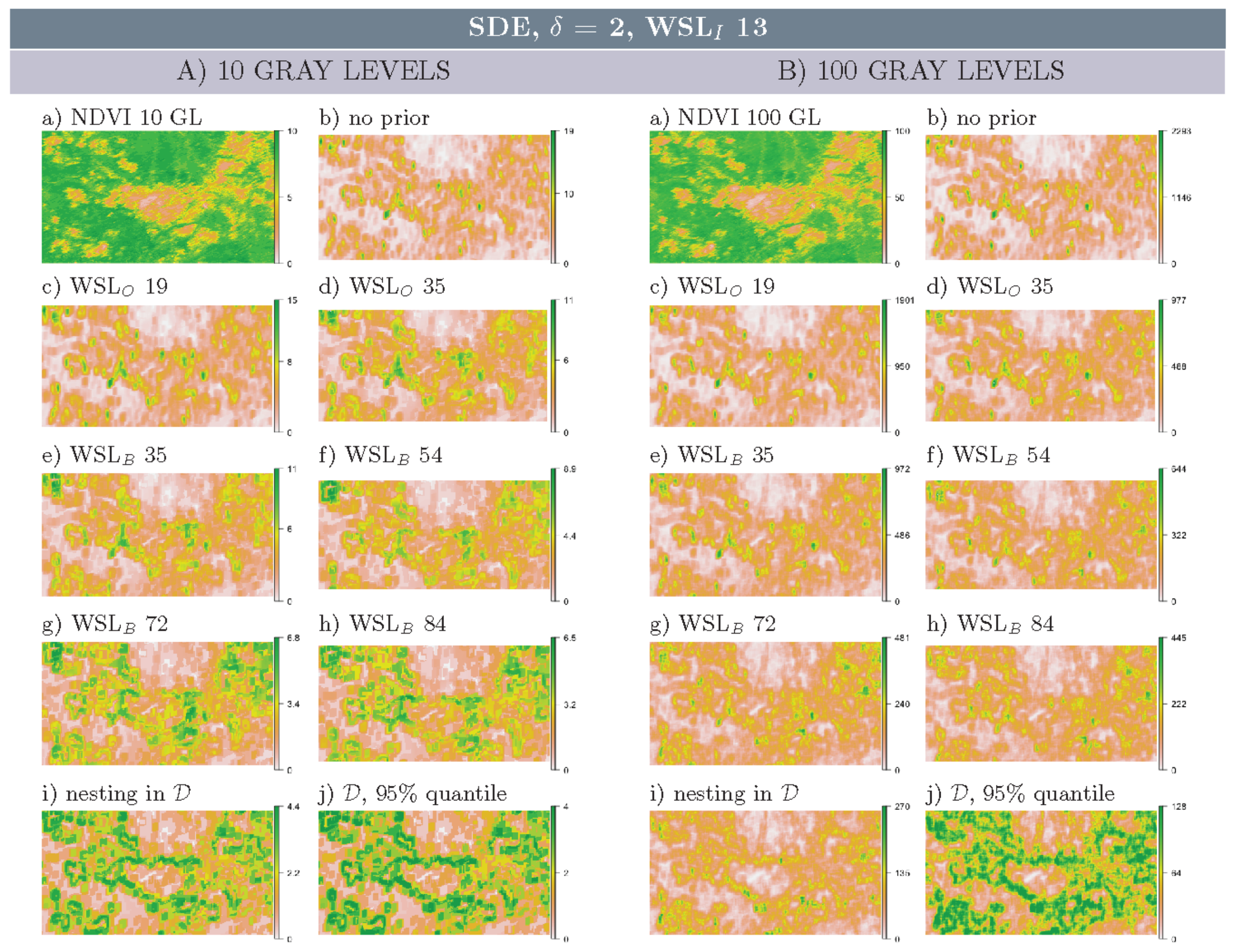
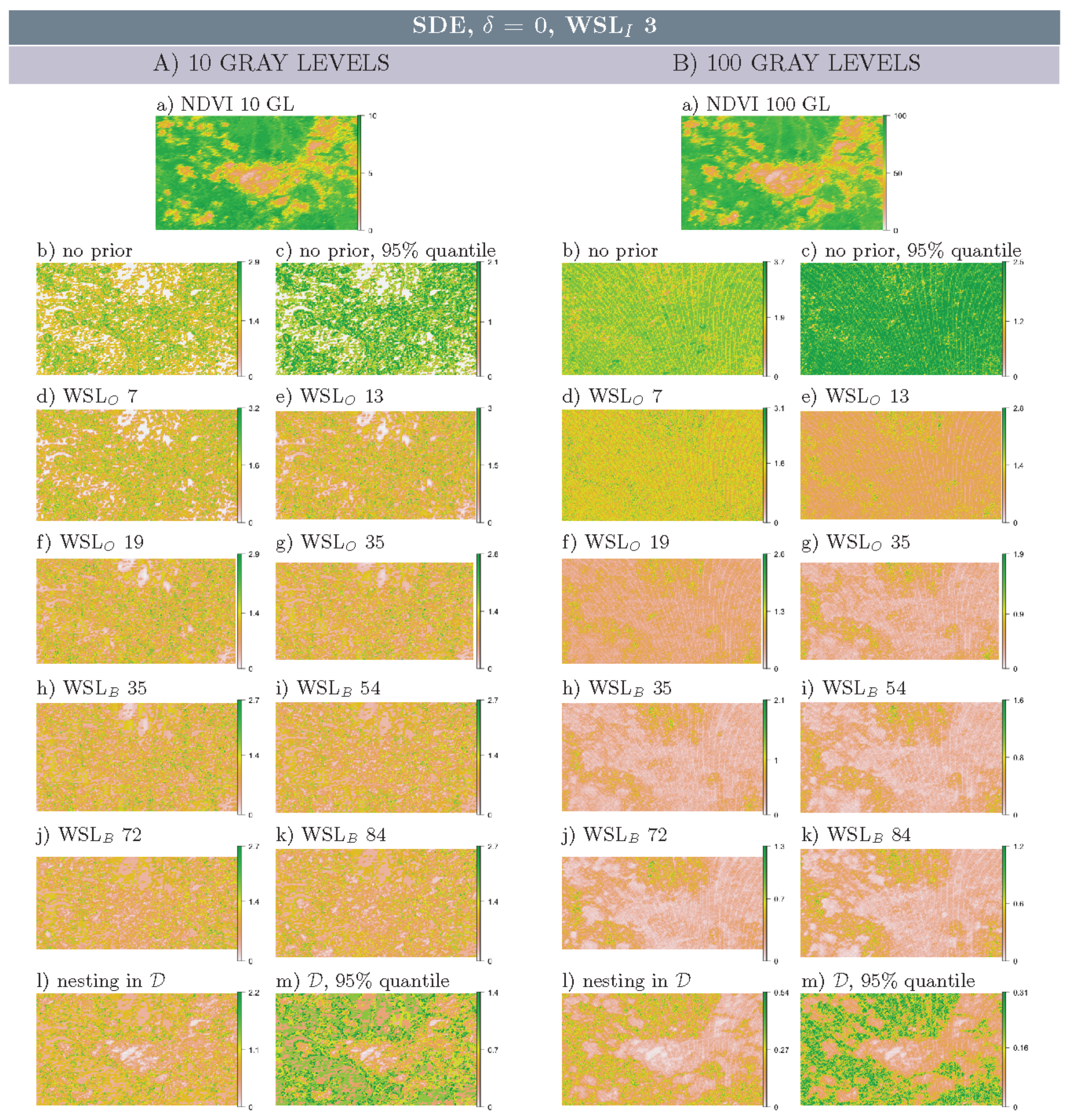
3.1. Multi-Scale Structural Diversity Features in NDVI Data

Multi-scale line features and patches are detected in NDVI data. Multi-scale line features resemble the transition zones between the bareland and the vegetation regime and multi-scale patch features originate from these transition zones (Figure 4). These results support Hypothesis 1. These features persist across scales or become apparent as the outer scale is increased. In all cases, they evolve to those features detected when the outer scale is the domain, supporting Hypothesis 7. Multi-scale line features are detected in data with 10 GLs, with inner scales of WSL I { 7 , 13 } and independent of δ (Figure 5A, Figure 6A, Figures S5A, S7A, S8A and S10A). Comparing multi-scale and scale-specific structural diversity maps reveals that multi-scale line features are scale-specific line features that persist across scales. However, these line features become narrower (i.e., more defined) when prior information is included and as the outer scale increases (Figure 5A and Figure S5A). The smoothing that is inevitable when larger moving windows are used to detect scale-specific line features disappears when prior information is included. This is in line with Hypothesis 4, where we expected smoothing to at least be affected.
In data with 10 GLs, scale-specific patch features morph into line features with both WSL { 7 , 13 } and independent of δ when prior information is included (Figure 6A, Figures S7A and S8A). In data with 100 GLs, the scale-specific patch features detected with WSL 13 and δ = 2 persist across scales and hence qualify as multi-scale structural diversity features (Figure 6B(b–i)). When δ = 1 , patches become less defined as the outer scale increases (in 100 GL data). This is particularly the case for WSL 7, but also for WSL 13 (Figures S7B and S8B).
To sum up, multi-scale line features are detected with inner scales of WSL { 7 , 13 } in data with 10 GLs and independent of δ , while multi-scale patch features are detected with WSL 13 in 100 GL data and with δ = 2 and to some extent with δ = 1 .

3.2. Multi-Scale Structural Diversity in Simulated Data

In simulated patch data, multi-scale structural diversity features are detected as rings (Figure 2A(b)), which supports Hypothesis 2. These features are detected with the same method specifications that reveal multi-scale features in NDVI data. Structural diversity quantified in 10 GL data with WSL I { 7 , 13 } reveals line features in NDVI data (for example, Figures S7A and S8A) and rings in random patch data (for example, Figures S12A and S13A), independent of δ . The findings suggest these to be ideal method specifications to detect multi-scale features. Structural diversity maps of simulated random noise data reveal either no or random structure, which supports Hypothesis 3 (Figure 2A,B(d)). Linear gradient data returns no or random structure in most cases, partly supporting Hypothesis 3 (Figure 2B(f)). However, when data has 10 GL and WSL I { 7 , 13 } , values are stratified into stripes, which is particularly pronounced with large outer scales (for example, Figure 2A(f)), Figures S33A and S34A).

3.3. Regime-Separation and GL-Dependency

When Shannon entropy is applied to data with 100 GLs without prior information, the scale-dependent maximum of the metric is responsible for structureless diversity maps. When prior information is included, structural diversity maps converge towards a situation where the two spatial regimes can be distinguished: The bareland regime by lower and the vegetation regime by higher entropy values (for example, Figure 5B, Figure 7B, Figures S6B and S7B). In other words, regime-separation is achieved when prior information is included, which reduces the GL-dependency of Shannon entropy. Regime-separation can also be observed in simulated random patch data where scale-specific rings morph into separate regimes (for example, Figure 2B(b), Figures S12B and S15B). Most of the time, the same method specifications reveal regime-separation in both NDVI and random patch data. Both data reveal regime-separation with δ { 0 , 1 } and independent of WSL I when data has 100 GLs.
Disagreement between structural diversity maps of NDVI and random patche data arises from (1) data with 10 GLs and inner scales of WSL I 3 and (2) data with 100 GLs and δ = 2 . When (1) WSL I 3 is applied to data with 10 GLs, random patch data depicts regime separation with all δ { 0 , 1 , 2 } (Figures S11, S14 and S17). In NDVI data, a mix of transition zones and regime separation appears, but is obstructed by small-scale structure and only visible within 95% quantiles. Separate regimes can be recognized with δ = 0 (Figure 7A) and narrow transition zones with δ { 1 , 2 } (Figures S6 and S9). In case (2), when δ = 2 , WSL I { 7 , 13 } and data has 100 GLs, patch data reveals rings that evolve to separate regimes (Figures S18 and S19). Yet, 95% quantiles of NDVI data reveal line features that appear almost identical to those multi-scale line features detected in data with 10 GLs (Figure 6B(j) and Figure S10B(k)). We suspected this disagreement to be influenced by the width of transition zones in NDVI vs. edges in patch data, which have virtually no width. We therefore tested patch data with wider edges, i.e., transition zones and we chose one of the structural diversity maps to do so. More specifically, we chose a map created with Shannon entropy in 10 GL random patch data, using WSL I 7. We binned these data to 100 GLs and calculated structural diversity entropy, using δ = 2 and WSL I { 7 , 13 } . The results depict rings, not regime separation (Figure 8). This means that these method specifications allow to distinguish between edges and transition zones.

3.4. Spatial Scale

Ideal inner scales to detect multi-scale structural diversity features are defined by WSL I { 7 , 13 } . The size of multi-scale features depends only on the size of the inner scale, which supports Hypothesis 4. Regime-separation and narrow line features can be detected on inner scales of WSL I 3, but the maps are obscured by small-scale structure in the latter case (Figure 7A,B(l,m)). While the sheer size of the outer scale affects the results, scales based on the effective range of structural diversity features does not improve feature detection. Using either the double moving window nesting scheme or the block nesting scheme, those outer scales that were chosen based on feature-typical length-scales lead to very similar results compared to scales that were chosen arbitrarily. Furthermore, differences between blocks and outer moving windows of the same size are minor, with structural diversity maps and metric values being the same or very similar (for example, Figure 5A,B(e,f)). Hypothesis 5 is supported because multi-scale and uni-scale structural diversity maps are most similar when inner and outer moving windows are of similar size (for example, Figure 5A(b,c)). As the outer scale increases, features either persist or emerge into what is depicted when the outer scale is the domain (NDVI data), supporting Hypothesis 7. When the outer scale is the domain, simulated patch features or the rings surrounding them are depicted before a relatively homogeneous background, as expected in Hypothesis 7b. In NDVI data, structure is visible in the background. When the outer scale is a block, structural diversity of simulated patch data reveals blocks in different colors in some cases and features appear before a relatively homogeneous background in each block, in line with Hypothesis 7a (Figures S12A(e), S13B(e), S15A(e) and S16B(e)). In NDVI data, blocks are never depicted in different background colors.
As the outer scale increases, ‘rectification’ can be observed in all structural diversity maps of data with 10 GLs and independent of δ when WSL I { 7 , 13 } are used. This means that line and ring features appear angular or cornered (for example, Figure 6A(g–i)). In random patch data, this can even occur with a uni-scale approach (Figure S19A). In random noise and linear gradient data, small rectangles appear (for example, Figures S27A and S30A).

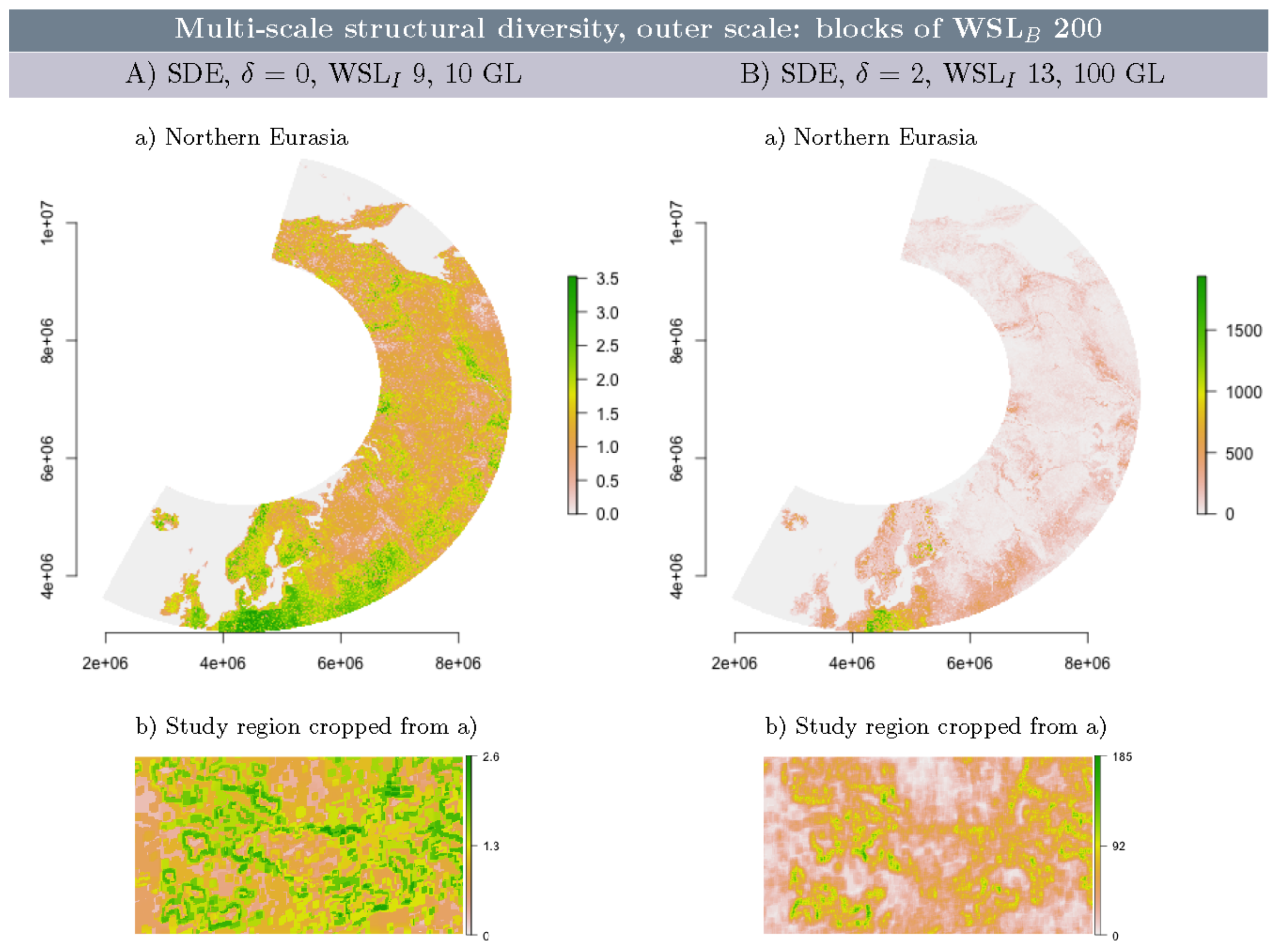
3.5. Multi-Scale Structural Diversity in Northern Eurasia

Structural diversity in northern Eurasia reveals large patterns, some appearing rather like lines, others more like patches or ‘areas’, such as high diversity in the whole of northern Europe. High structural diversity is detected in the same places with both method specifications. When the study region is ‘zoomed in’, structural diversity features are virtually identical to those detected when the method is applied directly to the study region. More specifically, the line features in Figure 9A(b) are similar to those in Figure 5A(j) and Figure S5A(i), which is reasonable since we used WSL I 9 in northern Eurasia and WSL I 7 and 13 in the study region. Patches in Figure 9B(b) are virtually identical to those in Figure 6B(i).

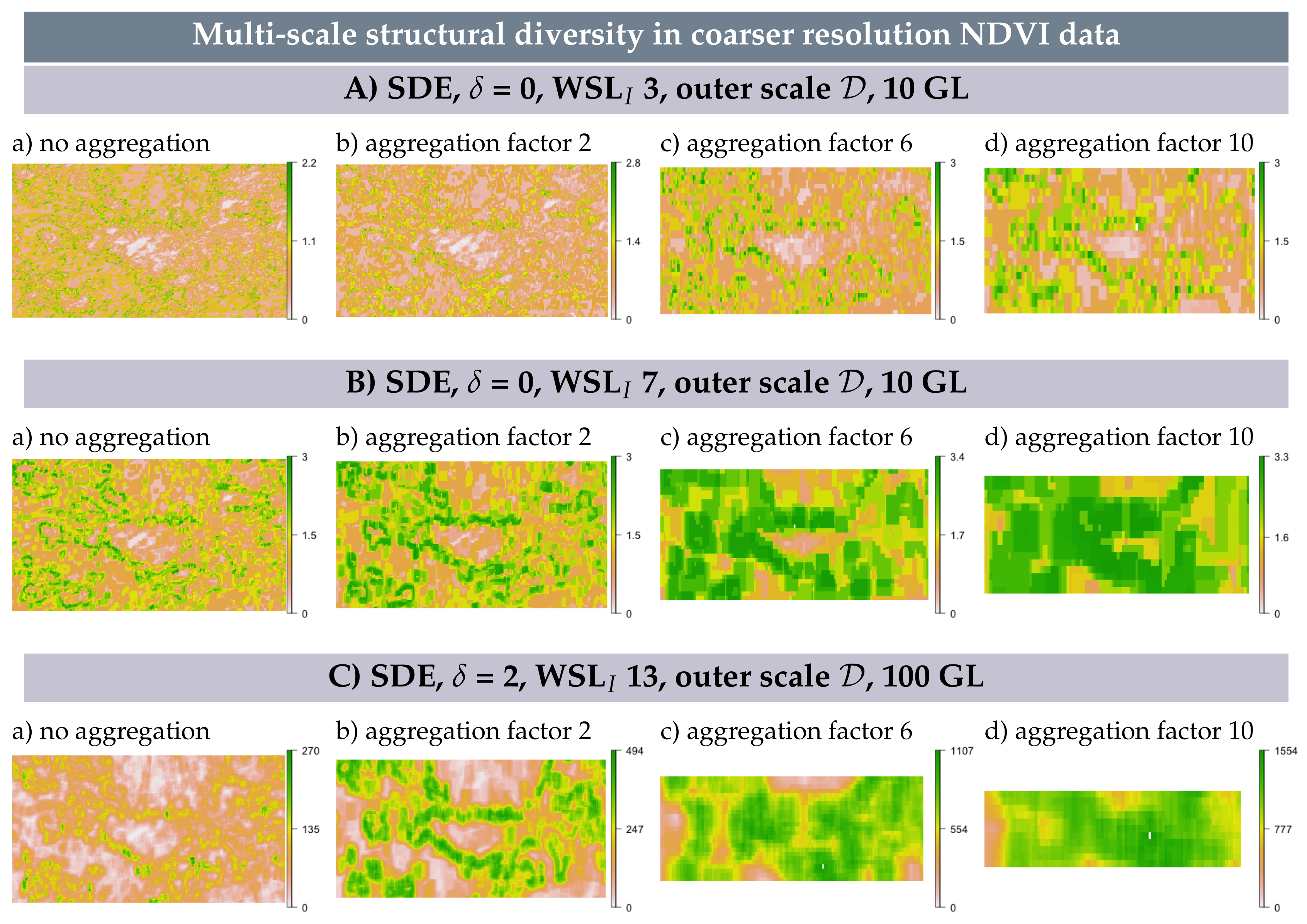
3.6. Multi-Scale Structural Diversity in Coarser Resolution NDVI Data

Figure 10 reveals the loss of information about structural diversity in the study region with increasing pixel size and the interaction between this information loss and the inner scale. On a local inner scale (WSL I 3), an aggregation factor of 2 leads to similar small-scale structures compared to the original resolution and aggregation factors 6 and 10 reveal structures that could be described as pixely and somewhat incomplete versions of the transition zones (Figure 10A).
On an inner scale of WSL I 7, an aggregation factor of 2 reveals similar line features compared to no aggregation. These features appear similar to those detected with WSL I 13 in the original resolution data. With aggregation factors 6 and 10, these line features are increasingly being fused to one large structure (Figure 10B).
On an inner scale of WSL I 13, aggregation of 2 × 2 pixels reveals that information about multi-scale patches is lost, but multi-scale line features are still detected. These line features appear similar to those detected in the original resolution data with the same method specifications when the 95% quantile is displayed. Aggregation factors of 6 and 10 reveal large, smooth structures (Figure 10C).

4. Discussion

One of the the main challenges in the study of landscape heterogeneity is the identification of significant structures that dominate across multiple spatial scales. Herein, we propose a novel method to combine information from different spatial scales with an empirical Bayesian model. This approach offers several advantages:
  • It can reveal the multi-scale character of landscape heterogeneity and detect multi-scale structural diversify features and spatial regimes. In particular, it can reveal near scale-invariant structures that are detected across almost all scales (such as line features in NDVI data).
  • The approach can be implemented without knowledge about typical length-scales of structural diversity features.
  • The smoothing effect inevitable in uni-scale moving window applications is removed.
  • Block and double moving window schemes can be used interchangeably, which allows the optimal choice from a computational perspective. The block nesting scheme is particularly suitable for processing very large datasets (such as NDVI in northern Eurasia).
The following interpretations are valid for the spatial configurations we tested in this study, which is direction-invariant co-occurrence of values in direct proximity. While some of the interpretations are naturally quite technical, we place our findings in an ecological context at the end of this section.

4.1. Multi-Scale Structural Diversity Features

Areas where structural diversity is found to be high on different spatial scales can reveal themselves as patches and line features. Such multi-scale structural diversity features can represent or emerge from transition zones between spatial regimes. This means that transition zones in NDVI data point to a change in landscape structure that alters vegetation productivity so dramatically that it can be detected across scales. Line features represent places of β structural diversity (spatial disorder) and multi-scale patches represent areas of high γ structural diversity (including the value gradient). Shannon entropy is also a measure of uncertainty [75], which means that transition zones are characterized by high uncertainty about landscape structure. In contrast, within spatial regimes, much information is redundant, in the sense that values could be interpolated if only a sample were available. Our results suggest that linear structural diversity features are quite robust against method specifications, while in high GL data, additional information manifests as patches (see Figure 4). The latter can be termed multi-scale hotspots, because they are detected with the largest exponent [28]. The role of structural diversity hotspots for other types of biodiversity hotspots is yet to be investigated. However, a positive association was recently established between potential hotspots of 3D structural complexity of forests and several high biodiversity ecoregions, suggesting further research may be worth while [85].

4.2. Spatial Scale

From a methods perspective, the smallest scale on which spatial structure can be quantified is the local scale (here defined by WSL 3), the domain can be interpreted as the global scale and intermediate scales can be called regional scales. Different behavior between local and regional scales has also been observed in other second-order texture metric applications, where regional scales were found to improve classification accurancy [79,86]. Yet, this issue is not method-specific, for example, fractal dimension, a measure of complexity, is also affected by unusual behavior on local scales [87]. Different behavior between local and regional scales is linked to the inseparable relation between resolution and extent, which also explains why ideal inner windows for feature detection can be identified. Pixel resolution represents the smallest resolvable scale and together, resolution and extent restrict the variability in the data and represent the scale of variation [80]. The scale of variation ultimately defines which landscape structures are resolved by the data. While both pixel size and extent affect the detection of landscape patterns [88,89,90], the former has been addressed more extensively and often under the umbrella terms ‘change of support’ [51,80] and ‘modifiable aerial unit problem’ [31]. The method presented herein requires no information about heterogeneity-typical scales; however, the resolution co-determines the scale on which structures are resolved. The results from Section 3.6 unveil that coarser resolution leads to a loss of information about spatial transition zones in the NDVI data of our study region. Hence, coarse resolution NDVI data are better suited for processes that manifest on larger scales (defined by both resolution and extent). In contrast, if the process under investigation manifests on smaller scales, finer resolution is necessary. Structural diversity metrics can then reveal landscape features that are not visible in coarser resolution data. Therefore, data resolution must be chosen with care, either based on process-typical scales or published research, or alternatively methods to assess the effect of resolution [31,51] can precede or be combined with the explicit treatment of extent [91].

4.3. Regime Separation

The inner scale restricts what size landscape structures can be detected, yet these structures are detected in relation to the outer scale. This explains why regime separation requires outer scales that are large enough to contain the regimes. The relative size of regimes differs, i.e., the bareland regime does not cover the same size area as the vegetation regime and likewise patches and the surrounding area are of different size. Therefore, k O differ between regimes. In patch data, k O are the same everywhere within patches and everywhere within the surrounding area, but distinctly different between them. The results suggest that in NDVI data, k O are similar everywhere within the bareland regime and within the vegetation regime, but, again, distinctly different between them.

4.4. Linear Gradient Stratification and Rectification

The removal of smoothing caused by moving windows comes at the expense of a smooth field when data has 10 GLs, revealed by rectification and stratification observed with WSL I { 7 , 13 } . This is due to the discrete character of 10 GL data and rectification is also attributable to the use of moving windows. In each moving window, k I compositions are unique and if the pixel pair arrangement differs strongly from a neighboring window, this is picked up by an abrupt change in structural diversity entropy values. Because square windows move in horizontal and vertical directions, these abrupt changes lead to rectification. In linear gradient data, stratification instead of rectification is visible because data are organized along a north–south gradient. Each row contains roughly the same number of different pixel values and the differences between v i and v j are roughly the same within each row. The same is true for columns, but between rows and columns, differences are distinct. This spatial organization is revealed as horizontal stripes and their width and position depends on the outer scale. Perfectly linear gradients on a perfectly placed grid are unlikely to occur in natural landscapes, although it may be possible to quantify the level of linearity in artificial landscapes.

4.5. Ecological Context and Possible Applications

Multi-scale structural diversity illuminates the hierarchical character of spatial heterogeneity and can delineate a landscape by its role for vegetation activity, energy and water balances. Interactions between soil, plants and atmosphere organize landscapes in regimes of spatially stable conditions, such as the bareland and the vegetation regimes in our study region. Such areas may often correlate with ecosystem types and both the regimes and the transition zones between them can now be localized. This enables automated monitoring of vegetation boundaries migrating uphill under warming temperatures [67], because such transition zones can be detected as delineated line or patch features. The block nesting scheme allows to detect multiple-scale landscape structure without smoothing effect on a continental scale. With the bare eye, one must zoom in to appreciate features detected in a sub-region of northern Eurasia like our study area, but it enables quantitative analyses of changes in landscape heterogeneity across scales. If structural diversity in northern Eurasia changes over time, it can indicate major ecosystem shifts related to some of the earth’s suggested tipping points [92]. This would have profound implications for processes from a micro- to a planetary level, ranging from microbial soil alterations to changes in the albedo and shifting climate patterns [13,93,94].
Multi-scale features so prominently define the structure of a landscape that it can be assumed they also play a crucial role for ecological and environmental processes on small and large scales [33]. What counts as small or large is defined by the scale of variation; however, the methods presented herein are invariant to pixel size in the sense that they operate identically, independent of resolution. With fine enough resolutions, these methods can likely detect rivers, cliffs, treelines and forest edges or hedgerows in agricultural areas. Applying these methods to continuous functional diversity maps could also shed light on the spatial component in the functioning of ecosystems, because it would reveal how traits such as nitrogen, chlorophyll, cartenoids, canopy height or leaf area, among others, are organized in space [95,96]. There are also many ways in which spatial scale is connected to animal abundance, composition and movement, be it through niche occupation, foraging behavior, dispersal range or based on landscape connectivity [97,98,99]. Rather than testing different size moving windows [98], it is now possible to specifically investigate the effect of the most dominant heterogeneity features, which comprise information from different scales.
Combining methods that adress the modifiable aerial unit problem with the methods presented in this study could enable the detection of borders of fragments and also of transition zones that are characterized by spatially disordered fragments. This may further illuminate how increasing fragmentation affects biodiversity and environmental functioning through processes interacting across multiple scales [100,101]. In this context, it is relevant that the largest exponent can reveal whether data comprises transition zones or abrupt edges, because the latter would be revealed as separate regimes when δ = 2 is applied to data with many GLs. However, gradual change is detected as line features or patches. Such information might be particularly useful for studying succession near edges resulting from forest logging, which affects biodiversity across taxa of flora and fauna [102,103]. In urban environments, edges have also been found some of the most influential structures for animal behavior [104] that can also demarcate breaks in the division of water and energy [105].
Further, the empirical Bayesian model used to realize a hierarchical concept of landscape heterogeneity is flexible enough to be extended to more spatial scales, temporal scales and to other thematic areas. This would target several interesting questions, for example, how information flow from the past to the present can improve our understanding of ecological and earth system processes, or the likelihood of observed structural diversity, considering how a landscape was structured in the past. The approach could be further advanced to become a model predicting future trajectories of structural diversity and potentially be adapted to include covariates in the process.

5. Conclusions

Structural diversity entropy meets the important challenge of quantifying landscape heterogeneity in continuous remote sensing data and contributes to a growing suite of methods that do not rely on the patch-mosaic paradigm [19,20]. The metric captures spatial disorder and value differences for a comprehensive measure of γ structural diversity. The empirical Bayesian model presented herein advances scale-specific structural diversity quantification with a direct model approach that integrates hierarchical levels of spatial scale. The approach reveals the multi-scale character of structural diversity by combining information from different scales. We applied this method to NDVI data in the northern high latitudes and we found that multi-scale structural diversity features, such as patches and line features, persist or become apparent across scales. Line features resemble the transition zones between spatial regimes and patches represent those areas within the transition zones where the value gradient is the steepest. Spatial regimes can also be distinguished based on their different structures when appropriate method specifications are applied. We developed three different schemes to nest smaller extents inside larger ones and we find the following associations: The smallest inner scale on which structural diversity can be quantified generally reveals additional small-scale structures, while larger inner scales are suitable for detecting multi-scale features. The outer scale need not be informed by typical length-scales, but its sheer size affects the results. We provide a roadmap that serves as a guide for the specification of structural diversity entropy, the choice of scales and GL reduction (summarized in File S1). The theoretical background described in this paper, along with the tools provided in the R package StrucDiv, allows for this method to be applied to other contexts. We hope that method and software will be a timely contribution to the numerous operating and soon-to-come satellite missions delivering ‘new information on physiological processes related to photosynthesis, transpiration and respiration and stress detection’ at a planetary level [18]. Our study advances information extraction from remote sensing imagery with an approach that holds the potential to reconsider scale in the characterization of environmental and biological landscape processes.

Supplementary Materials

The following supporting information can be downloaded at: https://0-www-mdpi-com.brum.beds.ac.uk/article/10.3390/rs15010014/s1.

Author Contributions

L.A.S. conceived the idea, developed the multi-scale approach, designed and carried out the experiment. R.F., M.J.S. and M.E.S. gave critical input to the experimental design. R.F. supervised the project. L.A.S. wrote the manuscript. All authors gave ciritcal feedback to the draft manuscript and have read and agreed to the published version of the manuscript.

Funding

This study was funded by the University Research Priority Program on Global Change and Biodiversity of the University of Zurich.

Data Availability Statement

All methods are accessible in the R package StrucDiv, which can be downloaded from the Comprehensive R Archive Network (CRAN) https://CRAN.R-project.org/package=StrucDiv, (accessed on 12 December 2022). NDVI data of the study region, simulated data and R scripts can be accesses from the Git repository https://git.math.uzh.ch/leilsc/multiScaleStrucDiv, (accessed on 12 December 2022). Vegetation index data of northern Eurasia can be accessed from https://0-doi-org.brum.beds.ac.uk/10.5281/zenodo.7401882, (accessed on 12 December 2022).

Conflicts of Interest

The authors declare no conflict to interest.

References

  1. Pielke, R.A.; Avissar, R. Influence of landscape structure on local and regional climate. Landsc. Ecol. 1990, 4, 133–155. [Google Scholar] [CrossRef]
  2. Lyford, M.E.; Jackson, S.T.; Betancourt, J.L.; Gray, S.T. Influence of landscape structure and climate variability on a late Holocene plant migration. Ecol. Monogr. 2003, 73, 567–583. [Google Scholar] [CrossRef]
  3. Torras, O.; Gil-Tena, A.; Saura, S. How does forest landscape structure explain tree species richness in a Mediterranean context? Biodivers. Conserv. 2008, 17, 1227–1240. [Google Scholar] [CrossRef]
  4. Walz, U.; Syrbe, R.U. Linking landscape structure and biodiversity. Ecol. Indic. 2013, 31, 1–5. [Google Scholar] [CrossRef]
  5. Stein, A.; Gerstner, K.; Kreft, H. Environmental heterogeneity as a universal driver of species richness across taxa, biomes and spatial scales. Ecol. Lett. 2014, 17, 866–880. [Google Scholar] [CrossRef] [PubMed]
  6. Noss, R.F. Indicators for Monitoring Biodiversity: A Hierarchical Approach. Conserv. Biol. 1990, 4, 355–364. [Google Scholar] [CrossRef]
  7. Estes, L.; Elsen, P.; Treuer, T.; Ahmed, L.; Caylor, K.; Chang, J.; Choi, J.; Ellis, E. The spatial and temporal domains of modern ecology. Nat. Ecol. Evol. 2018, 2, 819–826. [Google Scholar] [CrossRef] [Green Version]
  8. De Jong, R.; Verbesselt, J.; Zeileis, A.; Schaepman, M.E. Shifts in global vegetation activity trends. Remote Sens. 2013, 5, 1117–1133. [Google Scholar] [CrossRef] [Green Version]
  9. Guo, W.; Rees, W. Altitudinal forest-tundra ecotone categorization using texture-based classification. Remote Sens. Environ. 2019, 232, 111312. [Google Scholar] [CrossRef]
  10. ACIA. Impacts of a warming Arctic. In Arctic Climate Impact Assessment; Cambridge University Press: Cambridge, UK, 2005. [Google Scholar]
  11. IPCC. Climate Change 2007—The Physical Science Basis: Working Group I Contribution to the Fourth Assessment Report of the IPCC; Cambridge University Press: Cambridge, UK, 2007; Volume 4. [Google Scholar]
  12. Myers-Smith, I.; Elmendorf, S.; Beck, P.; Wilmking, M.; Hallinger, M.; Blok, D.; Tape, K.; Rayback, S.; Macias-Fauria, M.; Forbes, B.; et al. Climate sensitivity of shrub growth across the tundra biome. Nat. Clim. Chang. 2015, 5, 887–891. [Google Scholar] [CrossRef]
  13. Iturrate-Garcia, M.; O’Brien, M.J.; Khitun, O.; Abiven, S.; Niklaus, P.A.; Schaepman-Strub, G. Interactive effects between plant functional types and soil factors on tundra species diversity and community composition. Ecol. Evol. 2016, 6, 8126–8137. [Google Scholar] [CrossRef] [PubMed] [Green Version]
  14. Davidson, S.J.; Santos, M.J.; Sloan, V.L.; Reuss-Schmidt, K.; Phoenix, G.K.; Oechel, W.C.; Zona, D. Upscaling CH4 Fluxes Using High-Resolution Imagery in Arctic Tundra Ecosystems. Remote Sens. 2017, 9, 1227. [Google Scholar] [CrossRef] [Green Version]
  15. Montesano, P.M.; Neigh, C.S.R.; Macander, M.; Feng, M.; Noojipady, P. The bioclimatic extent and pattern of the cold edge of the boreal forest: The circumpolar taiga-tundra ecotone. Environ. Res. Lett. 2020, 15, 105019. [Google Scholar] [CrossRef]
  16. Kharuk, V.I.; Im, S.T.; Dvinskaya, M.L. Forest–tundra ecotone response to climate change in the Western Sayan Mountains, Siberia. Scand. J. For. Res. 2010, 25, 224–233. [Google Scholar] [CrossRef]
  17. Wilson, R.J.; Gutiérrez, D.; Gutiérrez, J.; Martínez, D.; Agudo, R.; Monserrat, V.J. Changes to the elevational limits and extent of species ranges associated with climate change. Ecol. Lett. 2005, 8, 1138–1146. [Google Scholar] [CrossRef]
  18. Ustin, S.L.; Middleton, E.M. Current and near-term advances in Earth observation for ecological applications. Ecol. Process. 2021, 10, 1–57. [Google Scholar] [CrossRef]
  19. McGarigal, K.; Tagil, S.; Cushman, S.A. Surface metrics: An alternative to patch metrics for the quantification of landscape structure. Landsc. Ecol. 2009, 24, 433–450. [Google Scholar] [CrossRef]
  20. Lausch, A.; Blaschke, T.; Haase, D.; Herzog, F.; Syrbe, R.U.; Tischendorf, L.; Walz, U. Understanding and quantifying landscape structure–A review on relevant process characteristics, data models and landscape metrics. Ecol. Model. 2015, 295, 31–41. [Google Scholar] [CrossRef]
  21. Lang, M.; Alleaume, S.; Luque, S.; Baghdadi, N.; Féret, J.B. Monitoring and Characterizing Heterogeneous Mediterranean Landscapes with Continuous Textural Indices Based on VHSR Imagery. Remote Sens. 2018, 10, 868. [Google Scholar] [CrossRef] [Green Version]
  22. Flury, R.; Gerber, F.; Schmid, B.; Furrer, R. Identification of dominant features in spatial data. Spat. Stat. 2021, 41, 100483. [Google Scholar] [CrossRef]
  23. Batty, M. Spatial entropy. Geogr. Anal. 1974, 6, 1–31. [Google Scholar] [CrossRef]
  24. Leibovici, D.G.; Claramunt, C.; Le Guyader, D.; Brosset, D. Local and global spatio-temporal entropy indices based on distance-ratios and co-occurrences distributions. Int. J. Geogr. Inf. Sci. 2014, 28, 1061–1084. [Google Scholar] [CrossRef] [Green Version]
  25. Altieri, L.; Cocchi, D.; Roli, G. A new approach to spatial entropy measures. Environ. Ecol. Stat. 2018, 25, 95–110. [Google Scholar] [CrossRef]
  26. Tukiainen, H.; Kiuttu, M.; Kalliola, R.; Alahuhta, J.; Hjort, J. Landforms contribute to plant biodiversity at alpha, beta and gamma levels. J. Biogeogr. 2019, 46, 1699–1710. [Google Scholar] [CrossRef] [Green Version]
  27. Izsák, J.; Papp, L. A link between ecological diversity indices and measures of biodiversity. Ecol. Model. 2000, 130, 151–156. [Google Scholar] [CrossRef]
  28. Schuh, L.; Santos, M.J.; Schaepman, M.; Furrer, R. Structural diversity entropy: A unified diversity measure to detect latent landscape features. Remote Sens. 2022. under review. [Google Scholar]
  29. Allen, C.R.; Holling, C.S. Cross-scale structure and scale breaks in ecosystems and other complex systems. Ecosystems 2002, 5, 315–318. [Google Scholar] [CrossRef]
  30. Wu, J.; Jelinski, D.E.; Luck, M.; Tueller, P.T. Multiscale analysis of landscape heterogeneity: Scale variance and pattern metrics. Geogr. Inf. Sci. 2000, 6, 6–19. [Google Scholar] [CrossRef] [PubMed] [Green Version]
  31. Hay, G.J.; Blaschke, T.; Marceau, D.J.; Bouchard, A. A comparison of three image-object methods for the multiscale analysis of landscape structure. ISPRS J. Photogramm. Remote Sens. 2003, 57, 327–345. [Google Scholar] [CrossRef]
  32. Fuhlendorf, S.D.; Woodward, A.J.; Leslie, D.M.; Shackford, J.S. Multi-scale effects of habitat loss and fragmentation on lesser prairie-chicken populations of the US Southern Great Plains. Landsc. Ecol. 2002, 17, 617–628. [Google Scholar] [CrossRef]
  33. Lyra-Jorge, M.C.; Ribeiro, M.C.; Ciocheti, G.; Tambosi, L.R.; Pivello, V.R. Influence of multi-scale landscape structure on the occurrence of carnivorous mammals in a human-modified savanna, Brazil. Eur. J. Wildl. Res. 2010, 56, 359–368. [Google Scholar] [CrossRef]
  34. Wiens, J.A. Spatial scaling in ecology. Funct. Ecol. 1989, 3, 385–397. [Google Scholar] [CrossRef]
  35. Levin, S.A. The Problem of Pattern and Scale in Ecology: The Robert H. MacArthur Award Lecture. Ecology 1992, 73, 1943–1967. [Google Scholar] [CrossRef]
  36. Sandel, B.; Smith, A.B. Scale as a lurking factor: Incorporating scale-dependence in experimental ecology. Oikos 2009, 118, 1284–1291. [Google Scholar] [CrossRef]
  37. O’Neill, R.V.; Gardner, R.H.; Milne, B.T.; Turner, M.G.; Jackson, B. Heterogeneity and spatial hierarchies. In Ecological Heterogeneity; Springer: Berlin, Germany, 1991; pp. 85–96. [Google Scholar] [CrossRef]
  38. Wheatley, M. Domains of scale in forest-landscape metrics: Implications for species-habitat modeling. Acta Oecol. 2010, 36, 259–267. [Google Scholar] [CrossRef]
  39. Geldenhuys, C.J. Bergwind Fires and the Location Pattern of Forest Patches in the Southern Cape Landscape, South Africa. J. Biogeogr. 1994, 21, 49–62. [Google Scholar] [CrossRef]
  40. Raffa, K.F.; Aukema, B.H.; Bentz, B.J.; Carroll, A.L.; Hicke, J.A.; Turner, M.G.; Romme, W.H. Cross-scale drivers of natural disturbances prone to anthropogenic amplification: The dynamics of bark beetle eruptions. Bioscience 2008, 58, 501–517. [Google Scholar] [CrossRef] [Green Version]
  41. Isbell, F.; Gonzalez, A.; Loreau, M.; Cowles, J.; Díaz, S.; Hector, A.; Mace, G.M.; Wardle, D.A.; O’Connor, M.I.; Duffy, J.E.; et al. Linking the influence and dependence of people on biodiversity across scales. Nature 2017, 546, 65–72. [Google Scholar] [CrossRef] [Green Version]
  42. Chust, G.; Pretus, J.; Ducrot, D.; Bedos, A.; Deharveng, L. Response of soil fauna to landscape heterogeneity: Determining optimal scales for biodiversity modeling. Conserv. Biol. 2003, 17, 1712–1723. [Google Scholar] [CrossRef]
  43. Geng, X.; Sun, K.; Ji, L.; Zhao, Y. A high-order statistical tensor based algorithm for anomaly detection in hyperspectral imagery. Sci. Rep. 2014, 4, 6869. [Google Scholar] [CrossRef]
  44. Zhao, C.; Wang, Y.; Qi, B.; Wang, J. Global and Local Real-Time Anomaly Detectors for Hyperspectral Remote Sensing Imagery. Remote Sens. 2015, 7, 3966–3985. [Google Scholar] [CrossRef] [Green Version]
  45. Moradi, S.; Moallem, P.; Sabahi, M.F. Fast and robust small infrared target detection using absolute directional mean difference algorithm. Signal Process. 2020, 177, 107727. [Google Scholar] [CrossRef]
  46. Hafiane, A.; Palaniappan, K.; Seetharaman, G. Joint adaptive median binary patterns for texture classification. Pattern Recognit. 2015, 48, 2609–2620. [Google Scholar] [CrossRef]
  47. Holmström, L.; Pasanen, L.; Furrer, R.; Sain, S.R. Scale space multiresolution analysis of random signals. Comput. Stat. Data Anal. 2011, 55, 2840–2855. [Google Scholar] [CrossRef]
  48. Krummel, J.; Gardner, R.; Sugihara, G.; O’neill, R.; Coleman, P. Landscape patterns in a disturbed environment. Oikos 1987, 48, 321–324. [Google Scholar] [CrossRef] [Green Version]
  49. Baatz, M. Multi resolution segmentation. In Beitraege zum AGIT-Symposium; Salzburg: Heidelberg, Germany, 2000; pp. 12–23. [Google Scholar]
  50. Stuber, E.F.; Gruber, L.F.; Fontaine, J.J. A Bayesian method for assessing multi-scale species-habitat relationships. Landsc. Ecol. 2017, 32, 2365–2381. [Google Scholar] [CrossRef]
  51. Wikle, C.K.; Berliner, L.M. Combining Information Across Spatial Scales. Technometrics 2005, 47, 80–91. [Google Scholar] [CrossRef]
  52. Robbins, H. An empirical Bayes approach to statistics. In Proceedings of the Third Berkeley Symposium on Mathematical Statistics and Probability, San Diego, CA, USA, 26–31 December 1954; Volume 1, pp. 157–163. [Google Scholar]
  53. Gotelli, N.J.; Ulrich, W. The empirical Bayes approach as a tool to identify non-random species associations. Oecologia 2010, 162, 463–477. [Google Scholar] [CrossRef]
  54. Krivoruchko, K.; Gribov, A. Evaluation of empirical Bayesian kriging. Spat. Stat. 2019, 32, 100368. [Google Scholar] [CrossRef]
  55. McCarthy, M.A. Bayesian Methods for Ecology; Cambridge University Press: Cambridge, UK, 2007. [Google Scholar]
  56. Casella, G. An introduction to empirical Bayes data analysis. Am. Stat. 1985, 39, 83–87. [Google Scholar]
  57. Carlin, B.P.; Louis, T.A. Empirical Bayes: Past, Present and Future. J. Am. Stat. Assoc. 2000, 95, 1286–1289. [Google Scholar] [CrossRef]
  58. Cowles, M.K.; Carlin, B.P. Markov chain Monte Carlo convergence diagnostics: A comparative review. J. Am. Stat. Assoc. 1996, 91, 883–904. [Google Scholar] [CrossRef]
  59. Hay, G.; Marceau, D.; Bouchard, A. Modeling multi-scale landscape structure within a hierarchical scale-space framework. Int. Arch. Photogramm. Remote. Sens. Spat. Inf. Sci. 2002, 34, 532–535. [Google Scholar]
  60. Baker, W.L. Spatially heterogeneous multi-scale response of landscapes to fire suppression. Oikos 1993, 66, 66–71. [Google Scholar] [CrossRef]
  61. Lindeberg, T.; Haar Romeny, B.M.t. Linear scale-space I: Basic theory. In Geometry-Driven Diffusion in Computer Vision; Springer: Berlin, Germany, 1994; pp. 1–38. [Google Scholar]
  62. De Jong, R.; Schaepman, M.E.; Furrer, R.; De Bruin, S.; Verburg, P.H. Spatial relationship between climatologies and changes in global vegetation activity. Glob. Chang. Biol. 2013, 19, 1953–1964. [Google Scholar] [CrossRef] [PubMed]
  63. Guay, K.C.; Beck, P.S.; Berner, L.T.; Goetz, S.J.; Baccini, A.; Buermann, W. Vegetation productivity patterns at high northern latitudes: A multi-sensor satellite data assessment. Glob. Chang. Biol. 2014, 20, 3147–3158. [Google Scholar] [CrossRef] [Green Version]
  64. Schuh, L.; Schaepman, M.; Santos, M.J.; de Jong, R.; Furrer, R. Advancing Texture Metrics to Model Landscape Heterogeneity. In Proceedings of the IGARSS 2020—2020 IEEE International Geoscience and Remote Sensing Symposium, Waikoloa, HI, USA, 26 September–2 October 2020; pp. 2735–2738. [Google Scholar] [CrossRef]
  65. Rahbek, C. The role of spatial scale and the perception of large-scale species-richness patterns. Ecol. Lett. 2005, 8, 224–239. [Google Scholar] [CrossRef]
  66. Whittaker, R.H. Communities and Ecosystems; Macmillan: New York, NY, USA, 1970. [Google Scholar]
  67. Sundstrom, S.M.; Eason, T.; Nelson, R.J.; Angeler, D.G.; Barichievy, C.; Garmestani, A.S.; Graham, N.A.; Granholm, D.; Gunderson, L.; Knutson, M.; et al. Detecting spatial regimes in ecosystems. Ecol. Lett. 2017, 20, 19–32. [Google Scholar] [CrossRef] [Green Version]
  68. Didan, K. MOD13Q1 Dataset. MODIS Terra Vegetation Indices 16-Day L3 Global 250m SIN Grid V006. NASA EOSDIS Land Processes DAAC. 2015. Available online: https://lpdaac.usgs.gov/products/mod13q1v006/ (accessed on 12 December 2022).
  69. Gorelick, N.; Hancher, M.; Dixon, M.; Ilyushchenko, S.; Thau, D.; Moore, R. Google Earth Engine: Planetary-scale geospatial analysis for everyone. Remote. Sens. Environ. 2017, 202, 18–27. [Google Scholar] [CrossRef]
  70. R Core Team. R: A Language and Environment for Statistical Computing. 2022. Available online: https://intro2r.com/citing-r.html (accessed on 12 December 2022).
  71. Hijmans, R.J. Raster: Geographic Data Analysis and Modeling. R Package Version 2.9-5. 2019. Available online: https://cran.r-project.org/web/packages/raster/raster.pdf (accessed on 12 December 2022).
  72. Furrer, R.; Sain, S.R. spam: A Sparse Matrix R Package with Emphasis on MCMC Methods for Gaussian Markov Random Fields. J. Stat. Softw. 2010, 36, 1–25. [Google Scholar] [CrossRef] [Green Version]
  73. Nychka, D.; Furrer, R.; Paige, J.; Sain, S. Fields: Tools for Spatial Data. R Package Version 13.3. 2021. Available online: https://dnychka.github.io/portfolio/fields/ (accessed on 12 December 2022).
  74. Schuh, L.; Furrer, R. StrucDiv: Spatial Structural Diversity Quantification in Raster Data. 2022. Available online: https://cran.r-project.org/web/packages/StrucDiv/StrucDiv.pdf (accessed on 12 December 2022).
  75. Shannon, C.E. A mathematical theory of communication. Bell Syst. Tech. J. 1948, 27, 379–423. [Google Scholar] [CrossRef]
  76. O’Neill, R.V.; Krummel, J.; Gardner, R.e.a.; Sugihara, G.; Jackson, B.; DeAngelis, D.; Milne, B.; Turner, M.G.; Zygmunt, B.; Christensen, S.; et al. Indices of landscape pattern. Landsc. Ecol. 1988, 1, 153–162. [Google Scholar] [CrossRef]
  77. Haralick, R.M.; Shanmugam, K.; Dinstein, I. Textural Features for Image Classification. IEEE Trans. Syst. Man Cybern. 1973, SMC-3, 610–621. [Google Scholar] [CrossRef] [Green Version]
  78. Gonzalez, R.C.; Woods, R.E. Digital Image Processing; Prentice Hall: Upper Saddle River, NJ, USA, 2008. [Google Scholar]
  79. Clausi, D.A. An analysis of co-occurrence texture statistics as a function of grey level quantization. Can. J. Remote Sens. 2002, 28, 45–62. [Google Scholar] [CrossRef]
  80. Cressie, N.A. Statistics for Spatial Data; John Wiley and Sons Inc.: New York, NY, USA, 1993. [Google Scholar]
  81. Gelman, A.; Carlin, J.B.; Stern, H.S.; Rubin, D.B. Bayesian Data Analysis, 2nd ed.; Chapman & Hall/CRC: Boca Raton, FL, USA, 2004. [Google Scholar]
  82. Navarro, D.; Perfors, A. An Introduction to the Beta-Binomial Model; University of Adelaide: Adelaide, Australia, 2005. [Google Scholar]
  83. Jeffreys, H.; Jeffreys, B.; Swirles, B. Methods of Mathematical Physics; Cambridge University Press: Cambridge, UK, 1999. [Google Scholar]
  84. Weisstein, E.W. Beta Function. 2002. Available online: https://mathworld.wolfram.com/ (accessed on 12 December 2022).
  85. Ehbrecht, M.; Seidel, D.; Annighöfer, P.; Kreft, H.; Köhler, M.; Zemp, D.C.; Puettmann, K.; Nilus, R.; Babweteera, F.; Willim, K.; et al. Global patterns and climatic controls of forest structural complexity. Nat. Commun. 2021, 12, 519. [Google Scholar] [CrossRef] [PubMed]
  86. Guo, W.; Rees, G.; Hofgaard, A. Delineation of the forest-tundra ecotone using texture-based classification of satellite imagery. Int. J. Remote Sens. 2020, 41, 6384–6408. [Google Scholar] [CrossRef]
  87. Loke, L.H.; Chisholm, R.A. Measuring habitat complexity and spatial heterogeneity in ecology. Ecol. Lett. 2022, 25, 2269–2288. [Google Scholar] [CrossRef]
  88. Turner, M.G.; O’Neill, R.V.; Gardner, R.H.; Milne, B.T. Effects of changing spatial scale on the analysis of landscape pattern. Landsc. Ecol. 1989, 3, 153–162. [Google Scholar] [CrossRef]
  89. Schneider, D.C. The rise of the concept of scale in ecology: The concept of scale is evolving from verbal expression to quantitative expression. BioScience 2001, 51, 545–553. [Google Scholar] [CrossRef] [Green Version]
  90. Wu, J. Effects of changing scale on landscape pattern analysis: Scaling relations. Landsc. Ecol. 2004, 19, 125–138. [Google Scholar] [CrossRef]
  91. Marceau, D.; Hay, G. Remote Sensing Contributions to the Scale Issue. Can. J. Remote Sens. 1999, 25, 357–366. [Google Scholar] [CrossRef]
  92. Lenton, T.; Rockström, J.; Gaffney, O.; Rahmstorf, S.; Richardson, K.; Steffen, W.; Schellnhuber, H. Climate tipping points—Too risky to bet against. Nature 2019, 575, 592–595. [Google Scholar] [CrossRef] [PubMed] [Green Version]
  93. Gauthier, S.; Bernier, P.; Kuuluvainen, T.; Shvidenko, A.Z.; Schepaschenko, D.G. Boreal forest health and global change. Science 2015, 349, 819–822. [Google Scholar] [CrossRef] [PubMed]
  94. Davidson, S.J.; Santos, M.J.; Sloan, V.L.; Watts, J.D.; Phoenix, G.K.; Oechel, W.C.; Zona, D. Mapping Arctic Tundra Vegetation Communities Using Field Spectroscopy and Multispectral Satellite Data in North Alaska, USA. Remote Sens. 2016, 8, 978. [Google Scholar] [CrossRef] [Green Version]
  95. Jetz, W.; Cavender-Bares, J.; Pavlick, R.; Schimel, D.; Davis, F.W.; Asner, G.P.; Guralnick, R.; Kattge, J.; Latimer, A.M.; Moorcroft, P.; et al. Monitoring plant functional diversity from space. Nat. Plants 2016, 2, 1–5. [Google Scholar] [CrossRef] [Green Version]
  96. Schneider, F.D.; Morsdorf, F.; Schmid, B.; Petchey, O.L.; Hueni, A.; Schimel, D.S.; Schaepman, M.E. Mapping functional diversity from remotely sensed morphological and physiological forest traits. Nat. Commun. 2017, 8, 1441. [Google Scholar] [CrossRef] [Green Version]
  97. Abdel Moniem, H.E.M.; Holland, J.D. Habitat connectivity for pollinator beetles using surface metrics. Landsc. Ecol. 2013, 28, 1251–1267. [Google Scholar] [CrossRef]
  98. Holland, J.D.; Yang, S. Multi-scale studies and the ecological neighborhood. Curr. Landsc. Ecol. Rep. 2016, 1, 135–145. [Google Scholar] [CrossRef] [Green Version]
  99. Rodríguez-Gómez, G.B.; Villaseñor, N.R.; Orellana, J.I.; Pozo, R.A.; Fontúrbel, F.E. A multi-scale assessment of habitat disturbance on forest animal abundance in South American temperate rainforests. For. Ecol. Manag. 2022, 520, 120360. [Google Scholar] [CrossRef]
  100. Liu, J.; Wilson, M.; Hu, G.; Liu, J.; Wu, J.; Yu, M. How does habitat fragmentation affect the biodiversity and ecosystem functioning relationship? Landsc. Ecol. 2018, 33, 341–352. [Google Scholar] [CrossRef]
  101. Rocchini, D.; Bacaro, G.; Chirici, G.; Da Re, D.; Feilhauer, H.; Foody, G.M.; Galluzzi, M.; Garzon-Lopez, C.X.; Gillespie, T.W.; He, K.S.; et al. Remotely sensed spatial heterogeneity as an exploratory tool for taxonomic and functional diversity study. Ecol. Indic. 2018, 85, 983–990. [Google Scholar] [CrossRef]
  102. Meiners, S.J. Multiple Effects of the Forest Edge on the Structure of an Old Field Plant Community; Rutgers, The State University of New Jersey: New Brunswick, NJ, USA, 1999. [Google Scholar]
  103. Wirth, R.; Meyer, S.T.; Leal, I.R.; Tabarelli, M. Plant herbivore interactions at the forest edge. In Progress in Botany; Springer: Berlin, Germany, 2008; pp. 423–448. [Google Scholar]
  104. Brearley, G.; McAlpine, C.; Bell, S.; Bradley, A. Influence of urban edges on stress in an arboreal mammal: A case study of squirrel gliders in southeast Queensland, Australia. Landsc. Ecol. 2012, 27, 1407–1419. [Google Scholar] [CrossRef]
  105. Cohard, J.M.; Rosant, J.M.; Rodriguez, F.; Andrieu, H.; Mestayer, P.G.; Guillevic, P. Energy and water budgets of asphalt concrete pavement under simulated rain events. Urban Clim. 2018, 24, 675–691. [Google Scholar] [CrossRef]
Figure 1. (a) Average NDVI of the growing season 2018 in the study region, (b) NDVI histogram with superimposed density estimate, (c) categorical land cover of the study region, (d) barplot of LCCs. Adapted from [28].
Remotesensing 15 00014 g001
Figure 2. Simulated data: (A,B) (a) random patches, (c) random noise, (e) linear gradient data. Structural diversity of (b) random patches, (d) random noise, (f) linear gradient data. The outer scale is the domain, D , in all cases, the inner scale is defined by WSL I . Structural diversity entropy with δ = 0 was employed in all cases.
Remotesensing 15 00014 g002aRemotesensing 15 00014 g002b
Figure 3. Three nesting schemes, (a) inner moving window MW I , u nested inside outer moving window MW O , u , (b) MW I , u nested inside blocks B e , and (c) MW I , u nested inside the domain.
Remotesensing 15 00014 g003
Figure 4. Structural diversity entropy (SDE), quantified wit δ { 0 , 1 , 2 } , the outer scale is D in all cases. Minimum values displayed are set to 0.
Remotesensing 15 00014 g004
Figure 5. Structural diversity entropy (SDE), δ = 0, WSL I 7. Minimum values displayed are set to 0. (A,B(k)) Nesting in D , 95% quantiles.
Remotesensing 15 00014 g005
Figure 6. Structural diversity entropy (SDE), δ = 2, WSL I 13. Minimum values displayed are set to 0. (A,B(j)) Nesting in D , 95% quantiles.
Remotesensing 15 00014 g006
Figure 7. Structural diversity entropy (SDE), δ = 0, WSL I 3. Minimum values displayed are set to 0. (A,B(c)) No nesting, 95% quantiles, (A,B(m)) Nesting in D , 95% quantiles.
Remotesensing 15 00014 g007
Figure 8. (a) Random patches surrounded by transition zones, (b) structural diversity entropy (SDE), δ = 2 , inner scale WSL I 7, outer scale D , (c) SDE, δ = 2 , inner scale WSL I 13, outer scale D .
Remotesensing 15 00014 g008
Figure 9. Structural diversity entropy (SDE), (a) of northern Eurasia, (b) of the study region, which was cropped from northern Eurasia.
Remotesensing 15 00014 g009
Figure 10. Structural diversity entropy (SDE), quantified wit δ { 0 , 2 } , the outer scale is D in all cases. Minimum values displayed are set to 0.
Remotesensing 15 00014 g010
Disclaimer/Publisher’s Note: The statements, opinions and data contained in all publications are solely those of the individual author(s) and contributor(s) and not of MDPI and/or the editor(s). MDPI and/or the editor(s) disclaim responsibility for any injury to people or property resulting from any ideas, methods, instructions or products referred to in the content.

