Object Counting in Remote Sensing via Triple Attention and Scale-Aware Network

Abstract

Object counting is a fundamental task in remote sensing analysis. Nevertheless, it has been barely studied compared with object counting in natural images due to the challenging factors, e.g., background clutter and scale variation. This paper proposes a triple attention and scale-aware network (TASNet). Specifically, a triple view attention (TVA) module is adopted to remedy the background clutter, which executes three-dimension attention operations on the input tensor. In this case, it can capture the interaction dependencies between three dimensions to distinguish the object region. Meanwhile, a pyramid feature aggregation (PFA) module is employed to relieve the scale variation. The PFA module is built in a four-branch architecture, and each branch has a similar structure composed of dilated convolution layers to enlarge the receptive field. Furthermore, a scale transmit connection is introduced to enable the lower branch to acquire the upper branch’s scale, increasing the output’s scale diversity. Experimental results on remote sensing datasets prove that the proposed model can address the issues of background clutter and scale variation. Moreover, it outperforms the state-of-the-art (SOTA) competitors subjectively and objectively.

1. Introduction

With the rapid development of remote sensing technologies and satellite platforms, high-quality and quantity remote sensing images are provided for implementing specific tasks, e.g., object detection [1,2], image classification [3] and image super-resolution [4]. Compared with the aforementioned tasks which have been extensively investigated, object counting in remote sensing images has been barely explored due to the challenging factors, e.g., background clutter and scale variation.

The purpose of object counting is to infer the number of instances existing in images. It plays an essential and fundamental role in urban planning [5], environment management [6], monitoring system [7] and public safety [8]. Object counting has drawn much attention, and various approaches have been proposed which can be classified in three categories, i.e., detection-based methods [9,10], regression-based methods [11] and density estimation-based methods [12,13]. The detection-based methods generate bounding boxes by a designed object detector, and they sum the bounding boxes to obtain the object counts. These methods are suitable for counting large objects in sparse scenes. Once the scene becomes crowded and the object size is small, the counting performance will deteriorate dramatically. To address this issue, the regression-based methods are proposed to directly learn a mapping from the image to counts. They can deal with the problem of occlusion and complex background while ignoring the spatial information. Nowadays, benefiting from the strong feature representation ability of convolutional neural network (CNN), density estimation-based methods have outperformed the aforementioned two methods and become the mainstream in the domain of object counting [14]. The key idea of the density estimation-based method is to regress a density map by a CNN, and then, the pixels of the map are summed to generate the final count value [14,15,16]. Nevertheless, the scale variation and background clutter still constrain the accuracy and robustness of the object counting, especially in remote sensing images.

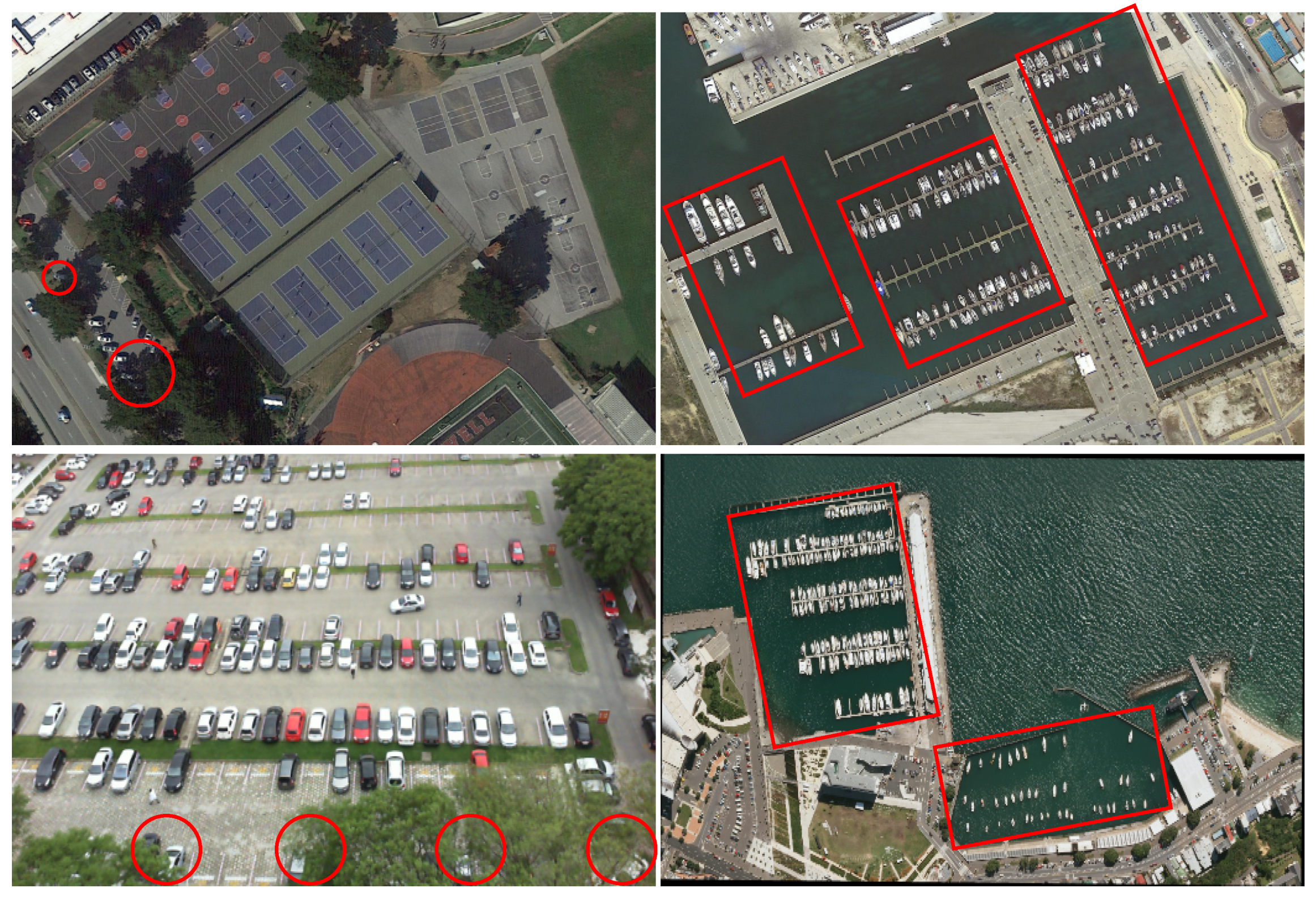
Some examples of objects with scale variation and background clutter in remote sensing images are depicted in Figure 1. The first column shows the challenges of background clutter. Remote sensing images are taken from the sky, and some vehicles may be sheltered under trees (enclosed by red circles), so it is necessary to accurately identify targets. The second column displays the problem of scale variation (the ships marked in red bounding boxes). One can see that the size varies obviously in the images due to the different types of ships. Thus, the counting model should possess the capacity of capturing large-range scale information.

To mitigate the background clutter, a simple yet effective tool is the visual attention mechanism, which can adjust the weights between the foreground and background. Gao et al. [17] introduced a dual attention module containing channel and spatial units to identify the foreground. Moreover, SwinCounter [13] was proposed to capture global context information based on the Swin Transformer. Specifically, the SwinCounter leverages several shifted windows to compute self-attention with others, which can highlight the tiny object region. Similarly, the PSGCNet [16] deployed a global context module to overcome the background noise by building dependencies between different channels.

To cope with the problem of scale variation, most solutions adopt multiple columns networks to capture multiscale information. For example, MCNN [15] is built to extract multiscale information with a three-branch architecture for crowd counting. Different filters are employed in each column to acquire various receptive fields. Furthermore, several different mechanisms, e.g., dilated convolution [12] and spatial pyramid pooling [18], are employed to boost the scale diversity. Chen et al. [19] leveraged four parallel dilated convolution layers to capture pyramid features to tackle the scale variation. Dai et al. [12] utilized some dense blocks with dense connections to obtain different features with multiple scales. Gao et al. [16] deployed a two-path module, where a local path with a pyramid architecture is built to capture multiscale information, and a global path is developed to capture the features of the large objects.

In this paper, a triple attention and scale-aware network (TASNet) is built to simultaneously address the problems of background clutter and scale variation in remote sensing images. First, a TVA module is proposed to address the problem of background clutter. It is built in a three-branch pattern, with each branch generating a refined feature by performing an attention operation across different dimensions. Then, the optimized features are averaged to generate the output tensor. In this way, the TVA module can boost the dependencies between the channel and spatial dimensions, which helps distinguish the foreground from the background. To relieve the adverse effect of scale variation, a PFA module is built with a four-branch structure. The four branches possess a similar configuration, which adopts dilated convolution to extract the multiscale information. Moreover, a scale transmit mechanism is introduced, which enables the upper branch to pass the scale cue to the lower branch to increase the scale diversity. Overall, the contributions are as follows:

• A triple attention scale-aware network (TASNet) is built in a divide-and-conquer manner to address the problem of background clutter and scale variation for object counting in remote sensing images.
• A TVA module, which executes attention operations on features in three views, is built to deal with the background clutter. A PFA module adopting a four-branch architecture is proposed to capture multiscale information.
• Extensive experiments are carried out to verify the performance of object counting in challenging remote sensing scenarios. Meanwhile, detailed ablation studies are conducted to prove the effectiveness of the different compound modes, backbone networks and the multiscale feature fusion mechanisms within the proposed model.

2. Related Literature

In this section, we present the related work in background clutter and scale variation, which are the two inevitable challenges in object counting in remote sensing.

2.1. Solutions for Background Clutter

Rich context information can guide the model to emphasize the foreground region and suppress background noise. The attention mechanism fits the bill and has been a powerful tool in object counting [20,21]. For example, Gao et al. [22] deployed two parallel attention modules (channel and spatial attention) to build a crowd counting network. Specifically, channel attention aims to alleviate the error estimation of complex backgrounds, while spatial attention can guide the model to perceive global information. Zhu et al. [23] built a dual path network consisting of a density map path for predicting a coarse map, and an attention map path to generate a head probability map. With the assistance of the probability map, the final density map can distinguish the head region from the background. Gao et al. [17] introduced a concatenated attention module to fuse multiscale features and restrain the background clutter. It first employs a channel unit to recognize the object area and then adopts a spatial unit to divide different density levels for encoding a wide range of dependencies. Jiang et al. [24] built an attention scaling network to recognize different density regions, which are generated by multiplying attention masks and scaling factors.

In addition to the assistance of the attention mechanism, many semantic segmentation methods are adopted to address the problem of background clutter. For example, Khan et al. [25] directly employed a scene segmentation framework for crowd counting. It is composed of three components, namely a classification module, semantic scene segmentation (SSS) module and density estimation module. Specifically, the SSS module can produce a segmentation map to highlight the head region. Meng et al. [26] proposed a regularized surrogate task based on binary segmentation. With the help of binary segmentation, the network can generate a hard uncertainty map and a soft uncertainty map to suppress the background noise. Gao et al. [27] designed a foreground and background segmentation (FBS) module to recognize the interest region. The FBS module is built with an encoder–decoder structure to produce a segmentation map, which is transmitted to the density head branch to emphasize the crowd region. Liu et al. [28] built several inter-related segmentation maps to assist predicting the high-quality density map. Specifically, for each segmentation map, the predicted values higher than the given threshold value are set to one; otherwise, they are set to zero.

However, the attention modules adopted in these networks still have weaknesses in transmitting information to each other, leading to weak dependencies between global and local perspectives. To this end, we build a TVA module into the network to enhance the dependencies among different dimensions.

2.2. Solutions for Scale Variation

Scale variation is another inevitable challenge limiting the improvement of counting performance. Many attempts have been devoted to addressing this problem. Zhang et al. [15] proposed the first multi-column network with diverse filter kernels to address this problem. Cao et al. [29] employed different filters to take scale features and then aggregate them as the input of the next layer. In addition to using a multi-column architecture, dilated convolution has been adopted to capture multiscale information. Li et al. [30] made full use of the dilated convolution and built a congested scene recognition (CSR) network to enlarge the receptive fields while saving the computation parameters. Liu et al. [31] introduced a structured feature representation learning mechanism to promote the complementarity between different scale feature maps. Meanwhile, a hierarchically structured loss function was proposed to boost the local correlation of different regions. Chen et al. [19] built a scale pyramid module (SPM) which contains four convolution layers with different dilated rates (2, 4, 8, 12) to extract multiscale features. Liu et al. [32] designed a contextual aware network (CAN) to enhance the counting performance. It encodes local scale feature maps and perceives different head sizes. Zhu et al. [33] proposed a multi-level features aggregation network. It consists of a key component termed scale and level aggregation module (SLAM). The SLAM first utilizes a four-branch scale aggregation (SA) to extract the multiscale information and then utilizes a channel attention (CA) to adjust the channel weights of each feature. Finally, the outputs of SA and CA are summed to generate multiscale features. Dai et al. [12] deployed three successive residual dense blocks to learn local and global context information. Duan et al. [34] embedded a context aggregation module (CAM) into the network to fuse multiscale context information. Moreover, the proposed module can retain tiny details by several pixel attention modules subsequently. Han et al. [35] designed a tree-like scale diversity module, which contains nine different sizes of receptive fields to extract scale features. In addition, a cross-scale communication is introduced to boost the complementary scale information fusion. Chen et al. [36] proposed a multiscale semantic refining module to solve the scale variation.

Unfortunately, the aforementioned methods have some limitations and weaknesses. For example, the dependencies of the global and local information should be built considering the independence of each column in a multi-column architecture. To this end, we introduce a modified multi-column module to enhance the dependencies of each column.

3. Methodology

3.1. Network Architecture

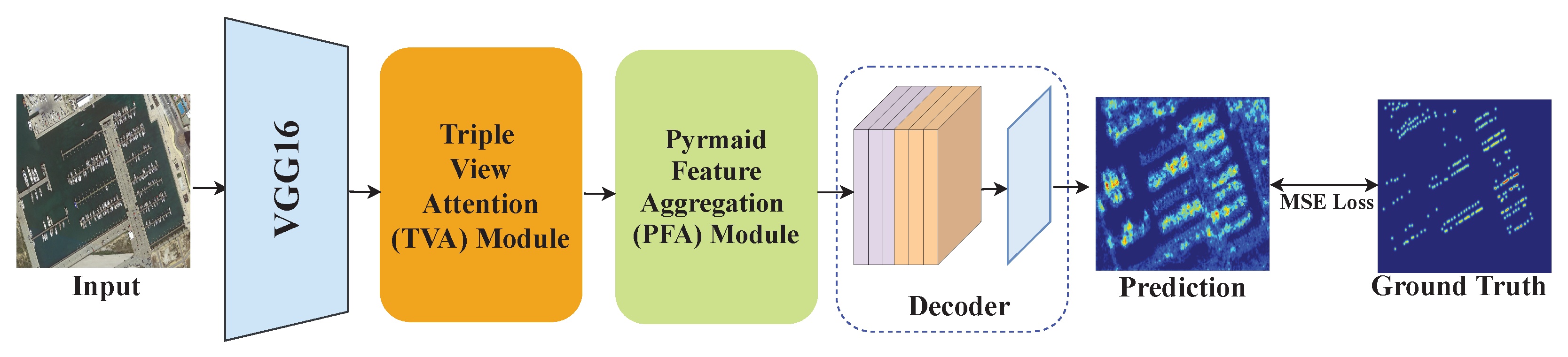
The architecture of the proposed TASNet is depicted in Figure 2. It comprises four parts, i.e., a backbone for basic feature extraction, a TVA module for identifying the object region, a PFA module for suppressing the scale variation, and a decoder for generating the final prediction.

Specifically, the tailored VGG16 [37] (with ten convolution layers and three max pooling layers) is selected as the backbone. This way, the output feature size is reduced to 1/4 of the input. Subsequently, the TVA module is built to mitigate the background clutter with a three-branch architecture. Afterward, the PFA module is utilized to extract the scale information through a multi-column structure. Lastly, a decoder including three successive convolution layers (3 × 3 kernel size with 512 channels), three deformable convolution layers (3 × 3 kernel sizes with 512, 256, and 128 channels), and a 1 × 1 convolution are equipped to generate the final density map. The prediction is supervised by the ground truth density map generated by the Gaussian kernel, and the MSE loss is applied to measure the $l_2$ distance between the two maps.

3.2. TVA Module

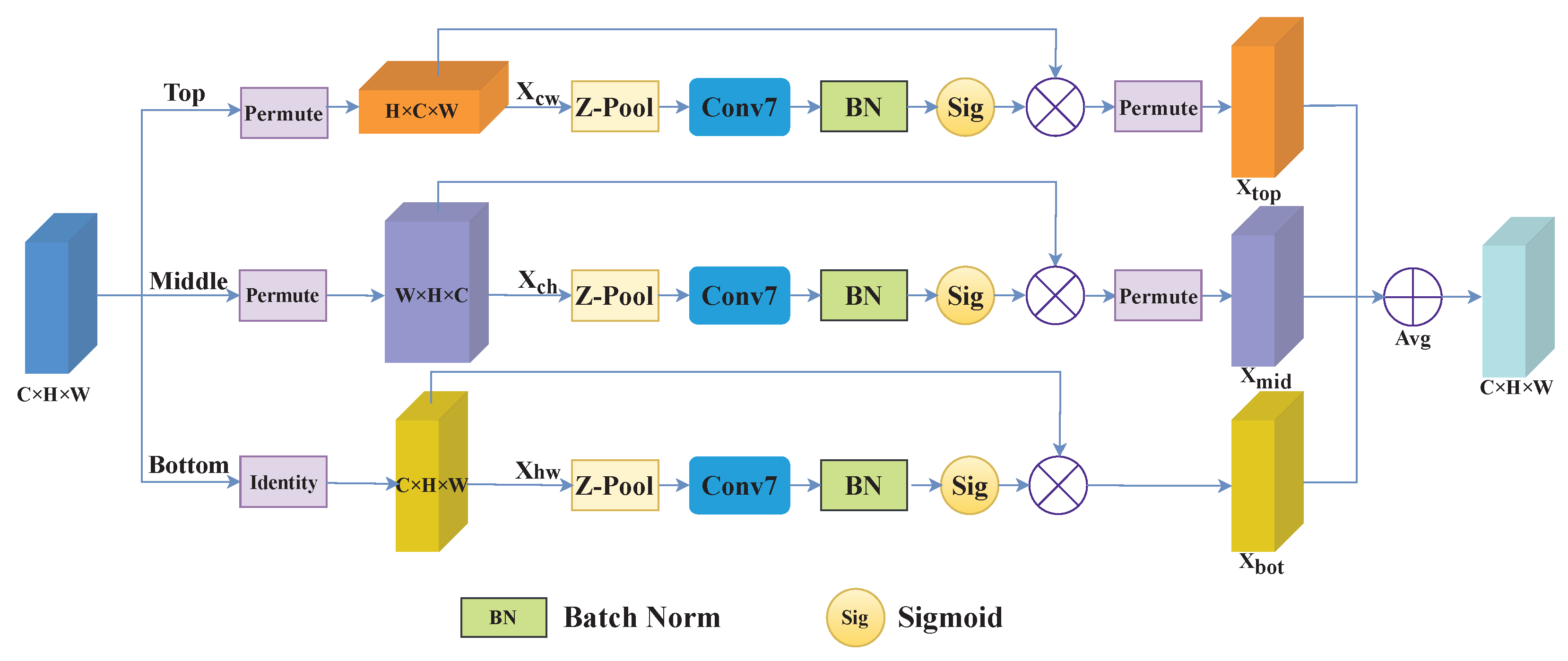
The complex background in remote sensing images may mislead the network to identify the object incorrectly, which weakens the counting performance. Therefore, we propose a triple view attention (TVA) module to deal with the challenge. Figure 3 exhibits the architecture of the TVA module.

For an input $\mathbf{X}\in {\mathbb{R}}^{C\times H\times W}$, three branches are established to perform attention operations on different dimensions and output three intermediate features. The three intermediate outputs are averaged to generate the final results.

Specifically, the goal of the top branch is to build the dependencies between the width dimension spatially and the channel dimension. First, the input is viewed as a new shape ${\mathbf{X}}_{\mathbf{cw}}\in {\mathbb{R}}^{H\times C\times W}$. Then, ${\mathbf{X}}_{\mathbf{cw}}$ is performed through a Z-pool operation [38], which aims to retain rich details and squeeze the depth of the height dimension spatially. The Z-pool is executed by combining the max pooled and average pooled features and reduces the zeroth dimension to 2. Mathematically, it is formulated as

$$Z\text{-}pool\left(\mathbf{X}\right)=\mathrm{Cat}\left(\mathrm{Maxpool}\right(\mathbf{X}),\mathrm{Avgpool}(\mathbf{X}\left)\right),$$

(1)

where Cat means the concatenate operation. Maxpool and Avgpool denote the operators of max pooling and average pooling, respectively. Afterward, the compressed tensor is fed into a standard convolution layer with a kernel size of k (set to 7 in this paper). Next, a batch normalization layer is added to compress the zeroth dimension to 1. The optimized weights can be obtained by a sigmoid function and are applied to ${\mathbf{X}}_{cw}$. Finally, the output ${\mathbf{X}}_{top}\in {\mathbb{R}}^{C\times H\times W}$ of the top branch is acquired and re-viewed as the shape of input $\mathbf{X}\in {\mathbb{R}}^{C\times H\times W}$. In sum, the top branch can be represented as,

$${\mathbf{X}}_{top}={\mathbf{X}}_{cw}\odot \mathrm{Sig}\left(\mathrm{BN}\left(\mathrm{Conv}\left(z_{pool}^{th}\left({\mathbf{X}}_{cw}\right)\right)\right)\right),$$

(2)

where BN and Sig are the batch normalization and sigmoid function, respectively. ⊙ is a dot product operation.

Like the top branch, the middle branch aims to build the dependencies between the spatial height dimension and channel dimension. It reshapes the input into ${\mathbf{X}}_{ch}\in {\mathbb{R}}^{W\times H\times C}$ and then performs the same operation as the top branch. Overall, it is formulated as,

$${\mathbf{X}}_{mid}={\mathbf{X}}_{ch}\odot \mathrm{Sig}\left(\mathrm{BN}\left(\mathrm{Conv}\left(z_{pool}^{th}\left({\mathbf{X}}_{ch}\right)\right)\right)\right),$$

(3)

The input of the bottom branch directly executes the attention operation compared with the upper branch. Following that, the same procedure is performed to obtain the attention result ${\mathbf{X}}_{hw}\in {\mathbb{R}}^{C\times H\times W}$. Then, the bottom branch can be formulated as,

$${\mathbf{X}}_{bot}={\mathbf{X}}_{hw}\odot \mathrm{Sig}\left(\mathrm{BN}\left(\mathrm{Conv}\left(z_{pool}^{th}\left({\mathbf{X}}_{hw}\right)\right)\right)\right),$$

(4)

The final feature ${\mathbf{X}}_{tva}\in {\mathbb{R}}^{C\times H\times W}$ is generated by averaging the outputs of three branches, which is formulated as,

$${\mathbf{X}}_{tva}=\frac{1}{3}({\mathbf{X}}_{top}+{\mathbf{X}}_{mid}+{\mathbf{X}}_{bot}).$$

(5)

3.3. PFA Module

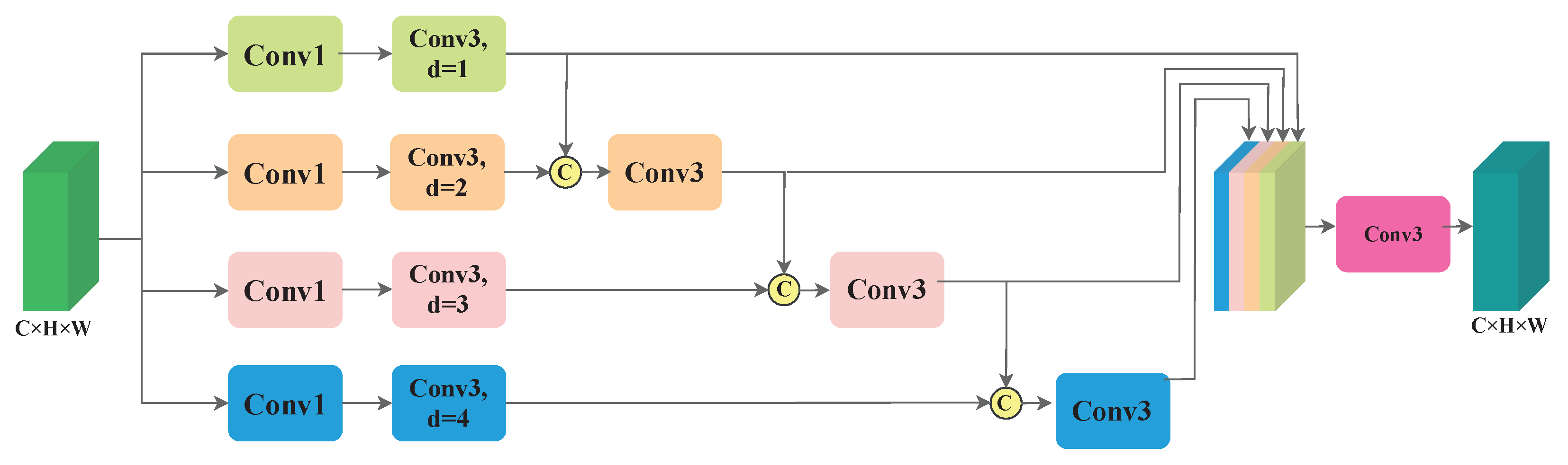
The scale variation in remote sensing images restrains the CNN from capturing large-range information of different sizes, which seriously degrades the estimated performance. To address this problem, a PFA module is built to extract wide-range scale features. The framework of the PFA module is depicted in Figure 4. It consists of a four-branch structure and a feature aggregation layer. The purpose of the four-branch structure is to capture multiscale information. Meanwhile, the feature aggregation layer aims to fuse the previously generated maps and compress the number of channels to be the same as the input.

Specifically, given an input ${\mathbb{R}}^{C\times H\times W}$, it is fed into the four-branch structure. In each branch, a 1 × 1 convolution layer is first utilized to compress the number of channels to 1/4 of the input feature. Afterwards, dilated convolution layers with dilated rates 1, 2, 3 and 4 are employed to enlarge the receptive field and form the pyramid features. Different from the previous multi-column networks [15,19], which extract information in each column separately, the proposed PFA module can transmit scale information from the upper branch to the lower branch. Particularly, the features of each branch are concatenated with the subsequent branch features. Then, a convolutional layer with a kernel size of 3 × 3 is subsequently deployed to fuse the features with diverse scales. Each branch is formulated as,

$$\left\{\begin{array}{cc}\hfill f_1& ={\mathrm{Conv}}_3^1\left(\mathrm{Compress}\left(\mathbf{X}\right)\right),\hfill \\ \hfill f_2& ={\mathrm{Conv}}_3^1\left(\mathrm{Cat}(f_1,{\mathrm{Conv}}_3^2\left(\mathrm{Compress}\left(\mathbf{X}\right)\right))\right),\hfill \\ \hfill f_3& ={\mathrm{Conv}}_3^1\left(\mathrm{Cat}(f_2,{\mathrm{Conv}}_3^3\left(\mathrm{Compress}\left(\mathbf{X}\right)\right))\right),\hfill \\ \hfill f_4& ={\mathrm{Conv}}_3^1\left(\mathrm{Cat}(f_3,{\mathrm{Conv}}_3^4\left(\mathrm{Compress}\left(\mathbf{X}\right)\right))\right),\hfill \end{array}\right.$$

(6)

where $f_1\sim f_4$ represents four intermediate features. $Con{v}_k^d$ denotes a convolution layer with filter size k and dilated rate d. Cat and Compress are the concatenate and compress operations, respectively.

The transition connection enables the lower branch to perceive multiscale information. Locally, the lower three branches can extract multiscale features. Globally, the PFA module enables the network to capture a wider scale range. Subsequently, a concatenate operation is executed on the generated feature map of each branch to aggregate them and generate a fused feature. Eventually, the output ${\widehat{\mathbb{R}}}^{C\times H\times W}$ is obtained by a 3 × 3 convolution layer. The PFA module is formulated as,

$${\mathbf{X}}_{pfa}={\mathrm{Conv}}_3\left(\mathrm{Cat}(f_1,f_2,f_3,f_4)\right),$$

(7)

3.4. Density Map Generation

To generate the ground truth density map, the dot map is filleted by a Gaussian function, which is the common criteria in the domain of object counting [15,39]. Supposing that the location of an object is at pixel $x_i$; then, it is defined by an impulse function $\delta (x-x_i)$. In this case, given a remote sensing image with N annotations, it can be defined as,

$$I\left(x\right)=\sum _{x=1}^N\delta (x-x_i),$$

(8)

Nevertheless, the density map generated is not continuous and cannot be employed to train the model. Therefore, the density map is converted into a continuous density function by convolving $I\left(x\right)$ with a Gaussian kernel $G_{{\sigma }_i}\left(x\right)$. The final density map can be formulated as,

$$D\left(x\right)=\sum _{i=1}^N\delta (x-x_i)\ast G_{{\sigma }_i}\left(x\right),$$

(9)

where ${\sigma }_i$ denotes the standard deviation of the Gaussian kernel. Following the previous work [17], we set $\sigma$ to 15.

3.5. Loss Function

The widely used “Mean Squared Error (MSE)” loss is adopted to train the model, which optimizes the model by minimizing the Euclidean distance between prediction and ground truth density maps. It is formulated as follows,

$$l\left(\theta \right)=\frac{1}{N}\sum _{i=1}^N{∥X_i^{Est}\left(\theta \right)-X_i^{GT}∥}_2^2,$$

(10)

where N represents the batch size, and $\theta$ denotes the parameters to be trained. $X_i^{GT}$ and $X_i^{Est}$ denote the ground truth map and estimated density map, respectively.

4. Experiments

4.1. Datasets

Remote Sensing Object Counting (RSOC) dataset: The RSOC dataset [17] is the largest remote sensing counting benchmark. Precisely, it consists of 3057 satellite images with a total of 286,539 annotations. It is further divided into four subdatasets based on the type of objects: buildings, small-vehicle, large-vehicle, and ship.

Car Parking Lot (CARPK) dataset: The CARPK dataset [40] includes 1448 drone-view images from four parking lots, of which 89,777 cars are labeled. The training and test sets contain 989 and 459 images, respectively.

Pontifical Catholic University of Paraná+ (PUCPR+) dataset: The PUCPR+ dataset [40] is a large-scale vehicle-counting dataset. The images are captured in parking lot scenes under different weather conditions, i.e., rainy, cloudy and sunny. In particular, it consists of 125 images with 16,456 annotations, among which 100 images are used for training and 25 images are used for testing, respectively. More details of the three datasets are listed in

Table 1. Detailed information of the RSOC, CARPK and PUCPR+ datasets.

Datasets	Platform	Images	Train/Test	Size (Avg.)	Annotation Format
RSOC_Building	Satellite	2468	1205/163	512 × 512	Center point
RSOC_Large-vehicle	Satellite	172	108/64	1552 × 1573	Bounding box
RSOC_Small-vehicle	Satellite	280	222/58	2473 × 2339	Bounding box
RSOC_Ship	Satellite	137	97/40	2558 × 2668	Bounding box
CARPK	Drone	1448	989/459	720 × 1280	Bounding box
PUCPR+	Camera	125	100/25	720 × 1280	Bounding box

.

4.2. Implementation Details

All experiments are implemented based on the PyTorch framework and executed on an NVIDIA 3090Ti GPU. During the training phase, the SGD optimizer with the initial learning rate of 1 × 10⁻⁷ and the decay rate of 5 × 10⁻⁴ is adopted to optimize the model. Furthermore, for high-resolution datasets, i.e., large-vehicle, small-vehicle, and ship, we resize them to 1024 × 768 in order to avoid out-of-memory.

For data augmentation, the crop size of the Building subdataset is set to 256 × 256, and the other three subdatasets in RSOC are set to 512 × 384. Then, we adopt mirror flipping to double them. Finally, the batch size is set to 32 for the Building dataset and 1 for the other datasets.

4.3. Evaluation Protocols

The widely used Mean Average Error (MAE) and Root Mean Squared Error (RMSE) are adopted [15,22] to evaluate the counting accuracy and robustness. They are formulated using,

$$MAE=\frac{1}{T}\sum _{i=1}^T\left|V_{est}^i-V_{gt}^i\right|,$$

(11)

$$RMSE=\sqrt{\frac{1}{T}\sum _{i=1}^T{\left|V_{est}^i-V_{gt}^i\right|}^2},$$

(12)

where T is the number of the test sample. $V_{est}^i$ and $V_{gt}^i$ denotes the estimated and ground truth value of the $i$-th image, respectively.

Meanwhile, we adopt the indicators of GFLOPs and runtime [27,41] to evaluate the efficiency of the models.

4.4. Experiments on the RSOC Dataset

The objective comparison results between the proposed method and SOTA methods on the RSOC dataset are presented in

Table 2. Comparative results on the RSOC dataset. The best and the second-best results are highlighted in red and blue, respectively.

Method	Building		Small-Vehicle		Large-Vehicle		Ship
	MAE	RMSE	MAE	RMSE	MAE	RMSE	MAE	RMSE
MCNN [15]	13.65	16.56	488.65	1317.44	36.56	55.55	263.91	412.30
CMTL [42]	12.78	15.99	490.53	1321.11	61.02	78.25	251.17	403.07
SANet [29]	29.01	32.96	497.22	1276.66	62.78	79.65	302.37	436.91
CSRNet [30]	8.00	11.78	443.72	1252.22	34.10	46.42	240.01	394.81
SCAR [22]	26.90	31.35	497.22	1276.65	62.78	79.64	302.37	436.92
SPN [19]	7.74	11.48	455.16	1252.92	36.21	50.65	241.43	392.88
CAN [32]	9.12	13.38	457.36	1260.39	34.56	49.63	282.69	423.44
SFCN [43]	8.94	12.87	440.70	1248.27	33.93	49.74	240.16	394.81
DSNet [12]	8.93	12.61	405.83	1254.16	27.44	42.38	206.25	346.96
SFANet [23]	8.18	11.75	435.29	1284.15	29.04	47.01	201.61	332.87
ASPDN [17]	7.54	10.52	433.23	1238.61	18.76	31.06	193.83	318.95
TASNet (Ours)	7.63	11.25	394.89	1196.83	22.75	37.13	191.82	278.17

.

One can see that the proposed TASNet achieves the best performance on the small-vehicle and ship datasets. Meanwhile, it achieves the second-best results on building and large-vehicle datasets. The possible reasons are that the building and large-vehicle datasets have more low-density scenarios than the small-vehicle and ship datasets. The proposed PFA module pays much more attention to the dense scenes, resulting in a suboptimal counting performance for sparse regions. Particularly, on the most challenging small-vehicle dataset, the TASNet improves the MAE by 20.5% and 9.3%, and RMSE by 6.3% and 4.1%, compared with SCAR [22] and SFANet [23], both of which adopt an attention mechanism to suppress the background clutter. On the ship dataset, the TASNet outperforms the ASPDN [17] in both MAE and RMSE. Although the results on building and large-vehicle datasets are the second best, the results are still competitive and convincing, especially compared with the multi-column networks, e.g., SANet [29] and SPN [19]. Notably, the small-vehicle and ship datasets are more challenging than the other two datasets in terms of background clutter and scale variation. Experimental results prove that the proposed method can well address these two problems and presents superior counting performance. Even so, there still exists a large improvement room on small-vehicle and ship datasets in accuracy and robustness.

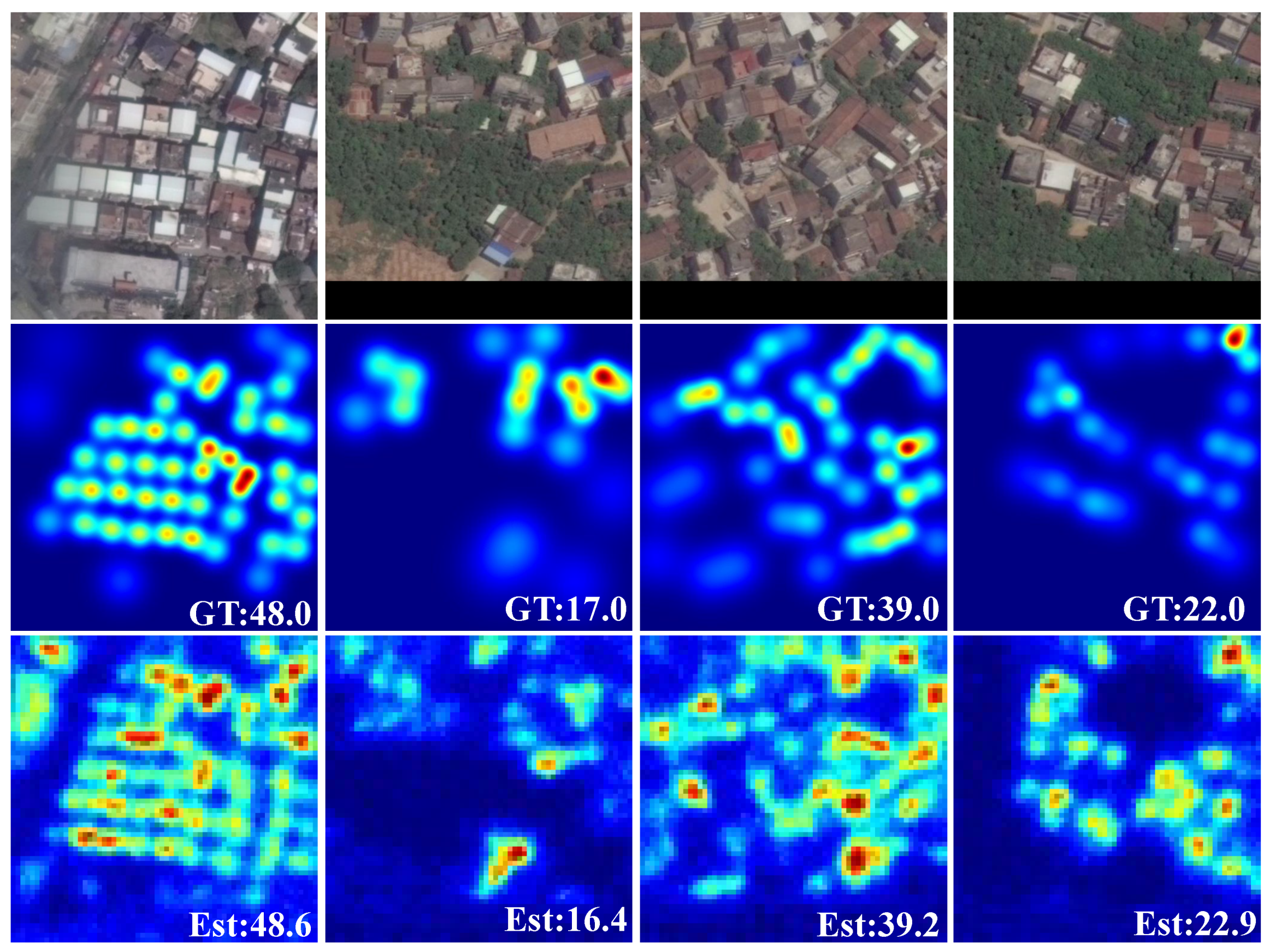
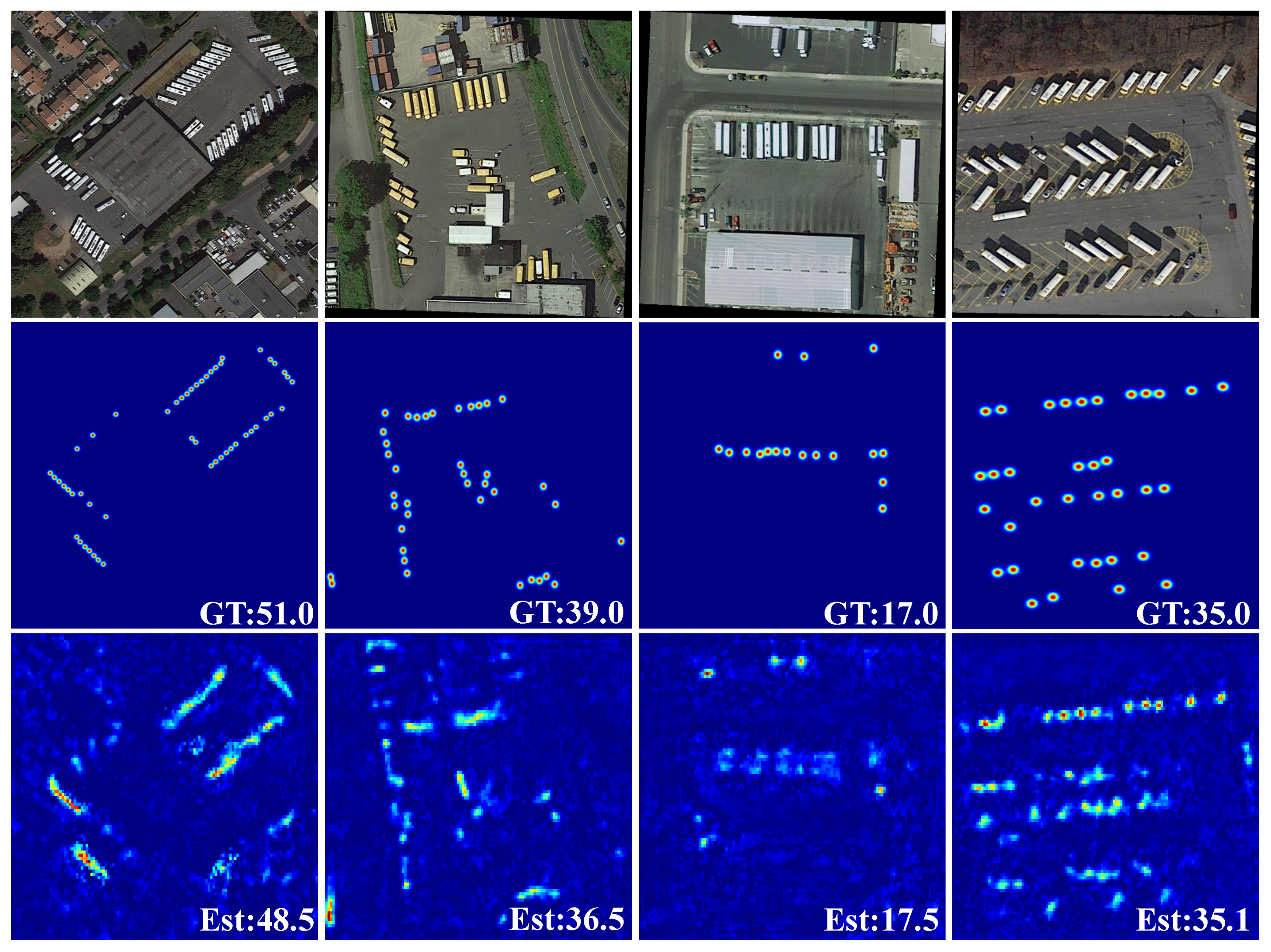
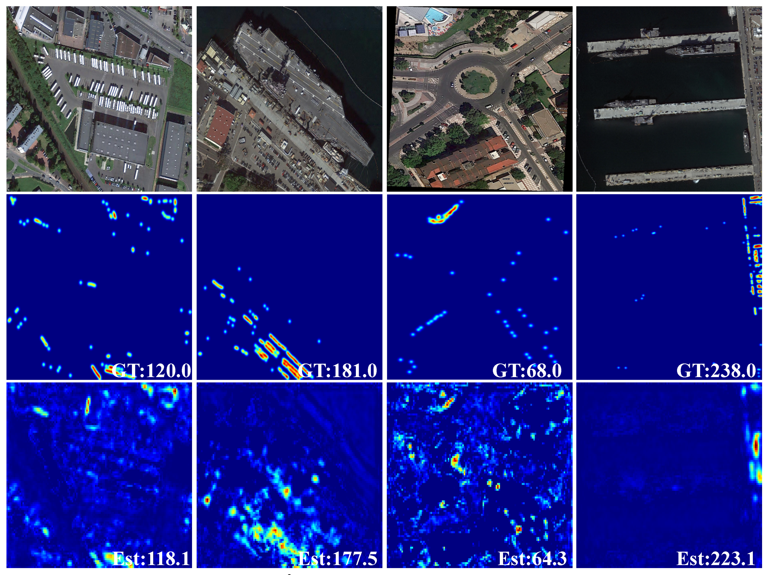
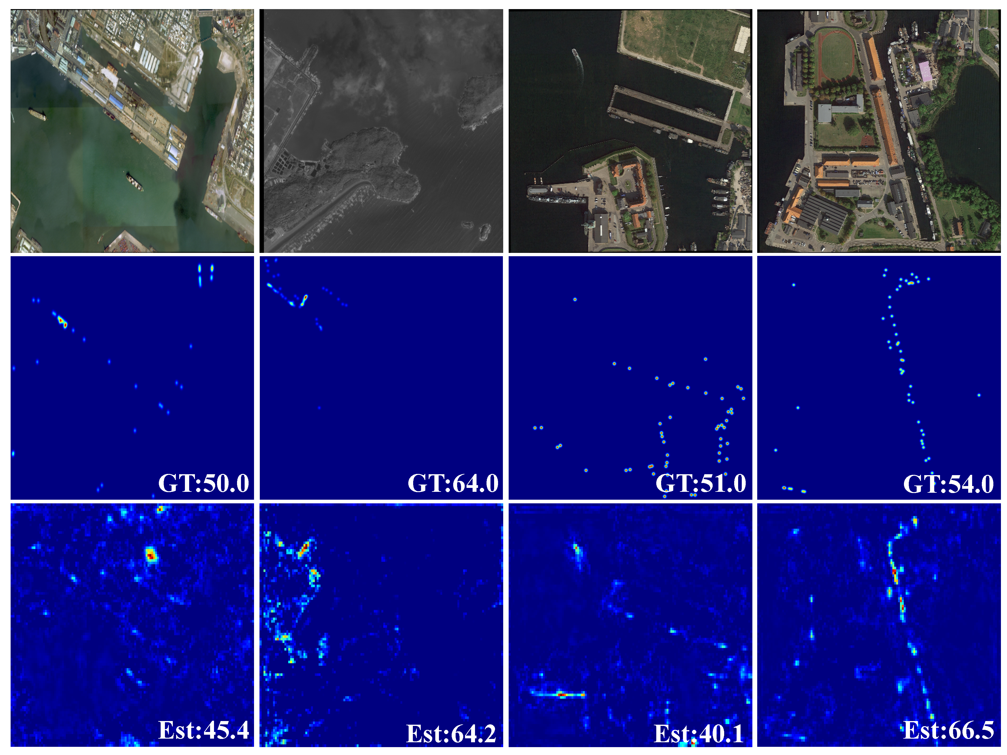
The visualization results on the four subdatasets of the RSOC dataset are presented in Figure 5, Figure 6, Figure 7 and Figure 8, respectively. Within these four figures, from top to bottom are the input remote sensing images, the corresponding ground truth density maps and the predicted density maps, where ‘GT’ and ‘Est’ denote the real value and estimated value, respectively. From the visualizations results, one can see that the estimated counting number and the density map are very close to ground truth.

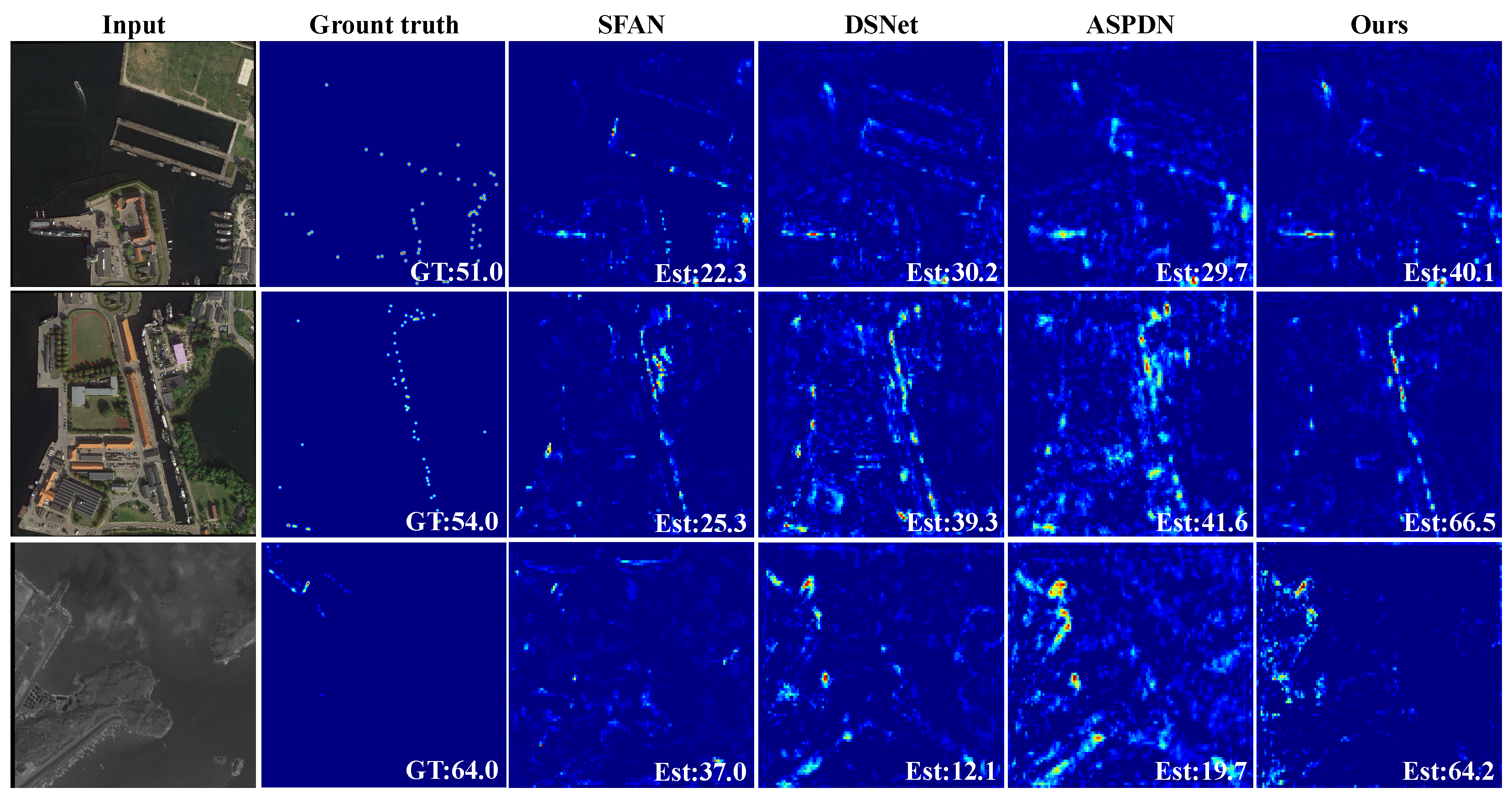
Some visual comparison of TASNet with other models (SFAN [23], DSNet [12] and ASPDN [17]) on the RSOC_ship dataset are illustrated in Figure 9. It proves that the TASNet can better handle the background clutter and scale variation than the other three methods. In addition, the estimated values are closer to ground truth compared with other methods.

4.5. Experiments on the CARPK Dataset

The objective comparison results on the CARPK dataset are shown in

Table 3. Experimental results on the CARPK and PUCPR+ datasets. The best and the second-best results are highlighted in red and blue, respectively.

Methods	CARPK		PUCPR+
	MAE	RMSE	MAE	RMSE
YOLO [9]	102.89	110.02	156.72	200.54
FRCN [44]	103.48	110.64	156.76	200.59
LEP [45]	51.83	-	15.17	-
LPN [40]	23.80	36.79	22.76	34.46
SSD [46]	37.33	42.32	119.24	132.22
RetinaNet [47]	16.62	22.30	24.58	33.12
One-Look Regression [48]	59.46	66.84	21.88	36.73
MCNN [15]	39.10	43.30	21.86	29.53
CSRNet [30]	11.48	13.32	8.65	10.24
BL [49]	9.58	11.38	6.54	8.13
PSGCNet [16]	8.15	10.46	5.24	7.36
TASNet (Ours)	7.16	10.23	5.16	6.76

.

The comparison methods fall into three categories, i.e., detection-based methods (from the first row to sixth row), regression-based methods (the seventh row) and deep learning-based methods (from the eighth row to eleventh row). Obviously, there is still a big margin between the first two methods and the deep learning-based methods. In addition, the counting performance of the regression-based method [48] is worse than that of most detection-based methods [40,45].

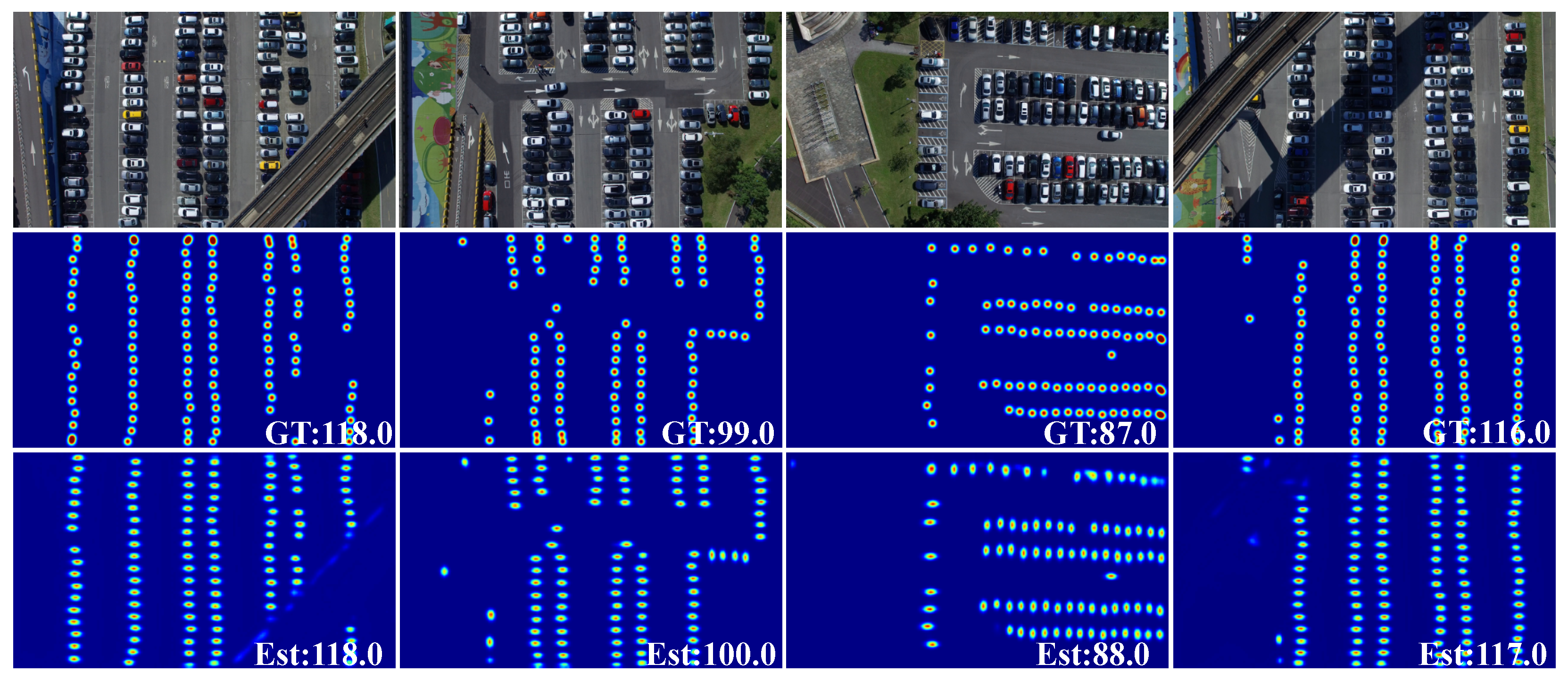
Compared with other deep learning methods, the proposed TASNet performs best in MAE and RMSE. Specifically, the TASNet achieved a score of 7.16 and 10.23 in MAE and RMSE, which are far ahead of the competitors. In particular, it improves the MAE by 12.1% compared with the PSGCNet [16], which is built specifically to cope with the problems of background clutter and scale variation. Figure 10 shows some visualized results on the CARPK dataset. One can see that the estimated maps are very close to the ground truth.

4.6. Experiments on the PUCPR+ Dataset

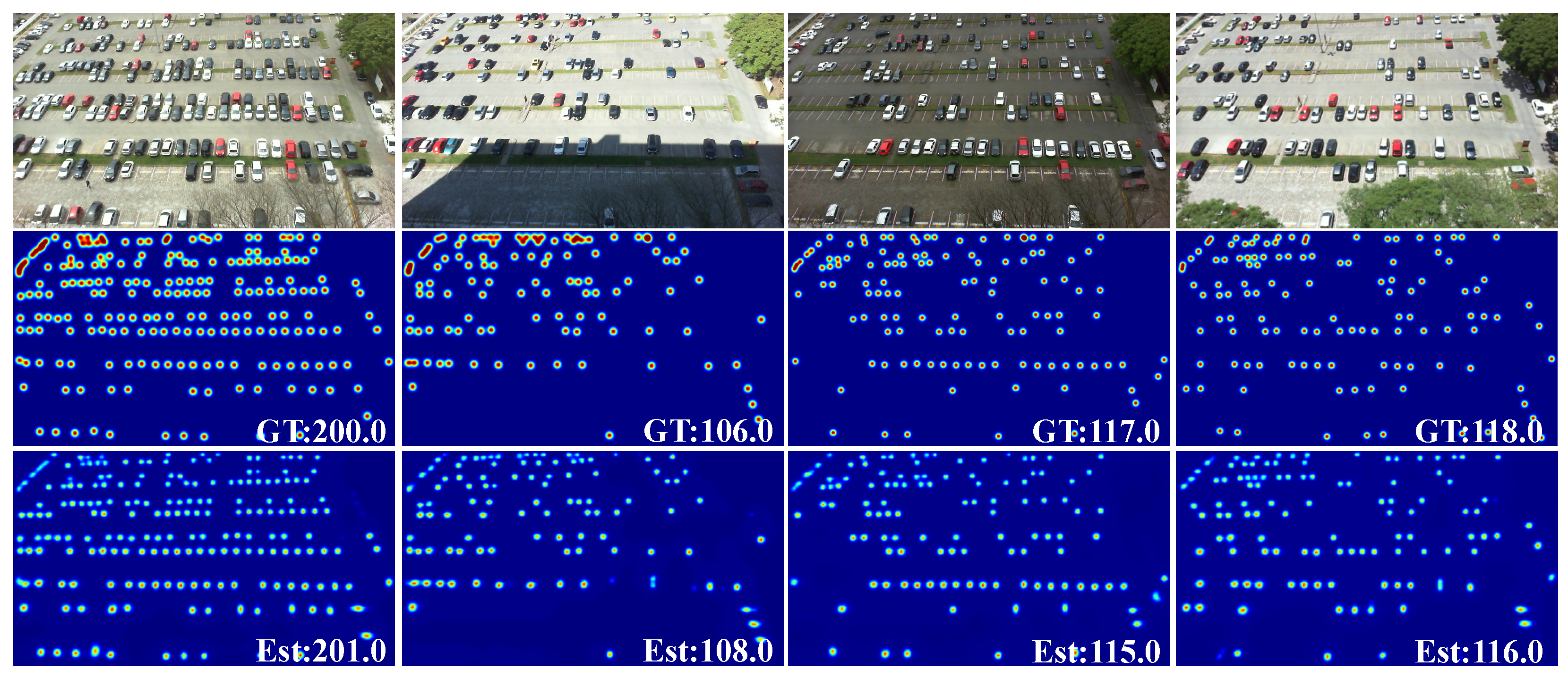
The objective comparison results on the PUCPR+ dataset are also shown in Table 3. Different from the CARPK dataset, the PUCPR+ dataset has a severe problem of weather variation, which is a big challenge for object counting. The experimental results show that the TASNet scores 5.16 in MAE and 6.76 in RMSE, which both outperform the competitors. Specifically, it reduces by 40.3% and 33.9% compared with CSRNet [30], which is proposed for addressing scale variation. Figure 11 shows some visualization results on the PUCPR+ datasets. It also verifies the effectiveness of the proposed TASNet in generating the density map and estimating the object counting.

4.7. Ablation Studies

In this section, we conduct a series of ablation studies to verify the different compound modes, the backbone networks, and the multiscale information fusion mechanisms.

4.7.1. Ablation Studies on the Modules

To trial the effectiveness of each module and the effect of different compound modes, we set up a series of ablation studies. The objective comparison results are listed in

Table 4. Comparative results of the baseline with different compound modes on the ship dataset. The best performances are highlighted in bold.

Methods	MAE	RMSE
Baseline	240.01	394.81
Baseline + TVA	237.88	373.97
Baseline + PFA	223.11	362.42
Baseline + PFA + TVA	214.22	312.35
Baseline+Parallel (TVA & PFA)	205.54	291.72
Baseline + TVA + PFA	191.82	278.17

. The configuration information and analysis are described below.

• Baseline: The baseline is considered as the pre-trained VGG16 with the decoder. It shows that the output results of the baseline are the worst.
• Baseline + TVA: The combination is to insert the TVA module between VGG16 and the decoder. One can see that the TVA module is beneficial in boosting the counting performance.
• Baseline + PFA: The group embeds the PFA module into the baseline. It proves that the PFA module is also conducive to the estimated performance.
• Baseline + PFA + TVA: Insert PFA and TVA modules successively in the baseline. It can be observed that the MAE and RMSE are improved by 10.7% and 20.9% compared with the baseline, respectively. It reveals that the combination of PFA and TVA modules is better than that of a single module.
• Baseline + Parallel (TVA and PFA): Connect the PFA and TVA modules in parallel and then add them to the baseline. Again, the results show that the performance improves more than the aforementioned compound modes.
• Baseline + TVA + PFA: Embed the TVA and PFA modules successively in the baseline. Intuitively, it exhibits the best performance in MAE and RMSE compared with all the configurations mentioned above.

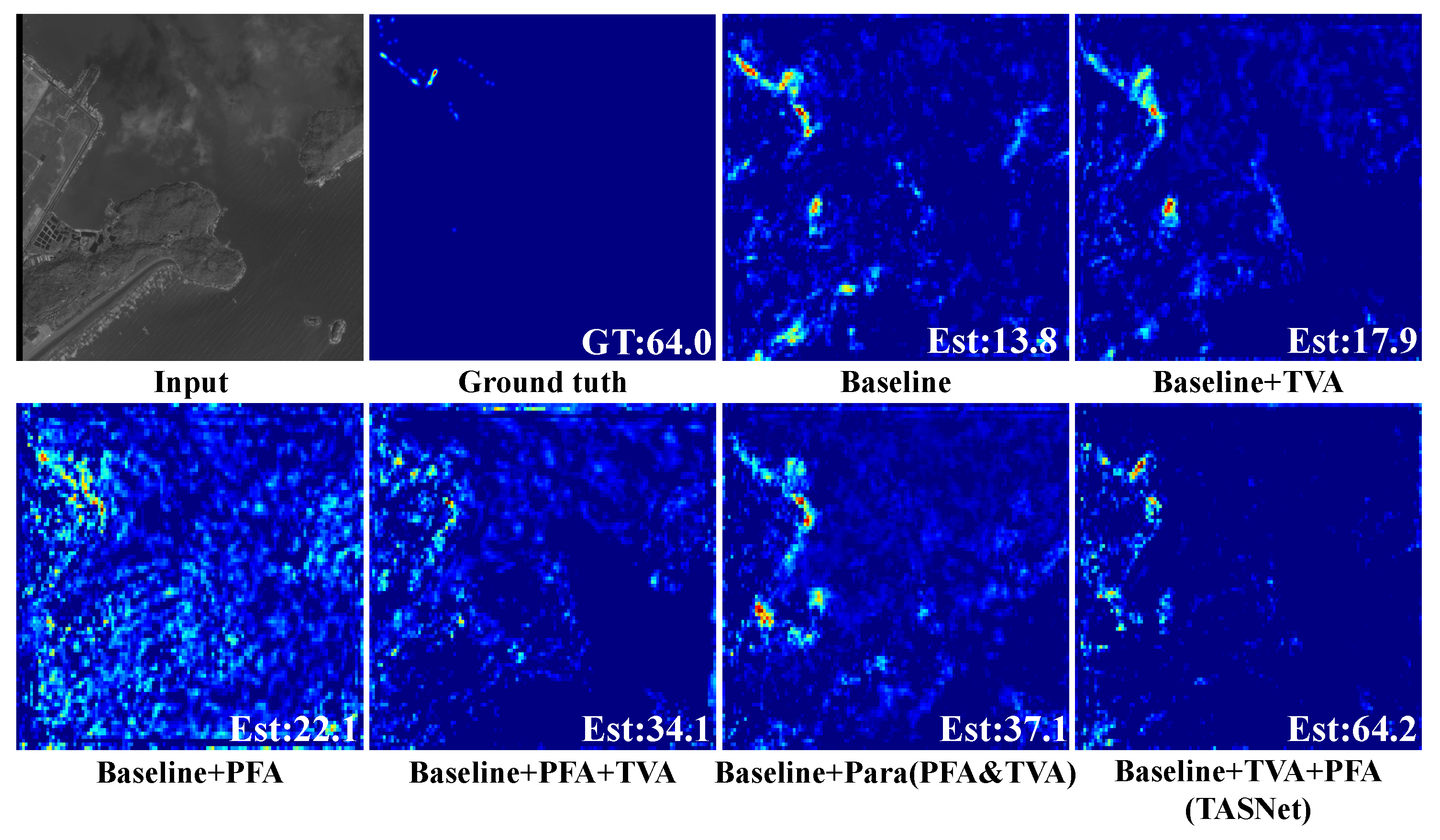
The visualization results of the baseline with different components are shown in Figure 12. It shows that both the TVA and PFA module are helpful to boost the counting performance. The proposed TVA module can effectively suppress the background noise. The PFA module can capture more large-scale information, but it incorrectly estimates other objects. Moreover, the problems of background clutter and scale variation are alleviated by adding the two modules to the baseline, but the compound mode of “Baseline + TVA + PFA” (TASNet) achieves the best results.

4.7.2. Ablation Studies on Backbone Networks

In addition to exploring the effectiveness of the proposed modules, ablation studies on backbone networks are also explored. Three networks, ResNet-50 [50], ResNeXt [51] and VGG-16, are adopted as backbone. The comparative results are shown in

Table 5. Comparative results of different backbones on the ship dataset. The best performances are highlighted in bold.

Methods	MAE	RMSE
TASNet (Resnet-50)	215.39	346.81
TASNet (ResneXt)	197.83	327.66
TASNet (VGG-16)	191.82	278.17

. It proves that adopting VGG-16 as the backbone network obtains the best performance. In fact, VGG is generally adopted as the backbone for feature extraction in most counting tasks [12,17,30] because of its strong generalization ability.

4.7.3. Ablation Studies on Multiscale Feature Fusion Mechanisms

In order to further prove the superiority of the proposed PFA module in multiscale feature fusion, three multiscale feature fusion mechanisms, namely scale pyramid module (SPM) [19], dense scale dilated convolution block (DDCB) [12] and pyramid scale module (PSM) [16], are compared. The comparative results are depicted in

Table 6. Comparative results of different multiscale feature fusion mechanisms on the ship dataset. The best performances are highlighted in bold.

Methods	MAE	RMSE
Baseline + TVA + SPM	192.69	329.45
Baseline + TVA + DDCB	194.48	294.46
Baseline + TVA + PSM	220.58	330.71
Baseline + TVA + PFA	191.82	278.17

. From the table, one can see that the PFA module is superior to the other three modules in multiscale information fusion. Specifically, compared with SPM and PSM which are built with pyramid structures, the proposed PFA module improves by 0.45% and 13.03% in MAE, and 15.51% and 15.89% in RMSE. Meanwhile, compared with DDCB, which is a single block with multiple dense connections, the PFA module reduces by 1.37% and 5.53% in MAE and RMSE. The advantage of the PFA module is that it introduces an information transmit mechanism in the pyramid structure which can capture more scale features.

4.8. Efficiency Comparison

To evaluate the efficiency of the proposed TASNet, we conduct comparative experiments to test the computational complexity and inferring time on an RTX 3090Ti GPU. The comparison results are reported in

Table 7. Comparison results of the TASNet and other models in parameters, GFLOPs and inferring time. The input size is set to $1024\times 768$.

Methods	Params (M)	GFLOPs	Inferring Time (ms)
SFANet [23]	17.0	312.83	34.1
DSNet [12]	20.7	379.15	34.5
ASPDN [17]	22.7	455.45	56.2
PSGCNet [16]	27.5	385.59	33.7
TASNet (Ours)	20.5	377.04	33.6

. One can see that the proposed TASNet scores 20.5 M and 377.04 in parameters and GFLOPs both achieving the second-best results among the competitors. Although the SFANet [23] ranks first in parameters and GFLOPs, it performs worse in counting accuracy and robustness than the TASNet (as shown in Table 2).

For the inferring time, the TASNet achieve 33.6, outperforming all competitors. Specifically, compared with the ASPDN [17], which performs best in the RSOC_building and RSOC_large-vehicle (as shown in Table 2), the TASNet improves by 40.2% in inferring time, which demonstrates that the TASNet is more efficient to ASPDN. In addition, the TASNet decreases by 1.4% compared with SFANet [23] with the least number of parameters, as it has a more bloated model.

4.9. Failure Cases

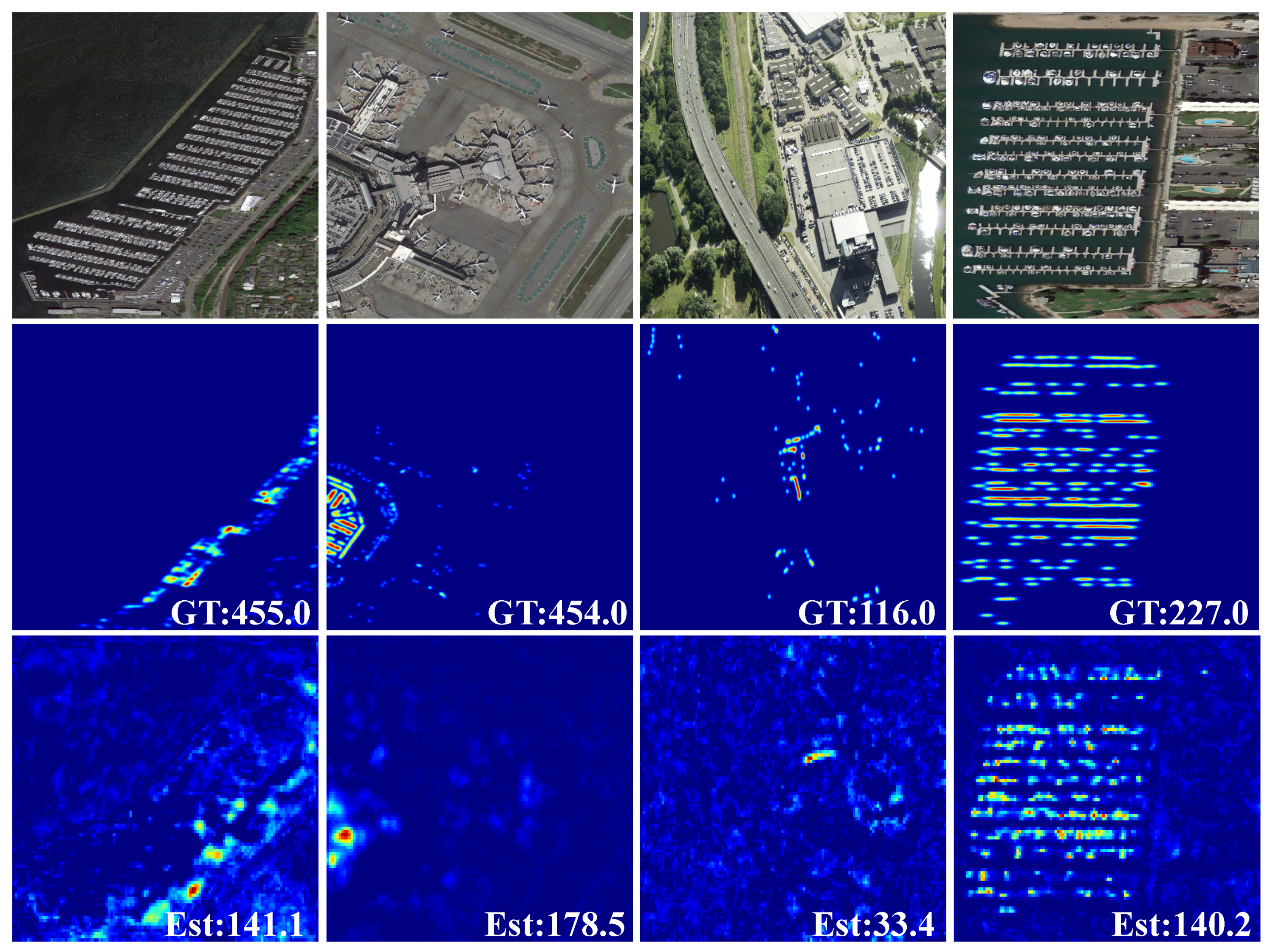
Although the proposed TASNet is capable of achieving the superior counting performance against other counting methods, it still has some failure cases, especially on the RSOC dataset. Some failure cases are visualized in Figure 13. One can see that there is a large gap between the estimated value and the ground truth, especially for tiny object counting in dense scenarios.

Tiny object counting is very valuable for real-world vision application and differs from general counting tasks. For instance, since the objects are tiny while the whole input image has a relatively large field-of-view, there is much less information from the targeting objects and much more from background distractions. The distinctions make tiny object counting a uniquely challenging task [52]. It indicates that there is still a large amount of room for tiny object counting.

5. Conclusions and Future Work

In this paper, we present the TASNet to address the problems of background clutter and scale variation for object counting in remote sensing. The proposed TASNet is characterized by two key components, i.e., a TVA module and a PFA module. Specifically, the TVA module is built to capture the dependencies of features across the spatial and channel dimensions. It can emphasize the object region and suppress the background noise. Meanwhile, the PFA module is introduced to solve the scale variation by extracting multiscale information with a four-branch architecture. Experimental results on extensive remote sensing datasets verified the effectiveness and superiority of the proposed TASNet. In the future, more efforts are expected to tiny object counting in dense scenarios, as the tiny objects have fewer detailed information and are highly susceptible to background interference.

References

- Zhang, Q.; Cong, R.; Li, C.; Cheng, M.M.; Fang, Y.; Cao, X.; Zhao, Y.; Kwong, S.T.W. Dense Attention Fluid Network for Salient Object Detection in Optical Remote Sensing Images. IEEE Trans. Image Process. 2021, 30, 1305–1317. [Google Scholar] [CrossRef]
- Gadamsetty, S.; Ch, R.; Ch, A.; Iwendi, C.; Gadekallu, T.R. Hash-Based Deep Learning Approach for Remote Sensing Satellite Imagery Detection. Water 2022, 14, 707. [Google Scholar] [CrossRef]
- Bazi, Y.; Bashmal, L.; Rahhal, M.M.A.; Dayil, R.A.; Ajlan, N.A. Vision Transformers for Remote Sensing Image Classification. Remote. Sens. 2021, 13, 516. [Google Scholar] [CrossRef]
- Zhang, S.; Yuan, Q.; Li, J.; Sun, J.; Zhang, X. Scene-Adaptive Remote Sensing Image Super-Resolution Using a Multiscale Attention Network. IEEE Trans. Geosci. Remote. Sens. 2020, 58, 4764–4779. [Google Scholar] [CrossRef]
- Rathore, M.M.; Ahmad, A.; Paul, A.; Rho, S. Urban planning and building smart cities based on the Internet of Things using Big Data analytics. Comput. Netw. 2016, 101, 63–80. [Google Scholar] [CrossRef]
- Grinias, I.; Panagiotakis, C.; Tziritas, G. MRF-based segmentation and unsupervised classification for building and road detection in peri-urban areas of high-resolution satellite images. Isprs J. Photogramm. Remote. Sens. 2016, 122, 145–166. [Google Scholar] [CrossRef]
- Benedek, C.; Descombes, X.; Zerubia, J. Building Development Monitoring in Multitemporal Remotely Sensed Image Pairs with Stochastic Birth-Death Dynamics. IEEE Trans. Pattern Anal. Mach. Intell. 2012, 34, 33–50. [Google Scholar] [CrossRef] [Green Version]
- Fan, Y.; Wen, Q.; Wang, W.; Wang, P.; Li, L.; Zhang, P. Quantifying Disaster Physical Damage Using Remote Sensing Data—A Technical Work Flow and Case Study of the 2014 Ludian Earthquake in China. Int. J. Disaster Risk Sci. 2017, 8, 471–488. [Google Scholar] [CrossRef]
- Redmon, J.; Divvala, S.K.; Girshick, R.B.; Farhadi, A. You Only Look Once: Unified, Real-Time Object Detection. In Proceedings of the 2016 IEEE Conference on Computer Vision and Pattern Recognition (CVPR), Las Vegas, NV, USA, 27–30 June 2016; pp. 779–788. [Google Scholar] [CrossRef] [Green Version]
- Girshick, R.B. Fast R-CNN. In Proceedings of the 2015 IEEE International Conference on Computer Vision (ICCV), Santiago, Chile, 7–13 December 2015; pp. 1440–1448. [Google Scholar] [CrossRef]
- Pham, V.Q.; Kozakaya, T.; Yamaguchi, O.; Okada, R. COUNT Forest: CO-Voting Uncertain Number of Targets Using Random Forest for Crowd Density Estimation. In Proceedings of the 2015 IEEE International Conference on Computer Vision (ICCV), Santiago, Chile, 7–13 December 2015; pp. 3253–3261. [Google Scholar] [CrossRef]
- Dai, F.; Liu, H.; Ma, Y.; Cao, J.; Zhao, Q.; Zhang, Y. Dense Scale Network for Crowd Counting. In Proceedings of the 2021 International Conference on Multimedia Retrieval, Tokyo, Japan, 22–24 March 2021. [Google Scholar] [CrossRef]
- Gao, J.; Gong, M.; Li, X. Global Multi-Scale Information Fusion for Multi-Class Object Counting in Remote Sensing Images. Remote. Sens. 2022, 14, 4026. [Google Scholar] [CrossRef]
- Gao, G.; Gao, J.; Liu, Q.; Wang, Q.; Wang, Y. CNN-based Density Estimation and Crowd Counting: A Survey. arXiv 2020, arXiv:2003.12783. [Google Scholar]
- Zhang, Y.; Zhou, D.; Chen, S.; Gao, S.; Ma, Y. Single-Image Crowd Counting via Multi-Column Convolutional Neural Network. In Proceedings of the IEEE Conference on Computer Vision and Pattern Recognition (CVPR), Las Vegas, NV, USA, 27–30 June 2016; pp. 589–597. [Google Scholar] [CrossRef]
- Gao, G.; Liu, Q.; Hu, Z.; Li, L.; Wen, Q.; Wang, Y. PSGCNet: A Pyramidal Scale and Global Context Guided Network for Dense Object Counting in Remote-Sensing Images. IEEE Trans. Geosci. Remote. Sens. 2022, 60, 1–12. [Google Scholar] [CrossRef]
- Gao, G.; Liu, Q.; Wang, Y. Counting From Sky: A Large-Scale Data Set for Remote Sensing Object Counting and a Benchmark Method. IEEE Trans. Geosci. Remote. Sens. 2021, 59, 3642–3655. [Google Scholar] [CrossRef]
- Lan, M.; Zhang, Y.; Zhang, L.; Du, B. Global context based automatic road segmentation via dilated convolutional neural network. Inf. Sci. 2020, 535, 156–171. [Google Scholar] [CrossRef]
- Chen, X.; Bin, Y.; Sang, N.; Gao, C. Scale Pyramid Network for Crowd Counting. In Proceedings of the 2019 IEEE Winter Conference on Applications of Computer Vision (WACV), Waikoloa, HI, USA, 7–11 January 2019; pp. 1941–1950. [Google Scholar] [CrossRef]
- Guo, X.; Gao, M.; Zhai, W.; Shang, J.; Li, Q. Spatial-Frequency Attention Network for Crowd Counting. Big Data 2022, 10, 453–465. [Google Scholar] [CrossRef] [PubMed]
- Zhai, W.; Gao, M.; Anisetti, M.; Li, Q.; Jeon, S.; Pan, J. Group-split attention network for crowd counting. J. Electron. Imaging 2022, 31, 41214. [Google Scholar] [CrossRef]
- Gao, J.; Wang, Q.; Yuan, Y. SCAR: Spatial-/channel-wise attention regression networks for crowd counting. Neurocomputing 2019, 363, 1–8. [Google Scholar] [CrossRef] [Green Version]
- Zhu, L.; Zhao, Z.; Lu, C.; Lin, Y.; Peng, Y.; Yao, T. Dual Path Multi-Scale Fusion Networks with Attention for Crowd Counting. arXiv 2019, arXiv:1902.01115. [Google Scholar]
- Jiang, X.; Zhang, L.; Xu, M.; Zhang, T.; Lv, P.; Zhou, B.; Yang, X.; Pang, Y. Attention Scaling for Crowd Counting. In Proceedings of the IEEE Conference on Computer Vision and Pattern Recognition (CVPR), Seattle, WA, USA, 13–19 June 2020; pp. 4705–4714. [Google Scholar] [CrossRef]
- Khan, K.; Khan, R.; Albattah, W.; Nayab, D.; Qamar, A.M.; Habib, S.; Islam, M. Crowd Counting Using End-to-End Semantic Image Segmentation. Electronics 2021, 10, 1293. [Google Scholar] [CrossRef]
- Meng, Y.; Zhang, H.; Zhao, Y.; Yang, X.; Qian, X.; Huang, X.; Zheng, Y. Spatial Uncertainty-Aware Semi-Supervised Crowd Counting. In Proceedings of the 2021 IEEE/CVF International Conference on Computer Vision (ICCV), Montreal, QC, Canada, 10–17 October 2021; pp. 15529–15539. [Google Scholar] [CrossRef]
- Gao, J.; Wang, Q.; Li, X. PCC Net: Perspective Crowd Counting via Spatial Convolutional Network. IEEE Trans. Circuits Syst. Video Technol. 2020, 30, 3486–3498. [Google Scholar] [CrossRef] [Green Version]
- Liu, Y.; Liu, L.; Wang, P.; Zhang, P.; Lei, Y. Semi-Supervised Crowd Counting via Self-Training on Surrogate Tasks. arXiv 2020, arXiv:2007.03207. [Google Scholar] [CrossRef]
- Cao, X.; Wang, Z.; Zhao, Y.; Su, F. Scale Aggregation Network for Accurate and Efficient Crowd Counting. In Proceedings of the European Conference on Computer Vision (ECCV), Munich, Germany, 8–14 September 2018. [Google Scholar] [CrossRef]
- Li, Y.; Zhang, X.; Chen, D. CSRNet: Dilated Convolutional Neural Networks for Understanding the Highly Congested Scenes. In Proceedings of the IEEE Conference on Computer Vision and Pattern Recognition (CVPR), Salt Lake City, UT, USA, 18–23 June 2018; pp. 1091–1100. [Google Scholar] [CrossRef] [Green Version]
- Liu, L.; Qiu, Z.; Li, G.; Liu, S.; Ouyang, W.; Lin, L. Crowd Counting With Deep Structured Scale Integration Network. In Proceedings of the 2019 IEEE/CVF International Conference on Computer Vision (ICCV), Seoul, Republic of Korea, 27 October–2 November 2019; pp. 1774–1783. [Google Scholar] [CrossRef] [Green Version]
- Liu, W.; Salzmann, M.; Fua, P. Context-Aware Crowd Counting. In Proceedings of the IEEE Conference on Computer Vision and Pattern Recognition (CVPR), Long Beach, CA, USA, 15–20 June 2019; pp. 5094–5103. [Google Scholar] [CrossRef]
- Zhu, F.; Yan, H.; Chen, X.; Li, T.; Zhang, Z. A multi-scale and multi-level feature aggregation network for crowd counting. Neurocomputing 2021, 423, 46–56. [Google Scholar] [CrossRef]
- Duan, Z.; Wang, S.; Di, H.; Deng, J. Distillation Remote Sensing Object Counting via Multi-Scale Context Feature Aggregation. IEEE Trans. Geosci. Remote. Sens. 2022, 60, 1–12. [Google Scholar] [CrossRef]
- Han, K.; Wang, Y.; Tian, Q.; Guo, J.; Xu, C.; Xu, C. GhostNet: More Features From Cheap Operations. In Proceedings of the 2020 IEEE/CVF Conference on Computer Vision and Pattern Recognition (CVPR), Seattle, WA, USA, 13–19 June 2020; pp. 1577–1586. [Google Scholar] [CrossRef]
- Chen, J.; Wang, K.; Su, W.; Wang, Z. SSR-HEF: Crowd Counting With Multiscale Semantic Refining and Hard Example Focusing. IEEE Trans. Ind. Inform. 2022, 18, 6547–6557. [Google Scholar] [CrossRef]
- Simonyan, K.; Zisserman, A. Very Deep Convolutional Networks for Large-Scale Image Recognition. arXiv 2015, arXiv:1409.1556. [Google Scholar]
- Misra, D.; Nalamada, T.; Arasanipalai, A.U.; Hou, Q. Rotate to Attend: Convolutional Triplet Attention Module. In Proceedings of the 2021 IEEE Winter Conference on Applications of Computer Vision (WACV), Waikoloa, HI, USA, 3–8 January 2021; pp. 3138–3147. [Google Scholar] [CrossRef]
- Zhai, W.; Gao, M.; Souri, A.; Li, Q.; Guo, X.; Shang, J.; Zou, G. An attentive hierarchy ConvNet for crowd counting in smart city. Clust. Comput. 2022. [Google Scholar] [CrossRef]
- Hsieh, M.R.; Lin, Y.L.; Hsu, W.H. Drone-Based Object Counting by Spatially Regularized Regional Proposal Network. In Proceedings of the International Conference on Computer Vision (ICCV), Venice, Italy, 22–29 October 2017; pp. 4165–4173. [Google Scholar] [CrossRef] [Green Version]
- Wang, P.; Gao, C.; Wang, Y.; Li, H.; Gao, Y. MobileCount: An efficient encoder-decoder framework for real-time crowd counting. Neurocomputing 2020, 407, 292–299. [Google Scholar] [CrossRef]
- Sindagi, V.; Patel, V. CNN-Based cascaded multi-task learning of high-level prior and density estimation for crowd counting. In Proceedings of the IEEE International Conference on Advanced Video and Signal Based Surveillance (AVSS), Lecce, Italy, 29 August–1 September 2017; pp. 1–6. [Google Scholar] [CrossRef] [Green Version]
- Wang, Q.; Gao, J.; Lin, W.; Yuan, Y. Learning From Synthetic Data for Crowd Counting in the Wild. In Proceedings of the IEEE Conference on Computer Vision and Pattern Recognition (CVPR), Long Beach, CA, USA, 15–20 June 2019; pp. 8190–8199. [Google Scholar] [CrossRef]
- Ren, S.; He, K.; Girshick, R.B.; Sun, J. Faster R-CNN: Towards Real-Time Object Detection with Region Proposal Networks. TPAMI 2015, 39, 1137–1149. [Google Scholar] [CrossRef] [PubMed] [Green Version]
- Stahl, T.; Pintea, S.L.; Gemert, J.C.V. Divide and Count: Generic Object Counting by Image Divisions. IEEE Trans. Image Process. 2019, 28, 1035–1044. [Google Scholar] [CrossRef]
- Liu, W.; Anguelov, D.; Erhan, D.; Szegedy, C.; Reed, S.E.; Fu, C.Y.; Berg, A.C. SSD: Single Shot MultiBox Detector. In Proceedings of the European Conference on Computer Vision (ECCV), Amsterdam, The Netherlands, 11–14 October 2016; pp. 21–37. [Google Scholar] [CrossRef] [Green Version]
- Lin, T.Y.; Goyal, P.; Girshick, R.B.; He, K.; Dollár, P. Focal Loss for Dense Object Detection. IEEE Trans. Pattern Anal. Mach. Intell. 2020, 42, 318–327. [Google Scholar] [CrossRef] [Green Version]
- Mundhenk, T.N.; Konjevod, G.; Sakla, W.A.; Boakye, K. A Large Contextual Dataset for Classification, Detection and Counting of Cars with Deep Learning. In Proceedings of the European Conference on Computer Vision (ECCV), Amsterdam, The Netherlands, 11–14 October 2016. [Google Scholar] [CrossRef] [Green Version]
- Ma, Z.; Wei, X.; Hong, X.; Gong, Y. Bayesian Loss for Crowd Count Estimation With Point Supervision. In Proceedings of the 2019 IEEE/CVF International Conference on Computer Vision (ICCV), Seoul, Republic of Korea, 27 October–2 November 2019; pp. 6141–6150. [Google Scholar] [CrossRef] [Green Version]
- He, K.; Zhang, X.; Ren, S.; Sun, J. Deep Residual Learning for Image Recognition. In Proceedings of the 2016 IEEE Conference on Computer Vision and Pattern Recognition (CVPR), Las Vegas, NV, USA, 27–30 June 2016; pp. 770–778. [Google Scholar] [CrossRef] [Green Version]
- Xie, S.; Girshick, R.B.; Dollár, P.; Tu, Z.; He, K. Aggregated Residual Transformations for Deep Neural Networks. In Proceedings of the 2017 IEEE Conference on Computer Vision and Pattern Recognition (CVPR), Honolulu, HI, USA, 21–26 July 2017; pp. 5987–5995. [Google Scholar] [CrossRef] [Green Version]
- Yu, X.; Han, Z.; Gong, Y.; Jan, N.; Zhao, J. The 1st Tiny Object Detection Challenge: Methods and Results. In Proceedings of the 2020 ECCV Workshops, Glasgow, UK, 23–28 August 2020. [Google Scholar] [CrossRef]
Figure 1.
Examples of objects with scale variation and background clutter in remote sensing.
Figure 2.
Architecture of the TASNet for object counting in remote sensing.
Figure 3.
Architecture of the TVA module.
Figure 4.
Architecture of the PFA module.
Figure 5.
Subjective results on the RSOC_building dataset.
Figure 6.
Subjective results on the RSOC_large-vehicle subdataset.
Figure 7.
Subjective results on the RSOC_small-vehicle subdataset.
Figure 8.
Subjective results on the RSOC_ship subdataset.
Figure 9.
Subjective comparisons of different models on the RSOC_ship subdataset.
Figure 10.
Subjective results on the CARPK dataset.
Figure 11.
Subjective results on the PUCPR+ dataset.
Figure 12.
The qualitative comparison of the baseline with different components.
Figure 13.
Failure cases on the RSOC dataset.