
Assessment of Spatio-Temporal Empirical Forecasting Performance of Future Shoreline Positions

Department of Geography, Virginia Polytechnic Institute and State University, Blacksburg, VA 24061, USA
*
Author to whom correspondence should be addressed.
Remote Sens. 2022, 14(24), 6364; https://0-doi-org.brum.beds.ac.uk/10.3390/rs14246364
Submission received: 14 October 2022
/
Revised: 8 December 2022
/
Accepted: 14 December 2022
/
Published: 16 December 2022
(This article belongs to the Special Issue Remote Sensing of the Aquatic Environments-Part II)
Abstract
:Coasts and coastlines in many parts of the world are highly dynamic in nature, where large changes in the shoreline position can occur due to natural and anthropogenic influences. The prediction of future shoreline positions is of great importance in the better planning and management of coastal areas. With an aim to assess the different methods of prediction, this study investigates the performance of future shoreline position predictions by quantifying how prediction performance varies depending on the time depths of input historical shoreline data and the time horizons of predicted shorelines. Multi-temporal Landsat imagery, from 1988 to 2021, was used to quantify the rates of shoreline movement for different time period. Predictions using the simple extrapolation of the end point rate (EPR), linear regression rate (LRR), weighted linear regression rate (WLR), and the Kalman filter method were used to predict future shoreline positions. Root mean square error (RMSE) was used to assess prediction accuracies. For time depth, our results revealed that the higher the number of shorelines used in calculating and predicting shoreline change rates the better predictive performance was yielded. For the time horizon, prediction accuracies were substantially higher for the immediate future years (138 m/year) compared to the more distant future (152 m/year). Our results also demonstrated that the forecast performance varied temporally and spatially by time period and region. Though the study area is located in coastal Bangladesh, this study has the potential for forecasting applications to other deltas and vulnerable shorelines globally.
1. Introduction
Globally, coastal areas are vulnerable to different natural hazards, including floods, erosion, hurricanes, cyclones, tsunami, and saltwater intrusion, because of their proximity to the sea. These hazards are responsible for extensive economic, social, ecological, and human losses [1]. According to the United Nations [2], approximately 40% of the world’s population lives within 60 miles of the coast, which is expected to grow significantly in the future. Continued climate change and sea-level rise is expected to substantially impact the people living in coastal areas [3,4]. Sea level rise poses serious threats for the people living in the coastal zone, which leads to coastal erosion, inundations in the low-lying areas, tidal water encroachment and subsequent salt-water intrusion, as well as the displacement of the people living along the coast.
Coastal erosion is one of the biggest problems in the coastal areas globally, and the world’s mega deltas are heavily affected [5]. During the twentieth century, the mean sea level rose by 11–16 cm [6,7], possibly exacerbating coastal erosion globally. Due to rising seas, the resulting inundation will heavily impact low-lying areas; impacting at least 100 million persons globally who live within one meter of the mean sea level [8]. Coastal Bangladesh is highly vulnerable to coastal erosion, where land accretion and erosion are among the highest in the world [9,10,11,12]. It is a recurring problem, causing thousands of people to become homeless every year [13]. Economically challenged populations living in coastal areas are among the most severely impacted victims of such changes. Additionally, the magnitudes and severities of the affected people and their associated livelihoods may affect the total economic growth of the country [14]. Due to coastal erosion, people living on the coast not only lose their agricultural land but also their infrastructure, communication systems, and most importantly their livelihoods. For a lower middle-class country, such as Bangladesh, with limited internal resources, it is hard to cope with catastrophic natural hazards, such as coastal erosion and its related consequences [15].
The detection of shoreline movement and prediction of future shoreline position is important for the informed management of the coastal zone and to limit the structural and financial losses in the coast [16]. Due to the dynamic nature of physical coastal processes, the prediction of future shorelines can be particularly challenging. Shoreline retreat (erosion) and advance (accretion) can depend on many factors and processes, including fluvial discharge, bathymetry, land cover along the littoral, wind and wave energy, rainfall, sea level rise, human alterations (e.g., protective structures), and acute disturbance events such as cyclones [17,18]. There are two general approaches to shoreline prediction. First, researchers have used physically based process models that involve various geophysical input parameters (e.g., discharge, wave energy) [19,20]. Coastal geoscientists and engineers often apply this approach. A second approach employs empirically based, data-driven statistical methods that do not involve process models or simulations. This type of prediction uses the historical observations of erosion/accretion rates to predict future scenarios [21,22]. Geospatial scientists commonly use this approach.
Remote sensing and GIS-based techniques are useful and widely used by coastal researchers in detecting and predicting coastal erosion and accretion [10,23,24]. The Digital Shoreline Analysis System (DSAS) is one of the most used toolkits in detecting shoreline movement. The DSAS toolkit is an ArcGIS plugin developed by the United States Geological Survey [25]. In this research, we adopted an empirically based, data-driven approach of shoreline prediction using DSAS to derive rates of shoreline positional change. Historical change rates have been often been used to predict future shorelines by employing statistical extrapolation [26,27]. In this approach, the key inputs are historical change rates derived from satellite imagery.
Among the methods used, the end point rate (EPR) is one of the most widely used method due to its relative ease to use employing two mapped shorelines for two dates and no requirement of additional data or use of a physically-based model [28]. The linear regression rate (LRR) and weight linear regression rate (WLR) described below employ multiple shoreline dates with the associated regression techniques. To obtain the predicted future shorelines, simple extrapolation extends a terminal date shoreline to some date in the future via the simple extrapolation of the observed historical rates of shoreline positional change. The Kalman filter method is an alternative approach for future shoreline prediction. The main difference between the Kalman filter method and simple extrapolation is that the Kalman filter method is a recursive algorithm that employs multiple steps applied to estimates of the current state variable (e.g., EPR) at each successive time step, along with its uncertainty [29]. The outcome of successive estimates of future shoreline movement, which includes spatial uncertainty and random noise, is updated using a weighted average with more weight being given to estimates with a higher certainty. A recent study by Ciritci and Turk [21] used the Kalman filter method to compare the prediction accuracy alternatively using the end point rate (EPR), linear regression rate (LRR), and weighted linear regression (WLR) as inputs using a future prediction time horizon of 10 and 20 years. Results suggested that using the WLR shoreline change rate as input to the Kalman filter prediction method provided more accurate results than with the use of the other rates (e.g., EPR, LRR).
The main goal of this research is to assess the variability of future shoreline prediction performance depending on the time depth of input predictor data (e.g., number of annual historical shoreline observations) and the forecast horizon of predicted future shorelines (e.g., the number of years into the future that are predicted). Compared to much of the coastal erosion literature, this work uses a richer time series dataset derived from a 34-year time series of satellite-derived shorelines at annual temporal resolution. This time depth enables us to employ a temporal strategy to yield a robust characterization of the space-time patterns of shoreline change and future shoreline prediction. It enables us to empirically assess the performance of the future shoreline position predictions by quantifying how the prediction performance varies depending on the time depths of the input historical shoreline data and the time horizons of predicted shorelines. This is a methodological innovation with the potential for forecasting applications to other deltas and vulnerable shorelines globally. While empirical results are specific to the project’s study area, results can inform the region’s shoreline forecasting ability and associated mitigation and adaptation strategies.
The specific objectives of this study are to (1) assess how coastal erosion/accretion varies spatially and temporally, (2) measure how predictive performance varies over space and time, (3) examine how successful the empirical forecasting of future shoreline positions is, (4) evaluate how well alternative extrapolation methods of shoreline prediction perform, and (5) identify what time depths of historical predictor shorelines and what time horizons of future predicted shorelines yield the best predictive performance.
2. Materials and Methods
2.1. Study Area
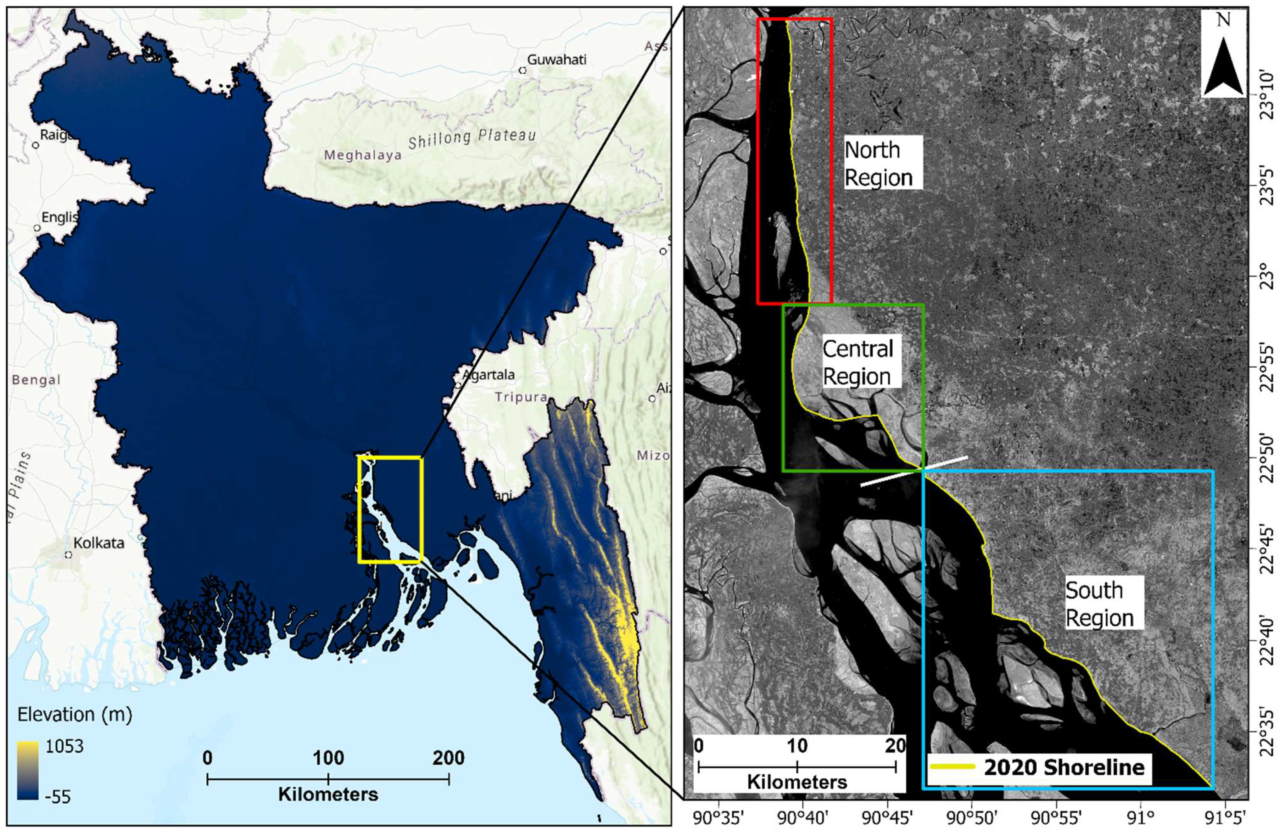
The study area is located along the eastern bank of the lower Meghna River, near the Bay of Bengal (Figure 1). This part of the delta is morphologically very dynamic in nature. The Meghna River is an alluvial meandering river which confluences with the Padma River at the upstream of our study area. Its shoreline spans the coastal upazilas (local administrative regions equivalent to US counties) of Chandpur and Lakshmipur, districts of Bangladesh. The upazilas are the second lowest tier of administrative unit. According to the population census of 2011, more than two million people live in the study area’s six upazilas. Most households depend on agriculture or fishing for their livelihoods [30,31]. This study covers more than 85 km of shoreline along the eastern bank of the lower Meghna Estuary. According to previous studies [11,12], this part of the estuary is highly vulnerable to coastal erosion due to the heavy discharge of sediment flow from the upstream of one of the largest deltas in the world, named the Ganges–Brahmaputra–Meghna (GBM) delta. People living in this low-lying coast are very close to the sea level with an average elevation of 5 m.
2.2. Data
This study analyzed satellite data for a period of 34 years from 1988 to 2021. Multi-temporal Landsat satellite data was obtained from the USGS Earth Explorer website (https://earthexplorer.usgs.gov/, accessed on 2 May 2021). Landsat imagery is widely used for quantification of coastal erosion [10,11,32,33]. In order to obtain cloud-free imagery, satellite images were selected and downloaded for the dry season winter months (December to February) every year. A detailed description of the imagery used can be found in Table A1 of Appendix A.
2.3. Methods
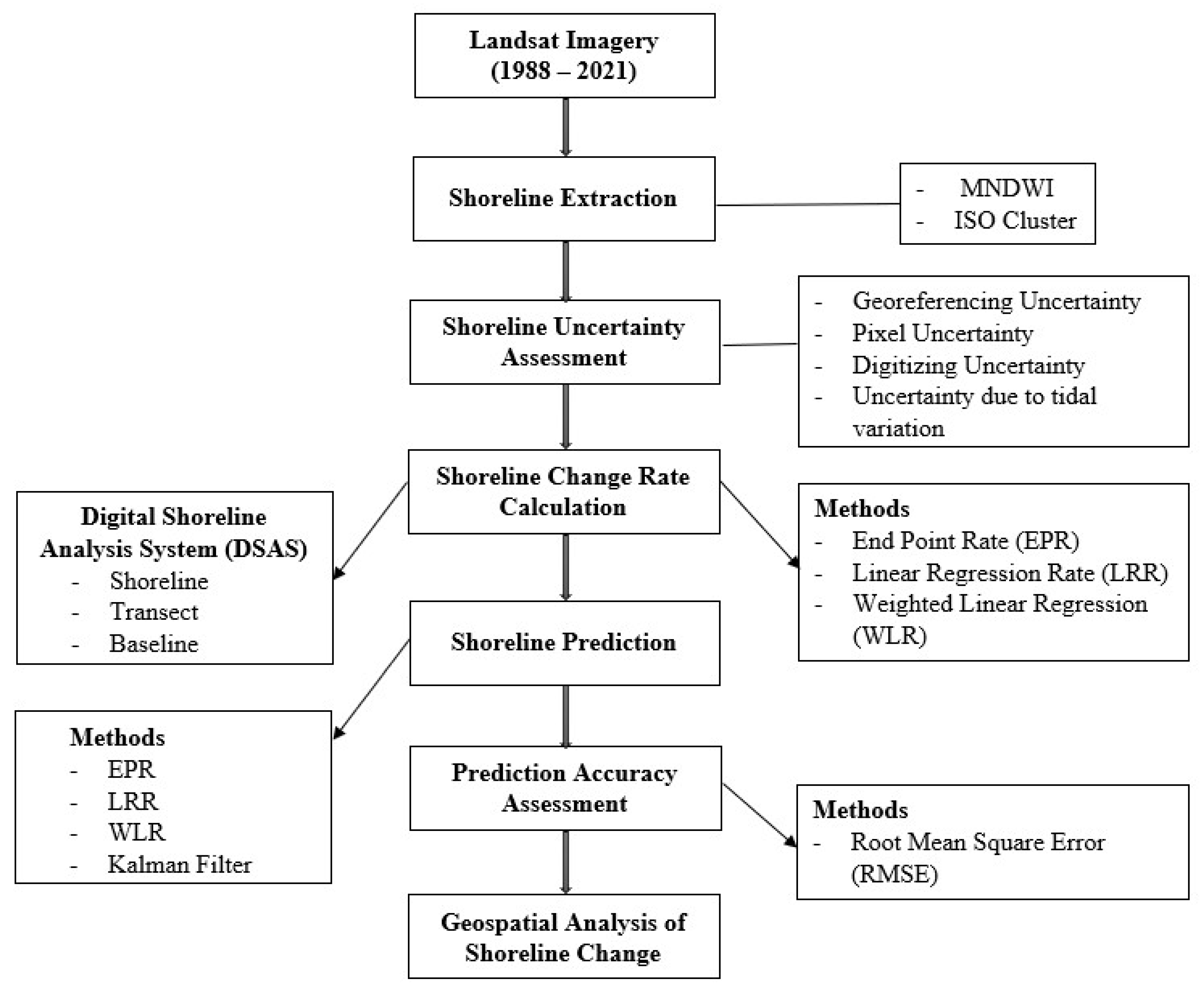
In this study, shoreline prediction performance was analyzed using the aforementioned Landsat time-series data of 1988–2021. Satellite images were processed using ArcGIS Pro software. The Digital Shoreline Analysis System (DSAS) was used to calculate shoreline change rates, and simple extrapolation and the Kalman filter method were used to predict future shoreline positions. First, images were preprocessed using ArcGIS Pro. Second, annual shoreline positions were extracted (e.g., vector shorelines) and shoreline uncertainties were assessed. Third, using DSAS, shoreline change rates were calculated. Finally, shoreline change rates were used to predict future shoreline positions and prediction accuracy was assessed. A detailed diagram of the work flow used in this study can be found in Figure 2.
2.3.1. Shoreline Extraction
To extract annual shorelines, the Modified Normalized Difference Water Index (MNDWI) were used as an input with other Landsat bands. The middle infrared (MIR) and green bands are used to create this index which enhances the ability to distinguish between open water features while suppressing/removing other noises, such as built-up land, vegetation, and soil noise [34]. MNDWI is defined as:
The MNDWI value ranges from −1 to 1, where water pixels approach to 1, and are easily distinguishable from other pixels. It is a widely used method to separate water and non-water pixels. After getting the index, the ISO cluster unsupervised classification was used to classify the images into 10 classes. In this process, we used red, green, blue, and MIR bands, along with MNDWI as an input. After obtaining the initial ISO cluster classification output layer, the output layers were reclassified into two classes, water and non-water via visual interpretation. The land–water interface defining shoreline was then converted to a vector digital shoreline employing a smoothing algorithm. Results yielded annual dry season shorelines for every year from 1988 to 2021.
2.3.2. Shoreline Uncertainty
The accurate estimation of shoreline errors and uncertainties is necessary. The accuracy of the shoreline movement estimation is affected by several factors. This study assessed and accounted for four uncertainty terms provided by Hapke et al. [35].
Shoreline uncertainty was assessed using the following equation:
where, Utotal = total uncertainty, Ug = georeferencing uncertainty, Up = pixel uncertainty, Ud = digitizing uncertainty, and Ut = uncertainty associated with tide.
Georeferencing uncertainty (Ug) of the Landsat imagery used varied from 3.5 m to 7.3 m. This information was obtained from the metadata provided with the imagery. Pixel uncertainty (Up) is related to the pixel resolution of the imagery. All imagery we used had a 30 m resolution. That said, the pixel uncertainty (Up) was 30 m for all the images used in this study. The uncertainty related to the manual digitizing of shorelines from visual inspection is typically defined as digitizing uncertainty (Ud). Since we used the automated shoreline digitization method, our digitizing uncertainty (Ud) value is 0. To assess uncertainty due to tidal variation (Ut), we adopted the same approach used in our previous research [12]. Six different shorelines were derived for the dry season of 2000 using Landsat imagery. We found that the tidal levels ranged from 0.8 m to 2.8 m for the dates/times of the analyzed images. To measure the shoreline position difference, depending on the tide level, fifteen different combinations of shorelines for each transect were quantified. Our calculation suggested that the mean tidal difference was 0.97 m. We used regression analysis to reveal the shoreline uncertainty. Our analysis of shoreline uncertainty exhibits 1 m tidal difference, resulting in a 7 m shoreline shift. As a result, we applied a tidal uncertainty of 7 m. A detailed summary of the shoreline uncertainty assessment can be found in Table 1.
2.3.3. Shoreline Change Rates Calculation
Shoreline change rates were calculated using the DSAS (Digital Shoreline Analysis System), a software package for the quantification of shoreline movement developed by United States Geological Survey [25]. The EPR, LRR, and WLR were used to calculate the shoreline change rates at a 95% confidence interval. The EPR rate is calculated by dividing the distance of shoreline movement by the time period between the oldest and the most recent shoreline [29], yielding a change rate in units of meters per year. EPR is one of the most widely used methods for shoreline change rate calculation [23,36]. The LRR rate is calculated by fitting a least-squares regression line to all shoreline points for digital transects that are cast orthogonal from an offshore or onshore baseline to the mapped shorelines. With the x-axis being time (e.g., year), and the y-axis being the distance from the baseline to the observed shorelines, the regression coefficient and its uncertainty is an estimate of the true shoreline change rate and its associated uncertainty. This method is applied to the set of transects such that each transect obtains a transect-specific shoreline change rate and uncertainty value. In practice, it is common to use a transect spacing of 50 m; the spacing adopted here resulted in 1551 transects spanning the ~85 km shoreline of the study areas. Similarly, the WLR rate is calculated by fitting a least-squares regression line to all shoreline points for each transect by taking into consideration the uncertainty values associated with measurement [29]. In a weighted linear regression, the more reliable data are given greater emphasis or weight towards determining a best-fit line. The weight (w) is defined as a function of the variance in the uncertainty of the measurement (e).
where, e is shoreline uncertainty value.
2.3.4. Shoreline Prediction and Temporal Strategy
For the shoreline prediction, we have used both simple extrapolation and Kalman filter methods, which take shoreline change rates as input, such as the EPR, LRR, and WLR. Prediction involves a general two-step process. For the simple extrapolation of historical rates, ArcGIS, via relevant geoprocessing tools, was used. We also calculated the advanced form of extrapolation using the Kalman filter method using the DSAS software. In short, for each of the 1551 digital transects, a “terminal shoreline position”, which is the x, y location of the intersection of the transect with an empirically mapped digital shoreline (e.g., shoreline derived from Landsat) for the year from which a future shoreline position prediction is made, is shifted either onshore or offshore depending on the empirically derived shoreline change rate which may be either positive or negative indicating shoreline accretion or erosion. In this way, a predicted future shoreline position along each transect for a defined time horizon into the future is produced.
Important to this research is the establishment of a temporal strategy to predict future shorelines. This is important to satisfy our goal and the innovation of evaluating how prediction performance varies over time and space. Our strategy required consideration of both the time depth of historical shorelines (e.g., how many years of annual input shorelines) used to quantify historically observed shoreline change rates and the time horizon for future prediction shorelines (e.g., how far out in the future to predict). We used time depths of 5, 10, and 15 years in the past and time horizons of 1, 5, 10, and 20 years into the future.
As described below, we used the LRR rates for all shoreline predictions using both the simple extrapolation and Kalman filter methods. In the case of Kalman filter prediction, we could not predict future shoreline positions using 5-year time depth data due to technical issues with the DSAS, though we were able to do so for 10 year and 15-year time depth data. A large dataset was generated in combination of four different methods of prediction, three different time depths and four different time horizons. Approximately 300k observations were produced at the transect level through the above combinations where digital transects at 50 m spacing were cast orthogonal from a digital baseline such that transects intersected the shorelines at approximately 90 degrees. Through our previous research [11] and personal observation, we found that the central zone of our study produced some noise in generating data due to the nature of the complexity of erosion and accretion in this region. As a result, we state that some transects at the central region will result in large rates of shoreline positional change that are statistical outliers. We, therefore, trimmed to remove these outliers from the data. Based on empirical data inspection, we excluded transects with change rates exceeding 500 m/year. Through this process, we removed approximately 2.4% of the observations from the final data analysis.
2.3.5. Prediction Performance Metric
Empirical prediction of future shorelines requires metrics to evaluate prediction accuracy. Prior research [21,26,27] has used the root mean square error metric (RMSE) to measure prediction accuracy, a common measure of accuracy assessment across science domains. The RMSE is the standard deviation of the residuals (prediction error). To assess the prediction accuracy, this study used RMSE as a performance metric. RMSE is applied to individual transects. The study area contains 1551 transects at a 50-m spacing that are roughly equally distributed into three regions following prior research of this study area [11], the north, central, and south zones. A basic building block of RMSE is to quantify the difference in meters between a predicted and an observed shoreline position. The difference in position along the transect between the predicted and observed shoreline position can be either negative or positive. RMSE is defined as:
where, is the actual shoreline position, is the predicted shoreline position, and N is the total number of observations.
3. Results
3.1. Correlation of Different Shoreline Erosion Rates
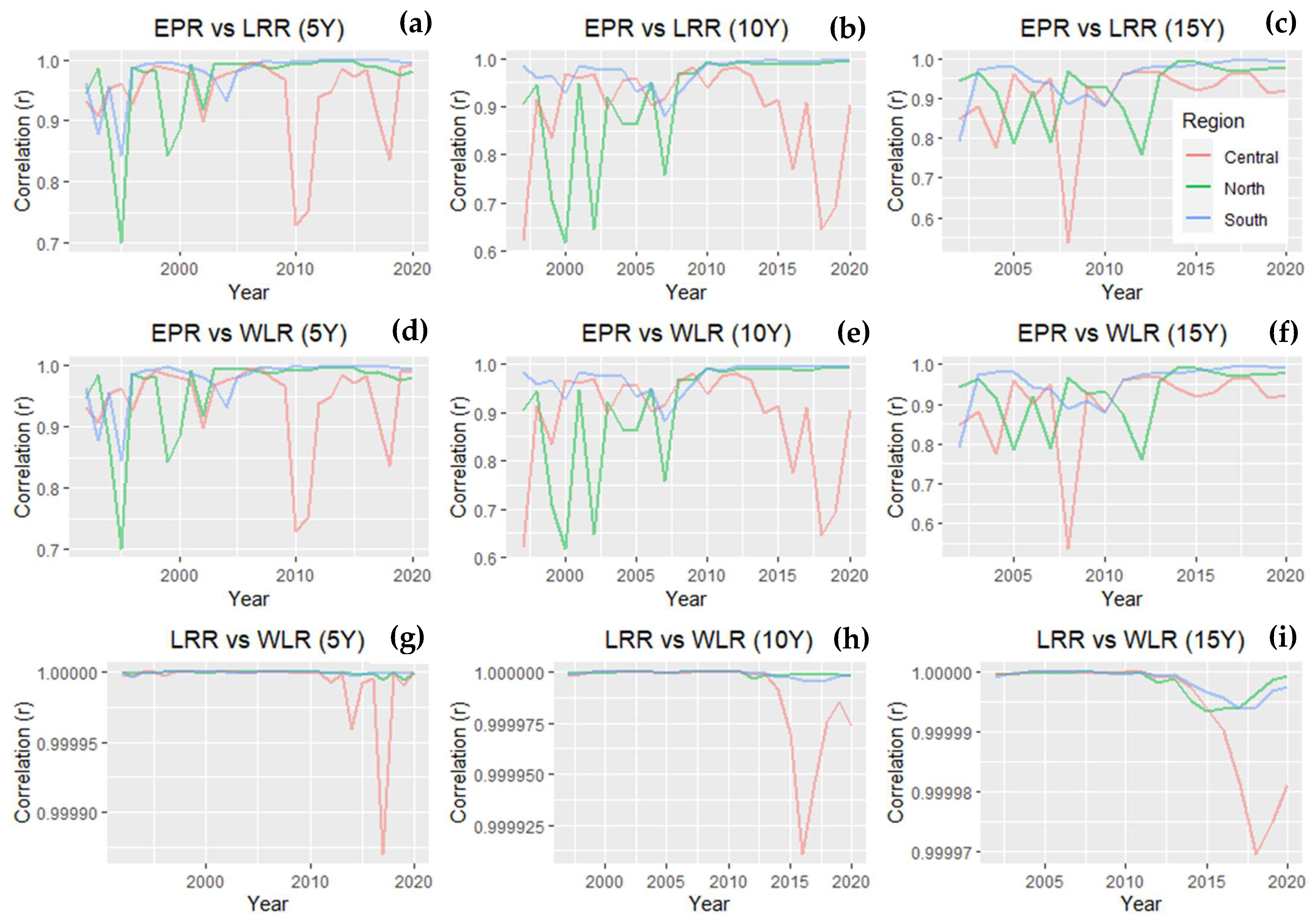
In this study, the EPR, LRR, and WLR methods were used to calculate shoreline change rates. Figure 3 reveals patterns of spatio-temporal correlation of shoreline rates between different methods used. Our results suggest that among the methods used, the LRR and WLR rates are highly positively correlated (>99%) for all time depths and regions. Since the LRR and WLR rates are highly correlated, a similar pattern of correlation between EPR vs. LRR and EPR vs. WLR were observed. Our analysis also suggests that correlation values varied over time and space. The correlation between EPR and LRR rates ranged from 0.7–1 (5 y time depth), 0.62–1 (10 y time depth), and 0.54–1 (15 y time depth). Most of the years, the correlation between the EPR and LRR were found to be strong (>0.7) for all regions, although a small number of observations had moderate (0.5–0.7) correlation values. These fluctuations in correlation values might be related to the way EPR and LRR rates are calculated. The EPR rates use only the beginning and end year shorelines while calculating the shoreline movement. On the other hand, the LRR rates use all the available shorelines to calculate shoreline change rates.
3.2. Spatio-Temporal Variation in Shoreline Change Rates
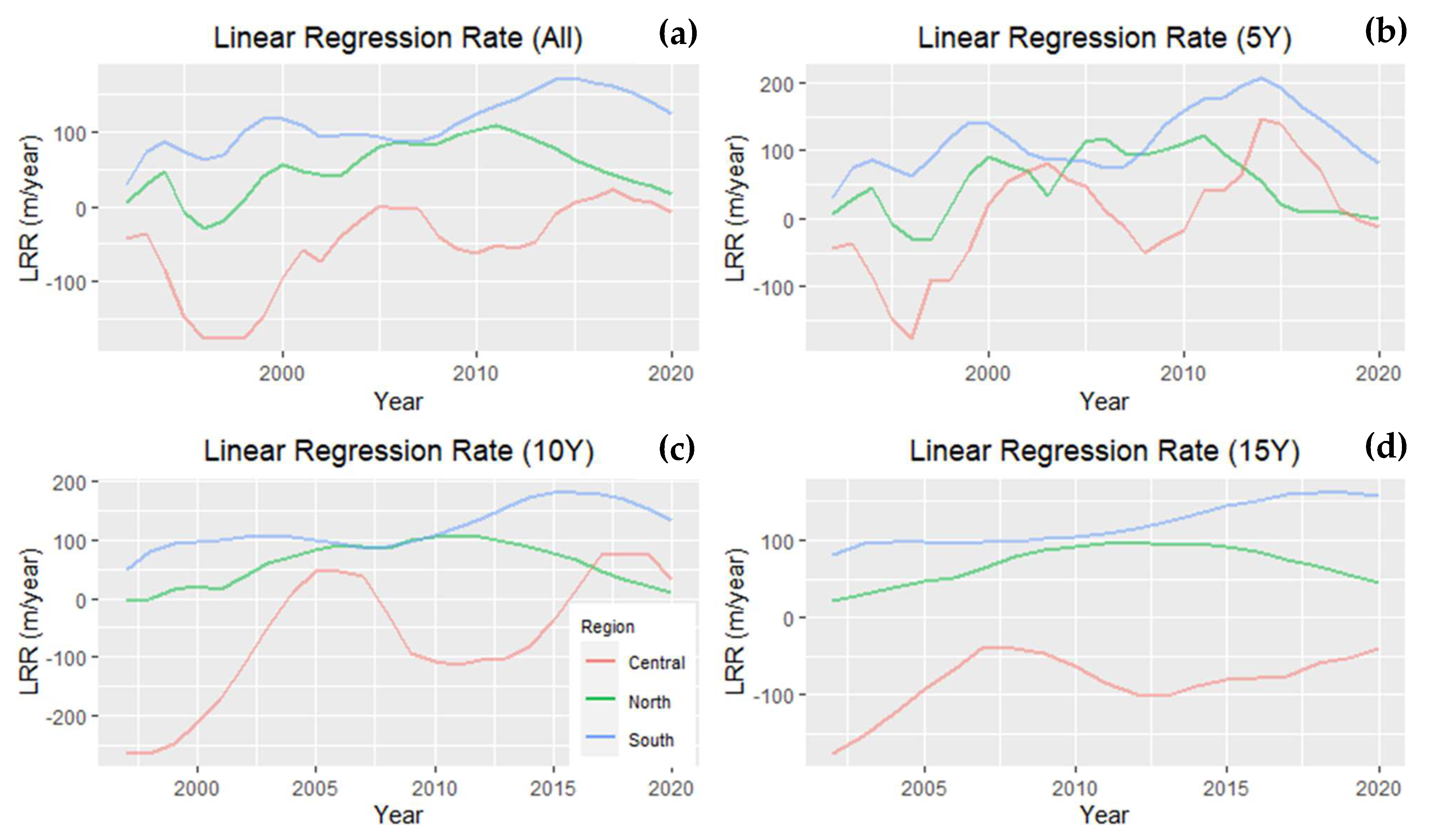
Figure 4 presents the LRR rates of shoreline movement over time and space. We present results calculated using the LRR rates but not the WLR rates due to the very high correlation of LRR and WLR. The LRR rates were also chosen over the WLR rates to align with the beta forecasting (Kalman filtering) used in the later part of the study to assess the prediction accuracy. Additionally, we excluded the EPR rates, since it only uses two specific shorelines to calculate the change rate. The LRR and WLR rates were found to be more sophisticated because they use all the shorelines available to calculate the rate.
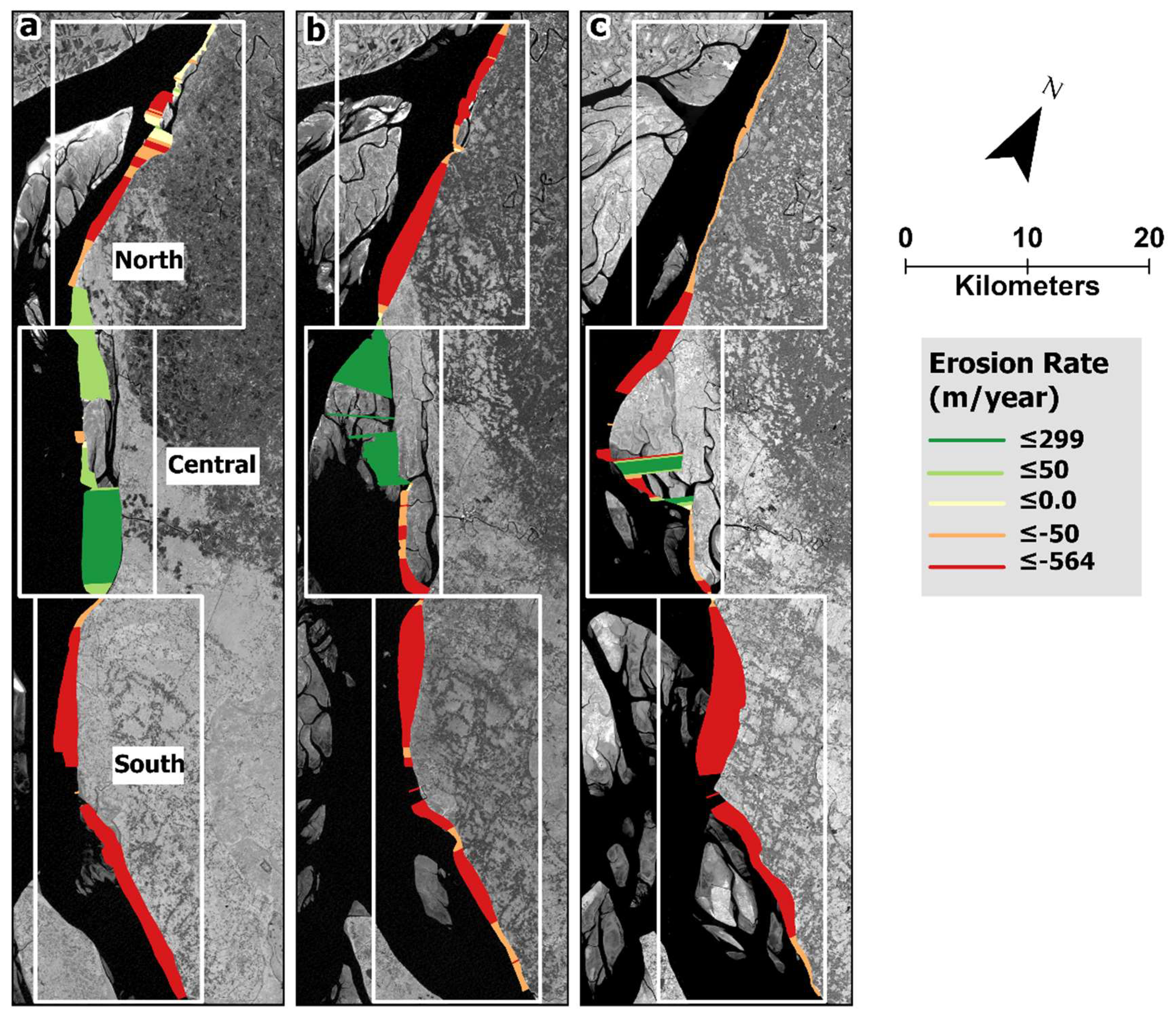
Among the regions, north and south region experienced primarily erosion while central region experienced mostly accretion over the studied period (1988–2021) (Figure 4; Appendix B). The LRR rates suggest that the central region experienced the highest average accretion rates (Figure 4a) in the years 1996–1998. During these years, average accretion rates were 177 m. On the other hand, the north and south regions experienced erosion most of the years. The highest rates of erosion were 109 m for the north region and 173 m for the south region in the years 2011 and 2015, respectively.
Among the time depths of data used, the distribution of the erosion/accretion rates suggest that the 15 years’ time depth data produced the lowest accretion/erosion rates for all regions compared to the 5 years and 10 years of data used in the model. This is likely due to the higher time depth smoothing out finer scale temporal variability compared to lower time depth. The highest rates of accretion (265 m) were found to be in the year 1998 when 10 years’ time depth data used. On the other hand, the highest rates of average erosion (207 m) were found to be in the year 2014 for 5 years’ time depth.
3.3. Spatio-Temporal Variation in Shoreline Prediction Performance
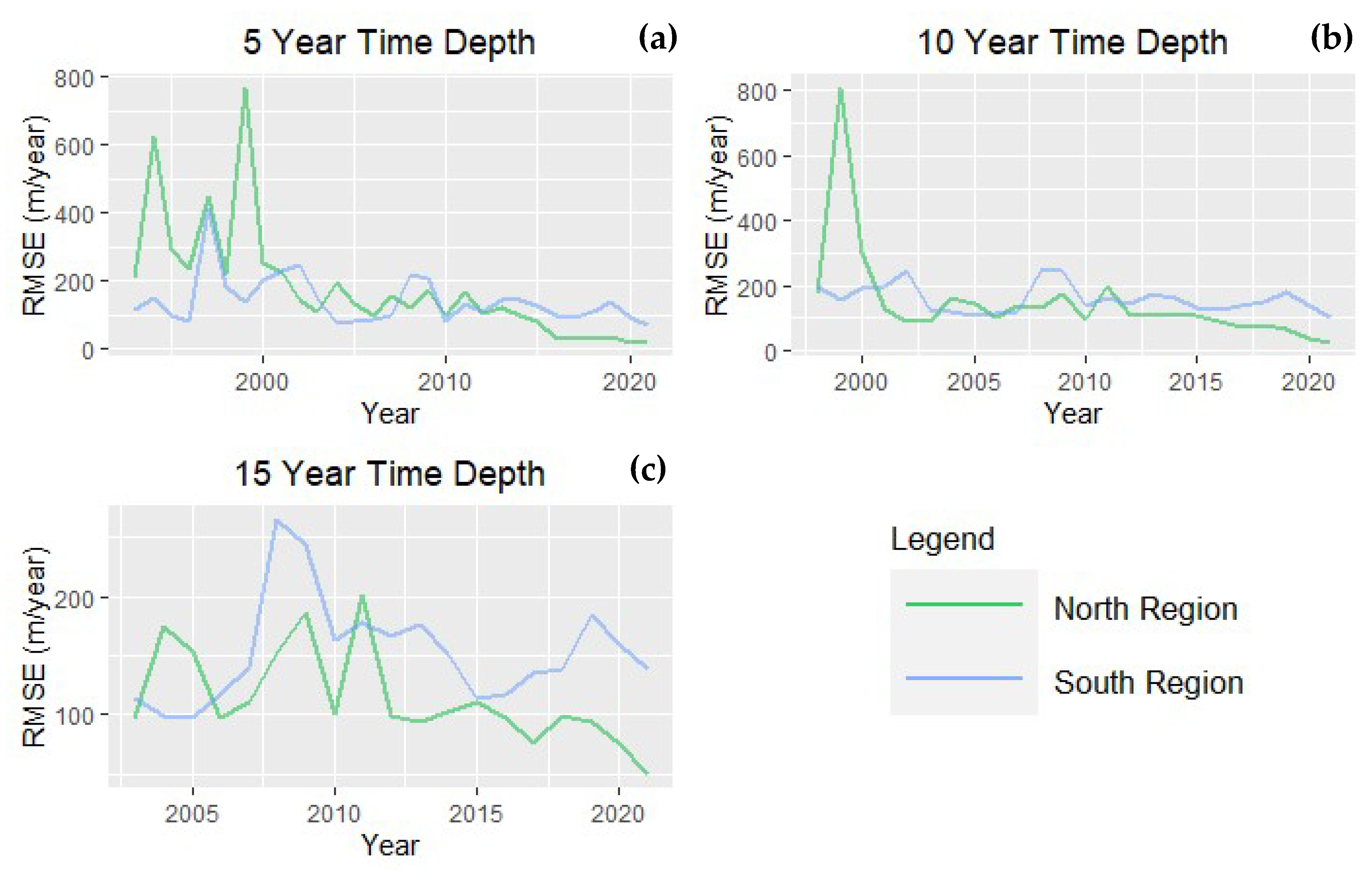
3.3.1. One-Year Shoreline Prediction Performance
Figure 5 reveals the spatio-temporal dynamics of 1-year prediction accuracy; e.g., predicting future shorelines one year into the future beyond a terminal date shoreline. The prediction accuracy of 1 year in the future was much better for the north and south regions compared to the central region. Our results suggest that among the regions studied, the RMSE values were lower in the recent years compared to the prior years for the north and south regions. On the other hand, the RMSE values fluctuated (62–2065 m) over time starting from the year 2007 for the central region. For this region, the prediction performed better in the prior years (before 2007) compared to the recent years. Due to the noisy nature of RMSE values for the different years in the central region, we have excluded the line showing the fluctuations in RMSE values. Removing the lines for central region in the plots (Figure 5) help in comparing with the RMSE values in the other figures.
In comparison of the RMSE values for different time depths used, this study found that the 5 years’ time depth data performed best in the south region while 10 and 15 years’ time depth data performed well in the north region. The average RMSE value was lowest (114 m) for the north region, while 15 years of time depth data used. The highest average RMSE values were found for the central regions, which can be explained due to the complex, noisy, and more highly variable nature of this region’s shoreline. The average RMSE values ranged from 556–640 m for this region. While combining the RMSE values for the different regions using all time depths, this study found that the north region had the lowest error (147 m) in predicting 1 year in the future. On the other hand, the highest RMSE value (585 m) was found for the central region.
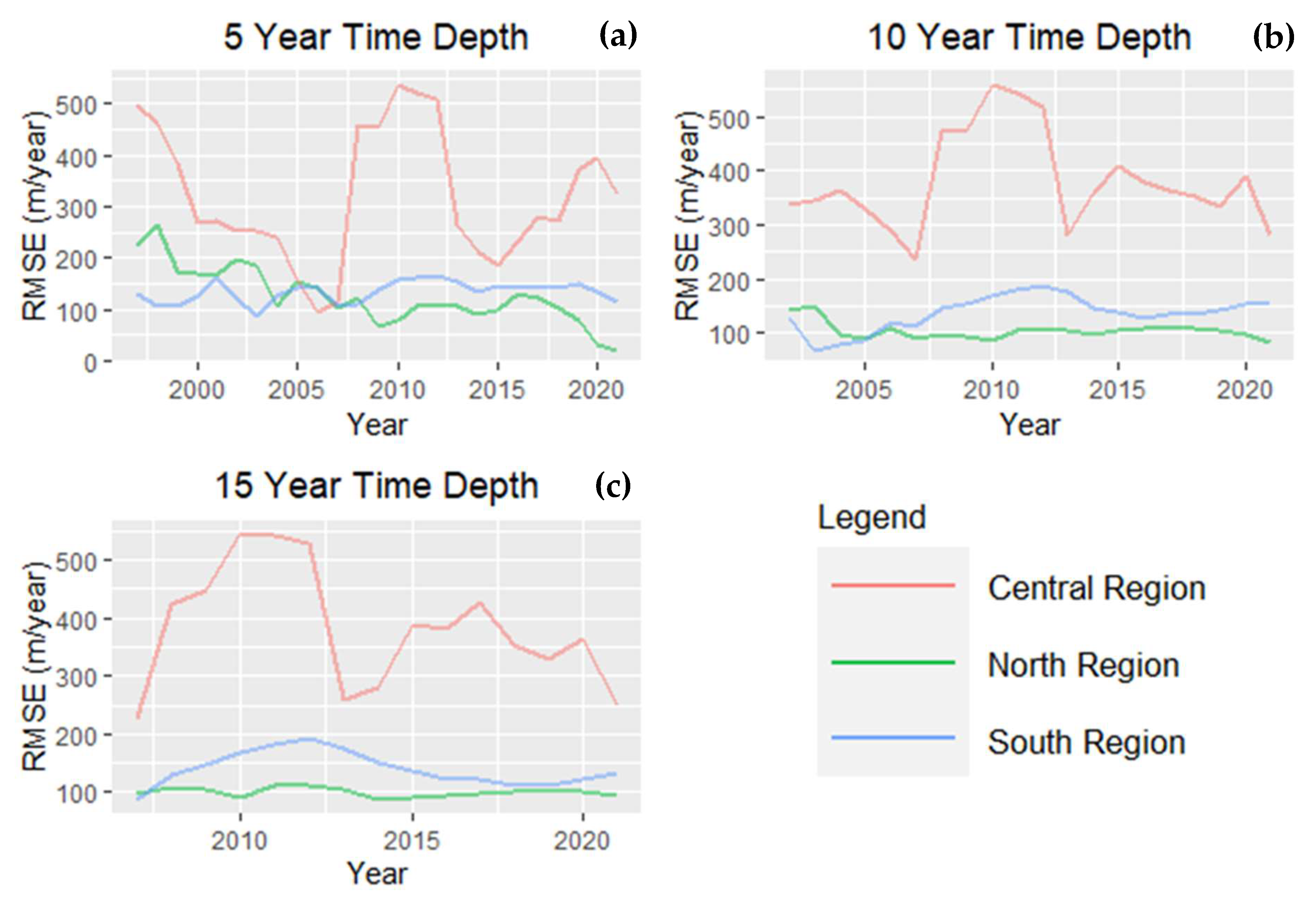
3.3.2. Five-Year Shoreline Prediction Performance
Similar to 1-year prediction, the LRR rates were utilized to predict shoreline positions 5 years into the future. Figure 6 illustrates the spatio-temporal pattern of the shoreline prediction performance using RMSE values. The prediction performance was again much better for the north and south regions compared to the central region for all different time depths used in this study. We believe that the RMSE values were much higher for the central region due to its complex nature and higher accretion rates over time.
We found that the north region had the lowest average RMSE value (111 m/year) over other the two regions followed by the south region (137 m/year) while combining all time depth data. The average RMSE value of different time depth data suggest that the north region had the lowest average RMSE value (101 m/year) using 15 years’ time depth. The aggregation of all regions’ RMSE values suggest that the lowest (194 m/year) and highest (208 m/year) values were found when 5 years’ and 15 years’ time depth data was used, respectively.
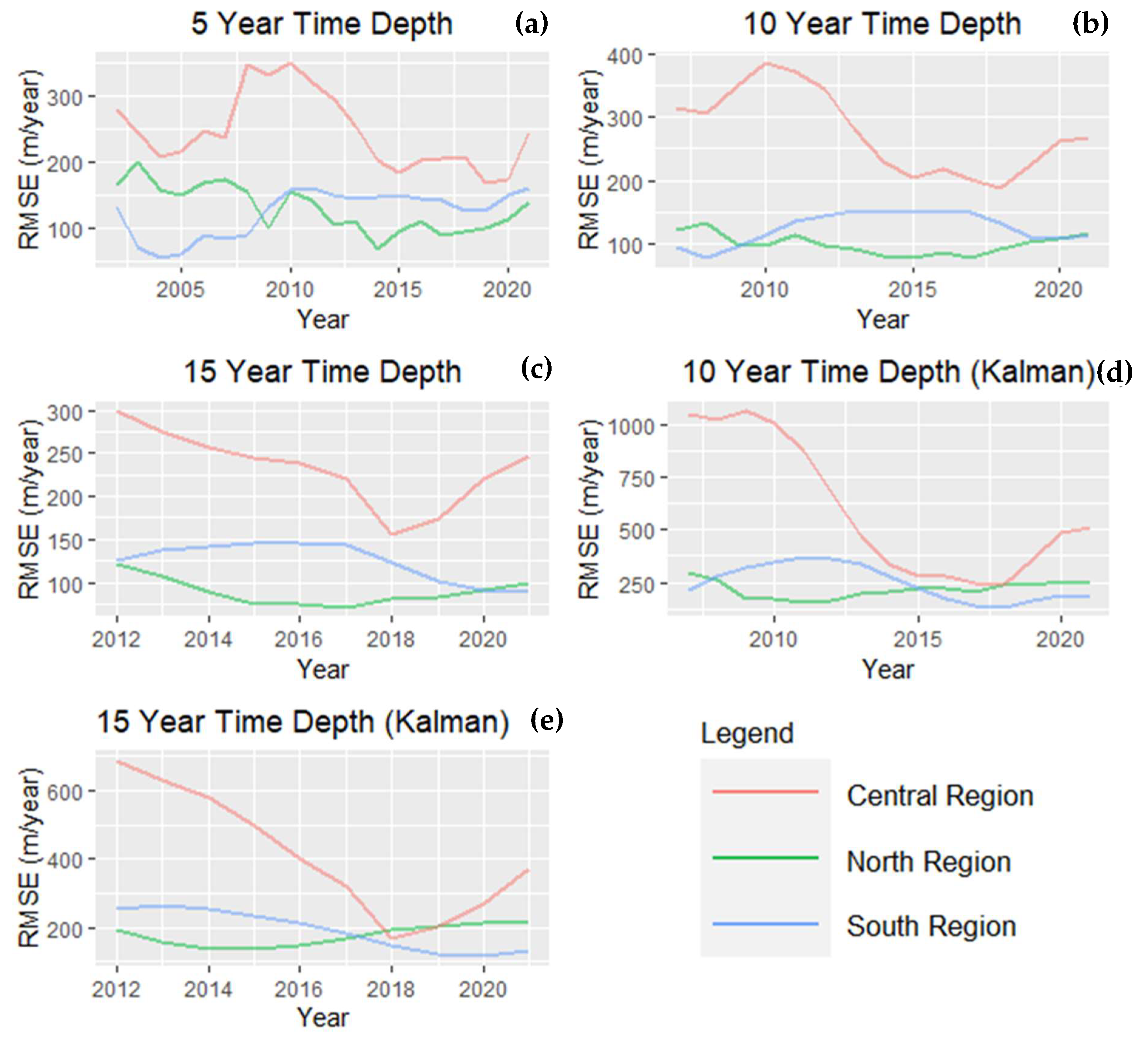
3.3.3. Ten-Year Shoreline Prediction Performance
Using normal extrapolation and the Kalman filter method, shoreline positions were predicted for 10 years into the future and accuracy was assessed for all regions and different time depths (Figure 7). Our results suggest that, irrespective of the methods and time depths of the data used, the north and south regions performed better in predicting future shoreline positions compared to the central region. As already mentioned in the previous sections, this might be due to the complex nature of the shoreline movement in the central region.
In comparison between the LRR rates and Kalman filter predictions, our analysis suggests that the LRR rates outperformed the Kalman filter method of prediction. The RMSE values were found to be much lower when the LRR rates were used in prediction. While using the LRR rates for all depths, the lowest average RMSE value was found to be 106 m/year for the north region, while the highest value was found to be 252 m/year for the south region. On the other hand, for the Kalman filter method, the lowest and highest average RMSE value was 197 m/year and 503 m/year for north and south region respectively.
In terms of time depths used, the prediction accuracy was found to be much higher for the increased number of shorelines used for both the LRR rates and the Kalman filter method. The lowest average RMSE value was found to be 149 and 260 m/year for the LRR rates and Kalman filter method while 15 years of shoreline data was used in the model. This clearly indicates that higher numbers of shorelines yield higher accuracies. Results also indicate that the simple extrapolation outperformed than the Kalman filter method.
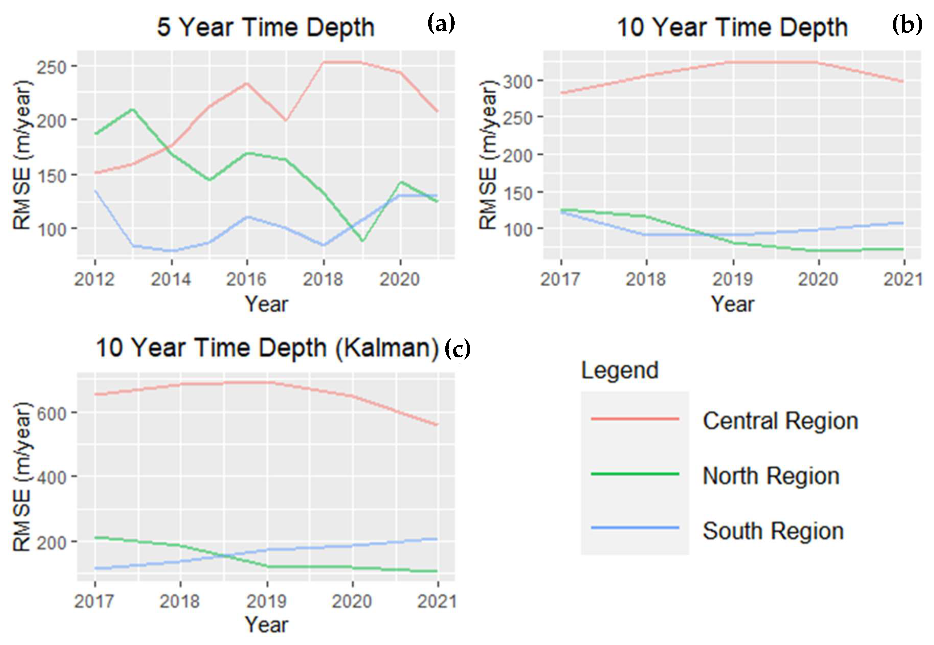
3.3.4. Twenty-Year Shoreline Prediction Performance
Figure 8 shows the spatio-temporal dynamics of shoreline prediction accuracy for 20 years in the future. Similar to the 10 years’ prediction, both the LRR rates and Kalman filtering methods were used to predict shoreline positions. Like 10 years prediction, simple extrapolation performed better than Kalman filter prediction. Results show that the average RMSE value of the LRR rates was 161 m/year while the value for Kalman filter method was 321 m/year.
Among the regions, and for the other different time horizons, the north and central regions performed better in predicting future shoreline positions. The average RMSE for the north, central, and south regions were found to be 123, 257, and 161 m/year, respectively, when the LRR rates were used. With the Kalman filter prediction, it was 150 m/year for the north, 647 m/year for the central, and 165 m/year for the south region.
The average RMSE value for 5 years’ time depth (156 m/year) were found to be the lowest among all depths used in predicting shorelines 20 years in the future. In comparison, between simple extrapolation and the Kalman filter prediction, it was found that the RMSE value was almost doubled for the Kalman method compared to the LRR rates. This result clearly suggests that the normal extrapolation outperformed the Kalman filter method in predicting 20 years into the future.
4. Discussion
In this study, the performance of future shoreline predictions was assessed using satellite imagery from 1988 to 2021. Approximately 85 km of the shoreline along the eastern bank of the lower Meghna River region in Bangladesh was used as the case in this study. The entire shoreline was divided into three zones based on their distinct rates of shoreline erosion and accretion. Previous research found that the north and south regions experienced extreme erosion over the last three decades, while the central region experienced dominant accretion [11,37], a finding we replicate here.
Our results suggest that the performance of shoreline predictions varied over time and space. It also varied by different methods used to predict future shoreline positions. The predictions performed best with relatively higher number of shorelines used as input to derive shoreline change rates. A clear finding is that higher time depth in estimating the shoreline change rates is preferable. Our analysis of RMSE for the prediction of future shoreline positions suggests that prediction performed better for the near future compared to distant. To come up with this conclusion, we compared the average RMSE values for the north and south regions (all time depths) of the 1 and 5 years (near future) to the mean of the 10 and 20 year values (distant future). Our results suggest that the average RMSE value for near future (138 m/year) was lower than the distant future (152 m/year). Thus, prediction for shorter time horizons is preferable, at least for this region and the statistical empirical methods employed. Among our study’s three defined regions, the north and south regions performed better in predicting future shoreline positions compared to the central region. This is understandable due to the complex and generally “noisy” form in terms of shoreline data mapping in the last decade in the central region of the study area. Our results also suggest that the simple extrapolation outperformed the Kalman filter method for the future shoreline prediction. The average RMSE values for simple extrapolation (128 m/year) were found to be much lower than the Kalman filter method (185 m/year).
Many studies have used DSAS to predict future shoreline positions. However, very few studies have assessed the performance of different methods used in predicting shoreline movement with the relatively rich temporal time series employed here. A recent study by Ciritci and Turk [21] used the DSAS model to compare the prediction accuracy of the Kalman filter and other statistical methods, such as the EPR, LRR, and WLR, using a future prediction time horizon of 10 and 20 years. They found that while using the Kalman filter method, the 10-year shoreline prediction provided a higher accuracy over the 20-year prediction. This result is aligned with our findings that the accuracy of the prediction is generally higher for the near future compared to the distant. They also found that among the EPR, LRR, and WLR methods, WLR provided more accurate results compared to the others. However, our finding suggests that the Kalman filter method underperformed compared to the simple extrapolation runs counter to prior findings. The possible reason behind this might be related to the nature of the shoreline and the severity and magnitude of the erosion rates in this region. Future research might analyze how the prediction performance varies over different regions with different shoreline change rates.
Compared to much of the coastal erosion literature, this work drew from a 34-year time series of satellite-derived shorelines at annual temporal resolution. This time depth enabled us to employ a temporal design strategy expected to yield a robust characterization of the space-time erosion patterns. It also enabled us to empirically assess the performance of future shoreline position predictions by quantifying how prediction performance varies depending on the time depths of the input historical shoreline data and the time horizons of predicted shorelines.
Though the location of this study is coastal Bangladesh, this is a methodological innovation with the potential for forecasting applications to other deltas and vulnerable shorelines globally. While empirical results are specific to the project’s study area, results can inform the region’s shoreline forecasting ability and the associated mitigation and adaptation strategies. This study also has implications in better planning and management of the lower Meghna River region of Bangladesh.
This study used the empirical data derived from satellite imagery to predict future shoreline positions. However, shorelines are heavily influenced by sediment transportation, local rainfall and floods, cyclones, and sea level rise. It is predicted that due to global warming and the resultant sea level rise, coastal erosion will increase in the future [38]. Since this study did not consider these influences in predicting future shoreline positions, this study has limitations. Further study is needed to consider the influence of the above-mentioned factors and to engage more deeply with comparison of the simple extrapolation method vs. the Kalman filter method for predicting future shorelines. While the empirical predictive methods used in this study may not be able to account for the physically process-based factors contributing to coastal erosion and accretion, they may be useful to inform both local residents and policy makers to plan of future impacts of shoreline change [39].
Due to the extreme rates of shoreline change in this region, we believe the errors are seen to be generally larger than the other similar studies around the world. Due to high errors, this kind of method might not be well suited to predicting shorelines in this region. However, we found that the error was much lower for the northern and southern regions compared to the central region. Further studies might need to assess how the prediction performance varies based on the shoreline change rates. A study on the Puri Coast of India by Mukhopadhyay et al. [40] found that the RMSE value to be 51.34 m when EPR rates were used. However, they didn’t mention the actual rate of erosion. Another study in the same coast found that the mean erosion rate was 16.33 m/year during 1990–2015 [41]. This indicates that the RMSE value was much higher for this coast compared to the actual erosion rates. It might be related to the long-term prediction of the coastal shoreline movement. As such, we suggest predicting for the near future (e.g., 1 year, 5 years) due to the high error in future shoreline prediction.
The tools used in this study do come with limitations. The DSAS tool used for future shoreline positions may not be ideal for all data types, locations and patterns of shoreline change [22,29]. Future researchers and those in applied practice should be cognizant of the methodological limitations when using competing shoreline change rates and future shoreline prediction models. A clear message and contribution of this work is that shoreline change rates and the resulting future shoreline positional prediction can vary depending on: (1) choice of change rate used, (2) choice of time depth used to derive change rates, (3) choice of time horizon for predicting future shorelines, (4) the time period in which rates are derived and future shoreline positions are predicted, and (5) the regional locations for which rates, predictions, and time periods are employed. In conclusion, both methodological considerations of rates and prediction methods along with considerations of time and space variability must be considered.
5. Conclusions
This study was carried out to assess the performance of empirical forecasting of future shoreline positions. To do so, this study used the eastern bank of the lower Meghna River in Bangladesh as the case site. This area is well evident to be one of the most erosion-prone areas in the world. This study adopted a data-driven approach to predict future shoreline positions using various statistical methods by examining past shoreline change rates at a 95% confidence interval (CI). Using different time depths of shoreline rates, methods of erosion rate calculation, and predicting future shoreline positions for different time horizons, this study assessed the prediction performance of different combinations. This study concludes that the higher the number of shorelines used in calculating and predicting shoreline the better the performance is. It was revealed that the prediction accuracy is generally higher for the near future (138 m/year) compared to the distant future (152 m/year). Our results also suggest that the normal extrapolation method (128 m/year) of prediction outperformed the Kalman filter method (185 m/year) in predicting future shoreline positions. However, it is important to determine the historical change rates and predict future shoreline positions for the long-term planning and management of coastal areas. It is critically important because future climate change is likely to exacerbate coastal erosion globally.
Author Contributions
Conceptualization, M.S.I. and T.W.C.; methodology, M.S.I. and T.W.C.; software, M.S.I.; validation, T.W.C.; formal analysis, M.S.I.; data curation, M.S.I. and T.W.C.; writing—original draft preparation, M.S.I.; writing—review and editing, M.S.I. and T.W.C.; visualization, M.S.I.; supervision, T.W.C.; funding acquisition, T.W.C. All authors have read and agreed to the published version of the manuscript.
Funding
This research was funded by the U.S. National Science Foundation, grant number 1660447.
Acknowledgments
We would like to thank Munshi Khaledur Rahman for his contribution in generating shorelines for the initial years while working as a postdoctoral researcher in this project.
Conflicts of Interest
The authors declare no conflict of interest.
Appendix A

Table A1.
Datasets used in the study.
| Image Date | Representative Year | Satellite | Path/Row | Resolution (m) |
|---|---|---|---|---|
| 19 February 1988 | 1988 | Landsat 5 | 137/44 | 30 |
| 21 February 1989 | 1989 | Landsat 5 | 137/44 | 30 |
| 7 January 1990 | 1990 | Landsat 5 | 137/44 | 30 |
| 15 March 1991 | 1991 | Landsat 5 | 137/44 | 30 |
| 12 December 1991 | 1992 | Landsat 5 | 137/44 | 30 |
| 30 December 1992 | 1993 | Landsat 5 | 137/44 | 30 |
| 2 January 1994 | 1994 | Landsat 5 | 137/44 | 30 |
| 21 January 1995 | 1995 | Landsat 5 | 137/44 | 30 |
| 9 February 1996 | 1996 | Landsat 5 | 137/44 | 30 |
| 26 January 1997 | 1997 | Landsat 5 | 137/44 | 30 |
| 14 February 1998 | 1998 | Landsat 5 | 137/44 | 30 |
| 17 February 1999 | 1999 | Landsat 5 | 137/44 | 30 |
| 20 February 2000 | 2000 | Landsat 5 | 137/44 | 30 |
| 5 January 2001 | 2001 | Landsat 5 | 137/44 | 30 |
| 1 February 2002 | 2002 | Landsat 7 | 137/44 | 30 |
| 2 December 2002 | 2003 | Landsat 7 | 137/44 | 30 |
| 13 December 2003 | 2004 | Landsat 5 | 137/44 | 30 |
| 15 December 2004 | 2005 | Landsat 5 | 137/44 | 30 |
| 4 February 2006 | 2006 | Landsat 5 | 137/44 | 30 |
| 22 January 2007 | 2007 | Landsat 5 | 137/44 | 30 |
| 16 December 2007 | 2008 | Landsat 7 | 137/44 | 30 |
| 3 January 2009 | 2009 | Landsat 7 | 137/44 | 30 |
| 30 January 2010 | 2010 | Landsat 5 | 137/44 | 30 |
| 1 January 2011 | 2011 | Landsat 5 | 137/44 | 30 |
| 28 January 2012 | 2012 | Landsat 7 | 137/44 | 30 |
| 14 January 2013 | 2013 | Landsat 7 | 137/44 | 30 |
| 24 December 2013 | 2014 | Landsat 8 | 137/44 | 30 |
| 25 November 2014 | 2015 | Landsat 8 | 137/44 | 30 |
| 30 December 2015 | 2016 | Landsat 8 | 137/44 | 30 |
| 1 January 2017 | 2017 | Landsat 8 | 137/44 | 30 |
| 4 January 2018 | 2018 | Landsat 8 | 137/44 | 30 |
| 7 January 2019 | 2019 | Landsat 8 | 137/44 | 30 |
| 10 January 2020 | 2020 | Landsat 8 | 137/44 | 30 |
| 27 December 2020 | 2021 | Landsat 8 | 137/44 | 30 |
Appendix B
Figure A1.
Decadal shoreline movement in the eastern bank of the lower Meghna River region in Bangladesh: (a) 1990–1999, (b) 2000–2009, (c) 2010–2019. In the map, positive values indicate accretion and negative values indicate erosion.
Figure A1.
Decadal shoreline movement in the eastern bank of the lower Meghna River region in Bangladesh: (a) 1990–1999, (b) 2000–2009, (c) 2010–2019. In the map, positive values indicate accretion and negative values indicate erosion.

References
- Sahoo, B.; Bhaskaran, P.K. Multi-Hazard Risk Assessment of Coastal Vulnerability from Tropical Cyclones—A GIS Based Approach for the Odisha Coast. J. Environ. Manag. 2018, 206, 1166–1178. [Google Scholar] [CrossRef] [PubMed]
- UN. Factsheet: People and Oceans; United Nations: New York, NY, USA, 2017. [Google Scholar]
- Klein, R.J.T.; Nicholls, R.J.; Thomalla, F. Resilience to Natural Hazards: How Useful Is This Concept? Environ. Hazards 2003, 5, 35–45. [Google Scholar] [CrossRef]
- Passeri, D.L.; Hagen, S.C.; Medeiros, S.C.; Bilskie, M.V.; Alizad, K.; Wang, D. The Dynamic Effects of Sea Level Rise on Low-Gradient Coastal Landscapes: A Review. Earth’s Future 2015, 3, 159–181. [Google Scholar] [CrossRef]
- Woodroffe, C.D.; Nicholls, R.J.; Saito, Y.; Chen, Z.; Goodbred, S.L. Landscape Variability and the Response of Asian Megadeltas to Environmental Change. In Global Change and Integrated Coastal Management: The Asia-Pacific Region; Coastal Systems and Continental Margins; Harvey, N., Ed.; Springer: Dordrecht, The Netherlands, 2006; pp. 277–314. ISBN 978-1-4020-3628-6. [Google Scholar]
- Dangendorf, S.; Marcos, M.; Wöppelmann, G.; Conrad, C.P.; Frederikse, T.; Riva, R. Reassessment of 20th Century Global Mean Sea Level Rise. Proc. Natl. Acad. Sci. USA 2017, 114, 5946–5951. [Google Scholar] [CrossRef] [PubMed] [Green Version]
- Hay, C.C.; Morrow, E.; Kopp, R.E.; Mitrovica, J.X. Probabilistic Reanalysis of Twentieth-Century Sea-Level Rise. Nature 2015, 517, 481–484. [Google Scholar] [CrossRef]
- Zhang, K.; Douglas, B.C.; Leatherman, S.P. Global Warming and Coastal Erosion. Clim. Chang. 2004, 64, 41. [Google Scholar] [CrossRef]
- Brammer, H. Bangladesh’s Dynamic Coastal Regions and Sea-Level Rise. Clim. Risk Manag. 2014, 1, 51–62. [Google Scholar] [CrossRef] [Green Version]
- Ahmed, A.; Drake, F.; Nawaz, R.; Woulds, C. Where Is the Coast? Monitoring Coastal Land Dynamics in Bangladesh: An Integrated Management Approach Using GIS and Remote Sensing Techniques. Ocean Coast. Manag. 2018, 151, 10–24. [Google Scholar] [CrossRef]
- Crawford, T.W.; Rahman, M.K.; Miah, M.G.; Islam, M.R.; Paul, B.K.; Curtis, S.; Islam, M.S. Coupled Adaptive Cycles of Shoreline Change and Households in Deltaic Bangladesh: Analysis of a 30-Year Shoreline Change Record and Recent Population Impacts. Ann. Am. Assoc. Geogr. 2021, 111, 1002–1024. [Google Scholar] [CrossRef]
- Crawford, T.W.; Islam, M.S.; Rahman, M.K.; Paul, B.K.; Curtis, S.; Miah, M.G.; Islam, M.R. Coastal Erosion and Human Perceptions of Revetment Protection in the Lower Meghna Estuary of Bangladesh. Remote Sens. 2020, 12, 3108. [Google Scholar] [CrossRef]
- Paul, B.K.; Rahman, M.K.; Crawford, T.; Curtis, S.; Miah, M.G.; Islam, M.R.; Islam, M.S. Explaining Mobility Using the Community Capital Framework and Place Attachment Concepts: A Case Study of Riverbank Erosion in the Lower Meghna Estuary, Bangladesh. Appl. Geogr. 2020, 125, 102199. [Google Scholar] [CrossRef]
- Hossain, M.S.; Dearing, J.A.; Rahman, M.M.; Salehin, M. Recent Changes in Ecosystem Services and Human Well-Being in the Bangladesh Coastal Zone. Reg. Environ. Chang. 2016, 16, 429–443. [Google Scholar] [CrossRef] [Green Version]
- Poncelet, A.; Gemenne, F.; Martiniello, M.; Bousetta, H. A Country Made for Disasters: Environmental Vulnerability and Forced Migration in Bangladesh. In Environment, Forced Migration and Social Vulnerability; Afifi, T., Jäger, J., Eds.; Springer: Berlin/Heidelberg, Germany, 2010; pp. 211–222. ISBN 978-3-642-12416-7. [Google Scholar]
- Splinter, K.D.; Coco, G. Challenges and Opportunities in Coastal Shoreline Prediction. Front. Mar. Sci. 2021, 8, 788657. [Google Scholar] [CrossRef]
- Bamunawala, J.; Ranasinghe, R.; Dastgheib, A.; Nicholls, R.J.; Murray, A.B.; Barnard, P.L.; Sirisena, T.A.J.G.; Duong, T.M.; Hulscher, S.J.M.H.; van der Spek, A. Twenty-First-Century Projections of Shoreline Change along Inlet-Interrupted Coastlines. Sci. Rep. 2021, 11, 14038. [Google Scholar] [CrossRef]
- Sanuy, M.; Jiménez, J.A. Sensitivity of Storm-Induced Hazards in a Highly Curvilinear Coastline to Changing Storm Directions. The Tordera Delta Case (NW Mediterranean). Water 2019, 11, 747. [Google Scholar] [CrossRef] [Green Version]
- Ibaceta, R.; Splinter, K.D.; Harley, M.D.; Turner, I.L. Enhanced Coastal Shoreline Modeling Using an Ensemble Kalman Filter to Include Nonstationarity in Future Wave Climates. Geophys. Res. Lett. 2020, 47, e2020GL090724. [Google Scholar] [CrossRef]
- Vitousek, S.; Barnard, P.L.; Limber, P.; Erikson, L.; Cole, B. A Model Integrating Longshore and Cross-Shore Processes for Predicting Long-Term Shoreline Response to Climate Change. J. Geophys. Res. Earth Surf. 2017, 122, 782–806. [Google Scholar] [CrossRef]
- Ciritci, D.; Türk, T. Assessment of the Kalman Filter-Based Future Shoreline Prediction Method. Int. J. Environ. Sci. Technol. 2020, 17, 3801–3816. [Google Scholar] [CrossRef]
- Yan, D.; Yao, X.; Li, J.; Qi, L.; Luan, Z. Shoreline Change Detection and Forecast along the Yancheng Coast Using a Digital Shoreline Analysis System. Wetlands 2021, 41, 47. [Google Scholar] [CrossRef]
- Sarwar, M.G.M.; Woodroffe, C.D. Rates of Shoreline Change along the Coast of Bangladesh. J. Coast Conserv. 2013, 17, 515–526. [Google Scholar] [CrossRef]
- Kaliraj, S.; Chandrasekar, N.; Ramachandran, K.K.; Srinivas, Y.; Saravanan, S. Coastal Landuse and Land Cover Change and Transformations of Kanyakumari Coast, India Using Remote Sensing and GIS. Egypt. J. Remote Sens. Space Sci. 2017, 20, 169–185. [Google Scholar] [CrossRef]
- Thieler, E.R.; Himmelstoss, E.A.; Zichichi, J.L.; Ergul, A. The Digital Shoreline Analysis System (DSAS) Version 4.0—An ArcGIS Extension for Calculating Shoreline Change; Open-File Report; U.S. Geological Survey: Reston, VA, USA, 2009; Volume 2008-1278.
- Mondal, I.; Thakur, S.; Juliev, M.; Bandyopadhyay, J.; De, T.K. Spatio-Temporal Modelling of Shoreline Migration in Sagar Island, West Bengal, India. J. Coast Conserv. 2020, 24, 50. [Google Scholar] [CrossRef]
- Patel, K.; Jain, R.; Patel, A.N.; Kalubarme, M.H. Shoreline Change Monitoring for Coastal Zone Management Using Multi-Temporal Landsat Data in Mahi River Estuary, Gujarat State. Appl. Geomat. 2021, 13, 333–347. [Google Scholar] [CrossRef]
- Al-Zubieri, A.G.; Ghandour, I.M.; Bantan, R.A.; Basaham, A.S. Shoreline Evolution Between Al Lith and Ras Mahāsin on the Red Sea Coast, Saudi Arabia Using GIS and DSAS Techniques. J. Indian Soc. Remote Sens. 2020, 48, 1455–1470. [Google Scholar] [CrossRef]
- Himmelstoss, E.A.; Henderson, R.E.; Kratzmann, M.G.; Farris, A.S. Digital Shoreline Analysis System (DSAS) Version 5.0 User Guide; Open-File Report; U.S. Geological Survey: Reston, VA, USA, 2018; Volume 2018-1179.
- Paul, B.K.; Rahman, M.K.; Crawford, T.; Curtis, S.; Miah, M.G.; Islam, R.; Islam, M.S. Coping Strategies of People Displaced by Riverbank Erosion in the Lower Meghna Estuary. In Living on the Edge: Char Dwellers in Bangladesh; Springer Geography; Zaman, M., Alam, M., Eds.; Springer International Publishing: Cham, Switzerland, 2021; pp. 227–239. ISBN 978-3-030-73592-0. [Google Scholar]
- Rahman, M.K.; Crawford, T.W.; Paul, B.K.; Islam, M.S.; Curtis, S.; Miah, M.G.; Islam, M.R. Riverbank Erosions, Coping Strategies, and Resilience Thinking of the Lower-Meghna River Basin Community, Bangladesh. In Climate Vulnerability and Resilience in the Global South: Human Adaptations for Sustainable Futures; Climate Change Management; Alam, G.M.M., Erdiaw-Kwasie, M.O., Nagy, G.J., Filho, W.L., Eds.; Springer International Publishing: Cham, Switzerland, 2021; pp. 259–278. ISBN 978-3-030-77259-8. [Google Scholar]
- Ghoneim, E.; Mashaly, J.; Gamble, D.; Halls, J.; AbuBakr, M. Nile Delta Exhibited a Spatial Reversal in the Rates of Shoreline Retreat on the Rosetta Promontory Comparing Pre- and Post-Beach Protection. Geomorphology 2015, 228, 1–14. [Google Scholar] [CrossRef]
- Luijendijk, A.; Hagenaars, G.; Ranasinghe, R.; Baart, F.; Donchyts, G.; Aarninkhof, S. The State of the World’s Beaches. Sci. Rep. 2018, 8, 6641. [Google Scholar] [CrossRef]
- Xu, H. Modification of Normalised Difference Water Index (NDWI) to Enhance Open Water Features in Remotely Sensed Imagery. Int. J. Remote Sens. 2006, 27, 3025–3033. [Google Scholar] [CrossRef]
- Hapke, C.; Himmelstoss, E.; Kratzmann, M.; Thieler, E. National Assessment of Shoreline Change: Historical Shoreline Change along the New England and Mid-Atlantic Coasts; U.S. Geological Survey: Reston, VA, USA, 2011.
- Mullick, M.R.A.; Islam, K.M.A.; Tanim, A.H. Shoreline Change Assessment Using Geospatial Tools: A Study on the Ganges Deltaic Coast of Bangladesh. Earth Sci. Inform. 2020, 13, 299–316. [Google Scholar] [CrossRef]
- Mahmud, M.I.; Mia, A.J.; Islam, M.A.; Peas, M.H.; Farazi, A.H.; Akhter, S.H. Assessing Bank Dynamics of the Lower Meghna River in Bangladesh: An Integrated GIS-DSAS Approach. Arab. J. Geosci. 2020, 13, 602. [Google Scholar] [CrossRef]
- Vousdoukas, M.I.; Ranasinghe, R.; Mentaschi, L.; Plomaritis, T.A.; Athanasiou, P.; Luijendijk, A.; Feyen, L. Sandy Coastlines under Threat of Erosion. Nat. Clim. Chang. 2020, 10, 260–263. [Google Scholar] [CrossRef]
- Agrawal, G.; Ferhatosmanoglu, H.; Niu, X.; Bedford, K.; Li, R. A Vision for Cyberinfrastructure for Coastal Forecasting and Change Analysis. In GeoSensor Networks: Second International Conference, GSN 2006, Boston, MA, USA, October 1–3, 2006, Revised Selected and Invited Papers; Lecture Notes in Computer Science; Nittel, S., Labrinidis, A., Stefanidis, A., Eds.; Springer: Berlin/Heidelberg, Germany, 2008; pp. 151–174. ISBN 978-3-540-79996-2. [Google Scholar]
- Mukhopadhyay, A.; Mukherjee, S.; Mukherjee, S.; Ghosh, S.; Hazra, S.; Mitra, D. Automatic Shoreline Detection and Future Prediction: A Case Study on Puri Coast, Bay of Bengal, India. Eur. J. Remote Sens. 2012, 45, 201–213. [Google Scholar] [CrossRef]
- Mukhopadhyay, A.; Ghosh, P.; Chanda, A.; Ghosh, A.; Ghosh, S.; Das, S.; Ghosh, T.; Hazra, S. Threats to Coastal Communities of Mahanadi Delta Due to Imminent Consequences of Erosion—Present and near Future. Sci. Total Environ. 2018, 637–638, 717–729. [Google Scholar] [CrossRef] [PubMed]
Figure 1.
Study area—the eastern bank of lower Meghna River region in Bangladesh.

Figure 2.
Flowchart of the methodology followed to conduct this study.

Figure 3.
Spatio-temporal pattern of the Pearson correlation (r) values between different methods used to calculate historical shoreline change rates: (a) 5 years’ time depth EPR vs. LRR, (b) 10 years’ time depth EPR vs. LRR, (c) 15 years’ time depth EPR vs. LRR, (d) 5 years’ time depth EPR vs. WLR, (e) 10 years’ time depth EPR vs. WLR, (f) 15 years’ time depth EPR vs. WLR, (g) 5 years’ time depth LRR vs. WLR, (h) 10 years’ time depth LRR vs. WLR, and (i) 15 years’ time depth LRR vs. WLR.

Figure 4.
Linear regression rate of shoreline movement over time and space: (a) average of all time depths, (b) 5 years’ time depth, (c) 10 years’ time depth, and (d) 15 years’ time depth. In the figure, positive values indicate erosion and negative values indicate accretion.
Figure 4.
Linear regression rate of shoreline movement over time and space: (a) average of all time depths, (b) 5 years’ time depth, (c) 10 years’ time depth, and (d) 15 years’ time depth. In the figure, positive values indicate erosion and negative values indicate accretion.

Figure 5.
Variations in RMSE values calculated using the LRR rates data for predicting 1 year in the future: (a) 5 years’ time depth, (b) 10 years’ time depth, and (c) 15 years’ time depth.
Figure 5.
Variations in RMSE values calculated using the LRR rates data for predicting 1 year in the future: (a) 5 years’ time depth, (b) 10 years’ time depth, and (c) 15 years’ time depth.

Figure 6.
Variations in RMSE values calculated using the LRR rates data for predicting 5 years in the future: (a) 5 years’ time depth, (b) 10 years’ time depth, and (c) 15 years’ time depth.
Figure 6.
Variations in RMSE values calculated using the LRR rates data for predicting 5 years in the future: (a) 5 years’ time depth, (b) 10 years’ time depth, and (c) 15 years’ time depth.

Figure 7.
Variations in RMSE values of the LRR rates in predicting 10 years in the future calculated: (a) 5 years’ time depth, (b) 10 years’ time depth, (c) 15 years’ time depth, (d) 10 years’ time depth (Kalman), and (e) 15 years’ time depth (Kalman).
Figure 7.
Variations in RMSE values of the LRR rates in predicting 10 years in the future calculated: (a) 5 years’ time depth, (b) 10 years’ time depth, (c) 15 years’ time depth, (d) 10 years’ time depth (Kalman), and (e) 15 years’ time depth (Kalman).

Figure 8.
Variations in RMSE values calculated using the LRR rates data for predicting 20 years in the future: (a) 5 years’ time depth, (b) 10 years’ time depth, and (c) 10 years’ time depth (Kalman).
Figure 8.
Variations in RMSE values calculated using the LRR rates data for predicting 20 years in the future: (a) 5 years’ time depth, (b) 10 years’ time depth, and (c) 10 years’ time depth (Kalman).

Table 1.
Summary statistics of different parameters used in shoreline uncertainty assessment.
| Georeferencing Uncertainty (Ug) | Pixel Uncertainty (Up) | Digitizing Uncertainty (Ud) | Tidal Uncertainty (Ut) | Total Uncertainty (Utotal) | |
|---|---|---|---|---|---|
| Minimum | 3.54 | 30 | 0 | 5.60 | 30.72 |
| Maximum | 7.34 | 30 | 0 | 19.60 | 36.58 |
| Mean | 4.72 | 30 | 0 | 7.32 | 32.27 |
All units are in meters.
Publisher’s Note: MDPI stays neutral with regard to jurisdictional claims in published maps and institutional affiliations. |
© 2022 by the authors. Licensee MDPI, Basel, Switzerland. This article is an open access article distributed under the terms and conditions of the Creative Commons Attribution (CC BY) license (https://creativecommons.org/licenses/by/4.0/).
Share and Cite
MDPI and ACS Style
Islam, M.S.; Crawford, T.W. Assessment of Spatio-Temporal Empirical Forecasting Performance of Future Shoreline Positions. Remote Sens. 2022, 14, 6364. https://0-doi-org.brum.beds.ac.uk/10.3390/rs14246364
AMA Style
Islam MS, Crawford TW. Assessment of Spatio-Temporal Empirical Forecasting Performance of Future Shoreline Positions. Remote Sensing. 2022; 14(24):6364. https://0-doi-org.brum.beds.ac.uk/10.3390/rs14246364
Chicago/Turabian StyleIslam, Md Sariful, and Thomas W. Crawford. 2022. "Assessment of Spatio-Temporal Empirical Forecasting Performance of Future Shoreline Positions" Remote Sensing 14, no. 24: 6364. https://0-doi-org.brum.beds.ac.uk/10.3390/rs14246364
Note that from the first issue of 2016, this journal uses article numbers instead of page numbers. See further details here.