Article

Machine-Learning Classification of SAR Remotely-Sensed Sea-Surface Petroleum Signatures—Part 1: Training and Testing Cross Validation

by
Gustavo de Araújo Carvalho
1,*,
Peter J. Minnett
2,
Nelson F. F. Ebecken
3 and
Luiz Landau
1
1
Laboratório de Sensoriamento Remoto por Radar Aplicado à Indústria do Petróleo (LabSAR), Laboratório de Métodos Computacionais em Engenharia (LAMCE), Programa de Engenharia Civil (PEC), Instituto Alberto Luiz Coimbra de Pós-Graduação e Pesquisa de Engenharia (COPPE), Universidade Federal do Rio de Janeiro (UFRJ), Rio de Janeiro 21941-859, RJ, Brazil
2
Department of Ocean Sciences (OCE), Rosenstiel School of Marine and Atmospheric Science (RSMAS), University of Miami (UM), Miami, FL 33149, USA
3
Núcleo de Transferência de Tecnologia (NTT), Programa de Engenharia Civil (PEC), Instituto Alberto Luiz Coimbra de Pós-Graduação e Pesquisa de Engenharia (COPPE), Universidade Federal do Rio de Janeiro (UFRJ), Rio de Janeiro 21941-901, RJ, Brazil
*
Author to whom correspondence should be addressed.
Remote Sens. 2022, 14(13), 3027; https://0-doi-org.brum.beds.ac.uk/10.3390/rs14133027
Submission received: 16 April 2022 / Revised: 18 May 2022 / Accepted: 19 May 2022 / Published: 24 June 2022
(This article belongs to the Special Issue Remote Sensing of the Aquatic Environments-Part II)

Abstract

:
Sea-surface petroleum pollution is observed as “oil slicks” (i.e., “oil spills” or “oil seeps”) and can be confused with “look-alike slicks” (i.e., environmental phenomena, such as low-wind speed, upwelling conditions, chlorophyll, etc.) in synthetic aperture radar (SAR) measurements, the most proficient satellite sensor to detect mineral oil on the sea surface. Even though machine learning (ML) has become widely used to classify remotely-sensed petroleum signatures, few papers have been published comparing various ML methods to distinguish spills from look-alikes. Our research fills this gap by comparing and evaluating six traditional techniques: simple (naive Bayes (NB), K-nearest neighbor (KNN), decision trees (DT)) and advanced (random forest (RF), support vector machine (SVM), artificial neural network (ANN)) applied to different combinations of satellite-retrieved attributes. 36 ML algorithms were used to discriminate “ocean-slick signatures” (spills versus look-alikes) with ten-times repeated random subsampling cross validation (70-30 train-test partition). Our results found that the best algorithm (ANN: 90%) was >20% more effective than the least accurate one (DT: ~68%). Our empirical ML observations contribute to both scientific ocean remote-sensing research and to oil and gas industry activities, in that: (i) most techniques were superior when morphological information and Meteorological and Oceanographic (MetOc) parameters were included together, and less accurate when these variables were used separately; (ii) the algorithms with the better performance used more variables (without feature selection), while lower accuracy algorithms were those that used fewer variables (with feature selection); (iii) we created algorithms more effective than those of benchmark-past studies that used linear discriminant analysis (LDA: ~85%) on the same dataset; and (iv) accurate algorithms can assist in finding new offshore fossil fuel discoveries (i.e., misclassification reduction).

1. Introduction

Petroleum pollution is mainly observed at the sea surface as the signature of “oil slicks” [1]. These can occur either as: (i) “oil spills”—anthropogenic operational spillages, leaks, accidents, human negligence, machinery failure, etc. [2]; or (ii) “oil seeps”—naturally occurring oil seepages on the seafloor that emerge to the ocean surface [3]. The ocean remote-sensing scientific community has long devoted attention to mapping the extent of oil slicks on the sea surface (e.g., [4]). Space-borne sensors can provide the spatial and temporal location of oil slicks, and, therefore, assist in mitigating the impact of petroleum pollution and in limiting the spread of eventual environmental damage [5]. The synoptic view provided by satellite sensors is of great importance when considering the dynamics of oil slicks to reduce property losses, provide reliable and rapid notifications to surveillance monitoring systems, support countermeasure actions, etc. [6,7].
Synthetic aperture radar (SAR) has been shown to be the most useful active remote sensor for operationally detecting oil slicks [8,9]. Oil spills and oil seeps produce similar signatures in SAR data [10]. Likewise, oil slicks do not have a unique signature: environmental phenomena (e.g., low-wind speed, upwelling conditions, algal blooms, rain cells, biogenic films, etc.) can closely resemble oil slicks in SAR imagery—these false alarms are the so-called “look-alike slicks” [11]. Consequently, the identification of remotely-sensed sea-surface “petroleum targets”, i.e., “ocean-slick signatures” (spills versus look-alikes) or “oil-slick signatures” (seep-spill), are a challenge [12,13].
The processing chain to remotely detect petroleum targets on the sea surface is often regarded as a two-step task: (i) image segmentation separating polygons with oil-slick candidates from the oil-free surface, i.e., smooth from rough scattering regions in SAR data, respectively [14]; and (ii) classification of the oil-slick candidates into mineral oil or look-alikes [15]. These tasks are usually completed by means of human interpretations or semi-automatic approaches [16,17,18]. A third task recently evolved from the second: oil-category classification—i.e., seep-spill discrimination [19]. The segmentation step yields attributes describing the candidate polygons, whereas the classification exploits this feature-extracted information.
Machine-learning (ML) methods are widely applied in oceanography, geosciences, and other multidisciplinary fields [20,21]. A broad review stating the general use of ML data-driven methods applied to remote-sensing information is presented by Maxwell et al. [22]. The specific use of ML methods to classify sea-surface petroleum targets using satellite measurements is also a well-studied topic. For example, a comprehensive survey (>100 studies spanning for a decade: 2010–2020) was carried out by Al-Ruzouq et al. [23], who sorted commonly used ML methods to classify ocean-slick signatures into two ML levels: “traditional” and “deep-learning” techniques. While the former includes, but it is not limited to, naive Bayes (NB), K-nearest neighbor (KNN), decision tree (DT), random forest (RF), support vector machine (SVM), artificial neural network (ANN), among other approaches [24], the second level accounts for autoencoder, convolutional neural network, deep-belief network, recurrent neural network, generative adversarial network, etc. [25]. Two review papers by Lu and Weng [24] and Ball et al. [25], indicate that there is still no consensus in the published literature of which ML method is the best for classifying sea-surface petroleum targets in satellite images.
One of the simplest, but robust, techniques that can be used for ML modeling is linear discriminant analysis: LDA [26]. LDAs were explored by Carvalho et al. [27,28,29] for seep-spill classification: overall accuracies of ~70% were obtained using ~5000 samples imaged with RADARSAT-2 in Campeche Bay, Gulf of Mexico [30]. In a pair of follow-up papers, LDAs were used in a similar fashion, but to classify the signatures of oil spills and look-alikes off the coast of Brazil using RADARSAT-1 measurements: (i) exploiting ~770 samples, Carvalho et al. [31] combined morphological information (e.g., area and perimeter) with Meteorological and Oceanographic contextual information (“MetOc parameters”), in a total of 39 combinations of variables, reaching overall accuracies of ~84%; and (ii) making use of ~550 samples, Carvalho et al. [32] accounted for a total of 114 combinations of variables that included morphological, MetOc, and site-specific contextual geo-location information (“Geo-Loc attributes”, e.g., latitude and longitude) to find overall accuracies up to ~85%. In the current paper, these oil spills versus look-alikes LDA overall-accuracy results serve as a benchmark to compare with the results of other ML methods.
Many papers involving ML methods applied to petroleum targets strove to separately investigate individual techniques in such classification tasks, e.g., [33,34,35]. The comparison of different ML methods applied to the same data, to assess their success in the classification of oil spills from look-alike slicks, as here, is not the focus of many published papers. Xu et al. [36] presented one of the few comparative evaluations of various ML methods to classify ocean-slick signatures. They consolidated a comparison of seven techniques (two traditional and five deep-learning) and reported success of up to ~92% while using ~190 samples imaged with RADARSAT-1 off the Canadian coast. Their findings were expressed by median area under the curve (AUC) values, and not in overall accuracies, as used here.
The primary intent of this paper is to assess the accuracy of various ML methods to discriminate ocean-slick signatures: oil spills versus look-alike slicks. To reach this goal, a data analysis experiment was carried out to perform cross-validation procedures to train and test six traditional ML classification techniques: NB, KNN, DT, RF, SVM, and ANN.
The main contribution of this study is that few papers have published comparisons of various ML methods to classify spills from look-alikes in the same analysis (e.g., [36]) as thoroughly as performed here. A two-fold key motivation for our research is: (i) there is a challenge to rank the effectiveness of each technique with several aspects (e.g., number of available samples, class balance and type, application of data transformations, quality, choice, and combination of attributes, etc. [33,34,35]); and (ii) recent oil-related disasters—including the 2010 Deepwater Horizon blowout in the Gulf of Mexico ([37]) and the 2019 massive spillage along the northeastern coast of Brazil ([38])—are outstanding indications of a dire need for accurate and improved approaches to classify sea-surface petroleum targets, which can also be applied to smaller oil slicks [12,13].
The framework of the manuscript is organized as follows: Section 1 introduced background information and our goals; Section 2 reports our methods addressing our research strategy describing our experiment, region of interest, database, ML methods, and performance metrics; Section 3 presents our outcomes; Section 4 discusses our results; and Section 5 summarizes our major conclusions and makes suggestions for future research.

2. Methods and Materials

Classification problems are frequently taken as a three-phase process: first, a learning phase constructs a classification model, then, the classification phase uses the model to predict the class label for data not used in the learning phase [39]. A third phase may, or may not, occur with the models being applied to new, unseen data not used in the previous phases [40]. Here, we conducted phases one (training phase) and two (testing phase)—phase three (validation phase) will be presented in Carvalho et al. [41].
In our experiment, unbiased accuracy estimates were obtained with the classification models being trained and tested on independent partitions of the dataset (Section 2.1). The database, region of interest, and six traditional ML classification techniques are discussed in Section 2.2, Section 2.3 and Section 2.4, respectively. Five performance metrics were used to evaluate and compare our results: overall accuracy, sensitivity, specificity, and the predictive values (positive and negative); these are explained in Section 2.5.
The current research builds on the analyses of Carvalho et al. [31,32], who exploited LDAs to classify oil spills from look-alikes. Their overall-accuracy classification results are the benchmark used here. A simple and powerful visual programming open-access suite was used in our ML experiment: Orange Data Mining [42,43].

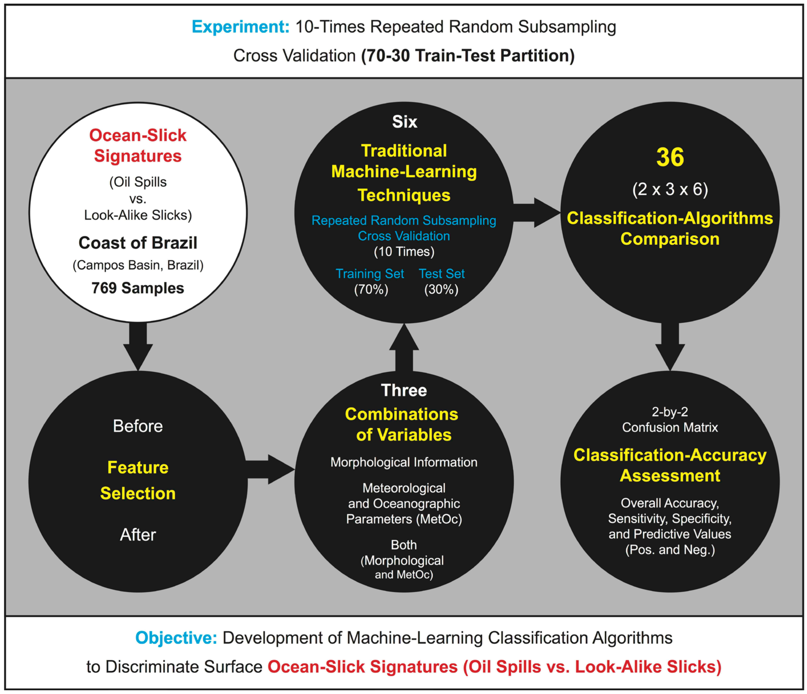
2.1. Research Strategy of Our Training and Testing Experiment

This experiment was divided into five stages as shown by the black circles on the flow diagram in Figure 1. Two ways of feature-set reduction were investigated: (i) typical feature-selection approaches were explored; and (ii) the combinations of variables were divided by attribute-type characteristics (Section 2.1.1 and Section 2.1.2). Traditional ML classification techniques were then applied (Section 2.1.3), leading to the definition of the ML classification algorithms to be tested (Section 2.1.4) and evaluated (Section 2.1.5).

2.1.1. Stage 1: Feature Selection

Feature selection aims, in general, to reduce the dataset size (i.e., dimensionality reduction) at the same time as achieving a more efficient analysis [44]. Feature selection ranks the individual attributes of a given dataset, such that features can be considered useful with respect to the purpose of the study (in our case, classification) based on their relevance and redundancy [45]. Different feature-selection approaches have been proposed in the literature—those most frequently used are reviewed in [39,46,47].
Here, in the search for the most favorable feature subset, seven popular feature-selection approaches were investigated: (i) Information Gain (Info gain [48,49]), (ii) Gain ratio [50,51]; (iii) Gini [52]; (iv) Multifactor Analysis-of-Variance (ANOVA [53]); (v) Chi square (χ² [54]); (vi) ReliefF [55]; and (vii) Fast Correlation Based Filter (FCBF [56]). From this pool of approaches, only one was held to establish the most important variable set to be carried to the next stages. The selected approach was defined by comparing the feature-ranking results of each approach one to another. The following stages of this experiment were performed twice:
-
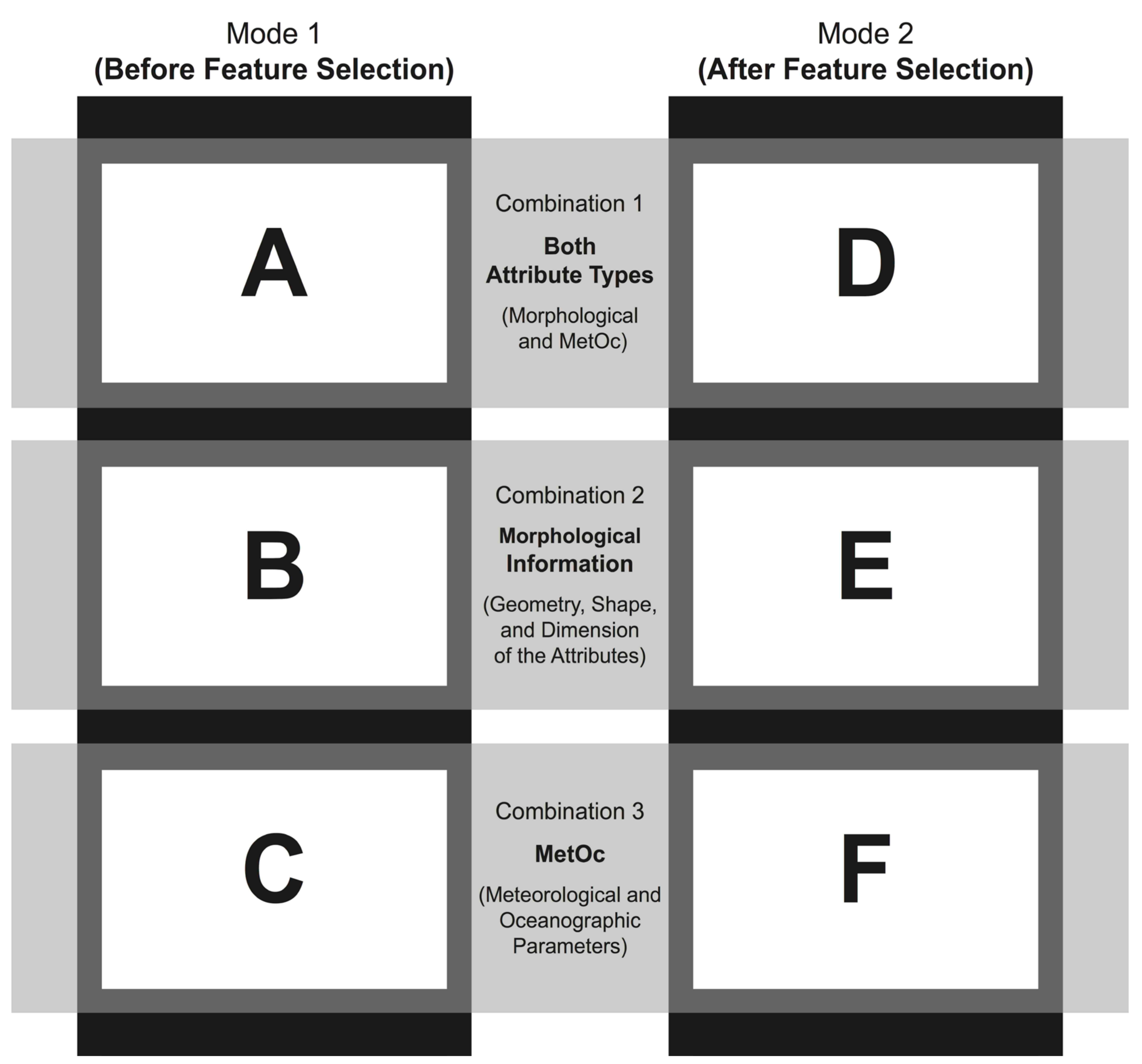
Mode 1: Before feature selection; and
-
Mode 2: After feature selection.

2.1.2. Stage 2: Combinations of Variables

The database used in our experiment has two types of variables characterizing the ocean-slick targets: morphological information and MetOc parameters—Section 2.2 below. From the knowledge gained from past studies (e.g., [31,32]), we chose to analyze each of these variable types together and separately. As such, three combinations of variables were carried to the next stages:
-
Combination 1: Both attribute types together;
-
Combination 2: Only morphological information; and
-
Combination 3: Only MetOc parameters.

2.1.3. Stage 3: Traditional Machine-Learning (ML) Classification Techniques

We used six traditional ML classification techniques:
-
Naive Bayes (NB);
-
K-nearest neighbor (KNN);
-
Decision tree (DT);
-
Random forest (RF);
-
Support vector machine (SVM); and
-
Artificial neural network (ANN).
Reliable classifier accuracy estimates are usually obtained with “cross-validation” procedures [40]. The simplest type of such procedure is the “holdout method”, in which the dataset is divided into two random and independent partitions: one to train and another to test the classifiers [39]. However, as the estimations of the holdout method are pessimistic (i.e., only a single partition of the initial dataset is used to derive the model), another type of cross validation with bias-reduced estimation is suggested: “repeated random subsampling method”, which, in essence, is the holdout method repeated k times [57]. The third type is the “k-fold cross validation”, in which the dataset is partitioned into k subsets of equal size—one-fold at a time, also repeated k times, is held for testing, while the other folds for training, thus, leading to mutually exclusive subsets in which each sample is used only once in the test set. Other than the first type, the other two cross-validation types benefit fully from the existing samples to repeatedly create training and testing sets [39].
We chose to estimate the accuracy of our classifiers with repeated random subsampling cross validation. Different data-fraction recommendations are found in the literature, e.g., 2/3 to train and 1/3 to test ([39]), 70% (or 80%) for training and the remaining 30% (or 20%) for testing ([58]), etc. As any of these partitions are considered valid, here, we simply selected a fixed 70-30 partition. In our Orange Data Mining set up, we tuned the test set to have a balanced number of class samples in relation to the training set. k was set to 10, and during these repetitions the data samples were randomly selected between train-test sets, and the greatest test accuracy of each algorithm was the one to consider [57]. This procedure occurred for each of the six traditional ML classification techniques.

2.1.4. Stage 4: Classification-Algorithms Comparison

The conjunction of the first stage (before and after feature selection) with the second stage (both types together, morphological information, and MetOc parameters) defined what we refer to as a “variable set”. Those depicted in Figure 2, are:
-
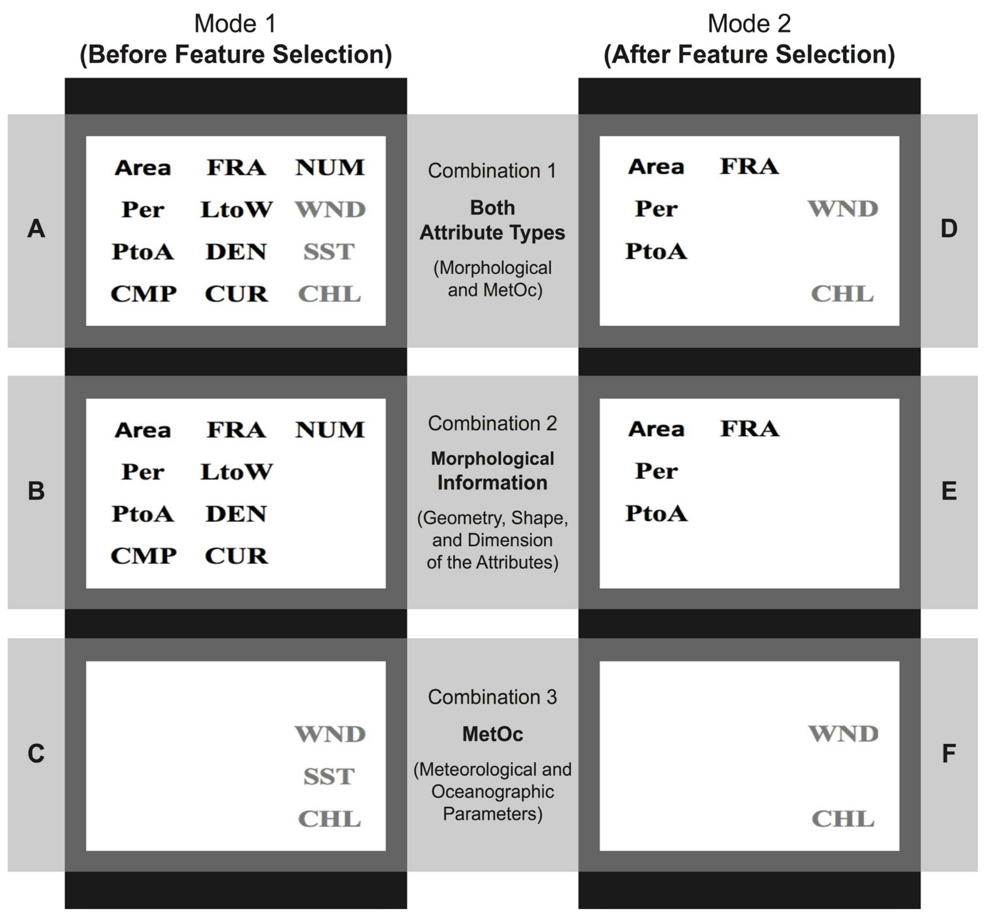
Variable Set A: Mode 1 and Combination 1 (Figure 2A);
-
Variable Set B: Mode 1 and Combination 2 (Figure 2B);
-
Variable Set C: Mode 1 and Combination 3 (Figure 2C);
-
Variable Set D: Mode 2 and Combination 1 (Figure 2D);
-
Variable Set E: Mode 2 and Combination 2 (Figure 2E); and
-
Variable Set F: Mode 2 and Combination 3 (Figure 2F).
The six ML classification techniques applied to these six variable sets resulted in 36 possible outcomes. Effectively, each of these 36 standalone instances formed what we refer to as an “algorithm”. As a result, we have used 36 data-driven ML classification algorithms to address the problem of classifying petroleum signatures observed at the sea surface. As portrayed in Figure 2, the performances of these algorithms were compared in different levels—one should bear in mind the three comparison levels that took place:
-
Primary comparison level: The six techniques were compared among themselves six times using the same set of attributes, i.e., six variable sets (white boxes in Figure 2: A, B, C, D, E, and F);
-
Secondary comparison level: Each technique was compared using different sets of attributes three times before and three times after feature selection (vertical black boxes in Figure 2: A-B-C and D-E-F, respectively); and
-
Tertiary comparison level: Every technique was compared using different sets of attributes two times per combination of variables (horizontal gray boxes in Figure 2: A-D, B-E, and C-F, respectively).
Furthermore, these 36 algorithms were also compared with results from past research [31,32]. These authors also investigated oil spill versus look-alike classification algorithms applied to combinations of similar but different variables than used here; however, they used the simpler LDA technique (Section 2.4.1 below).

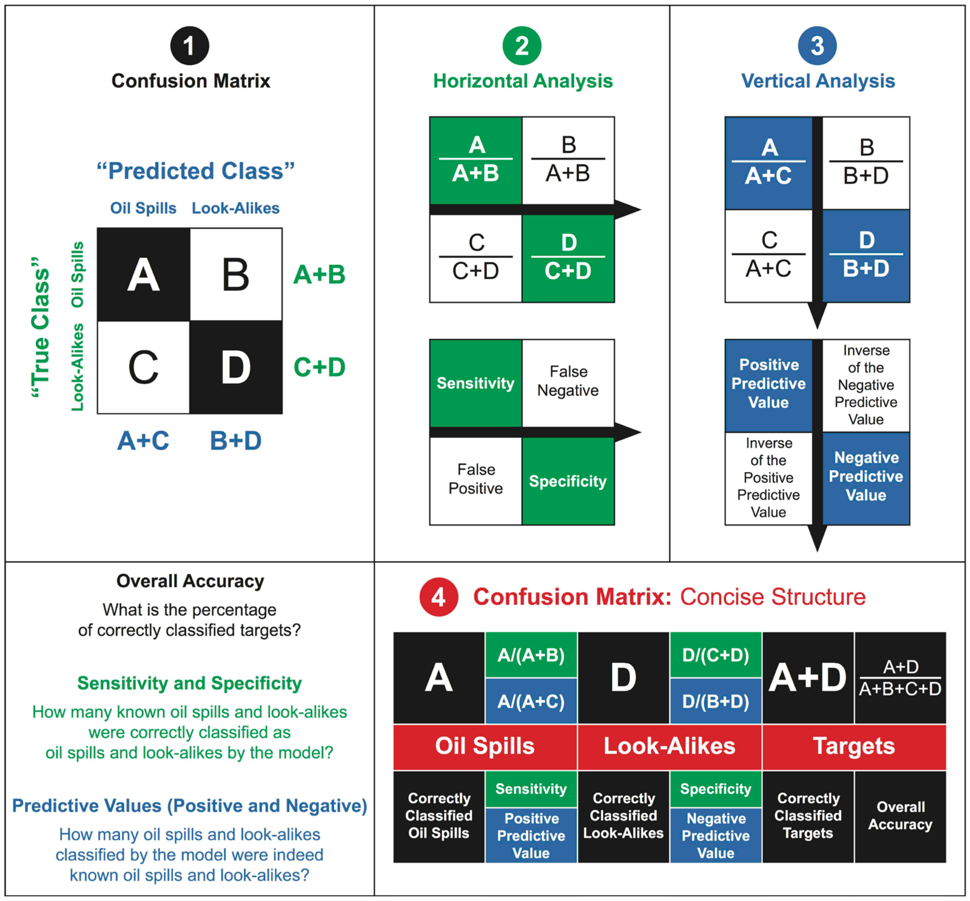
2.1.5. Stage 5: Classification-Accuracy Assessment
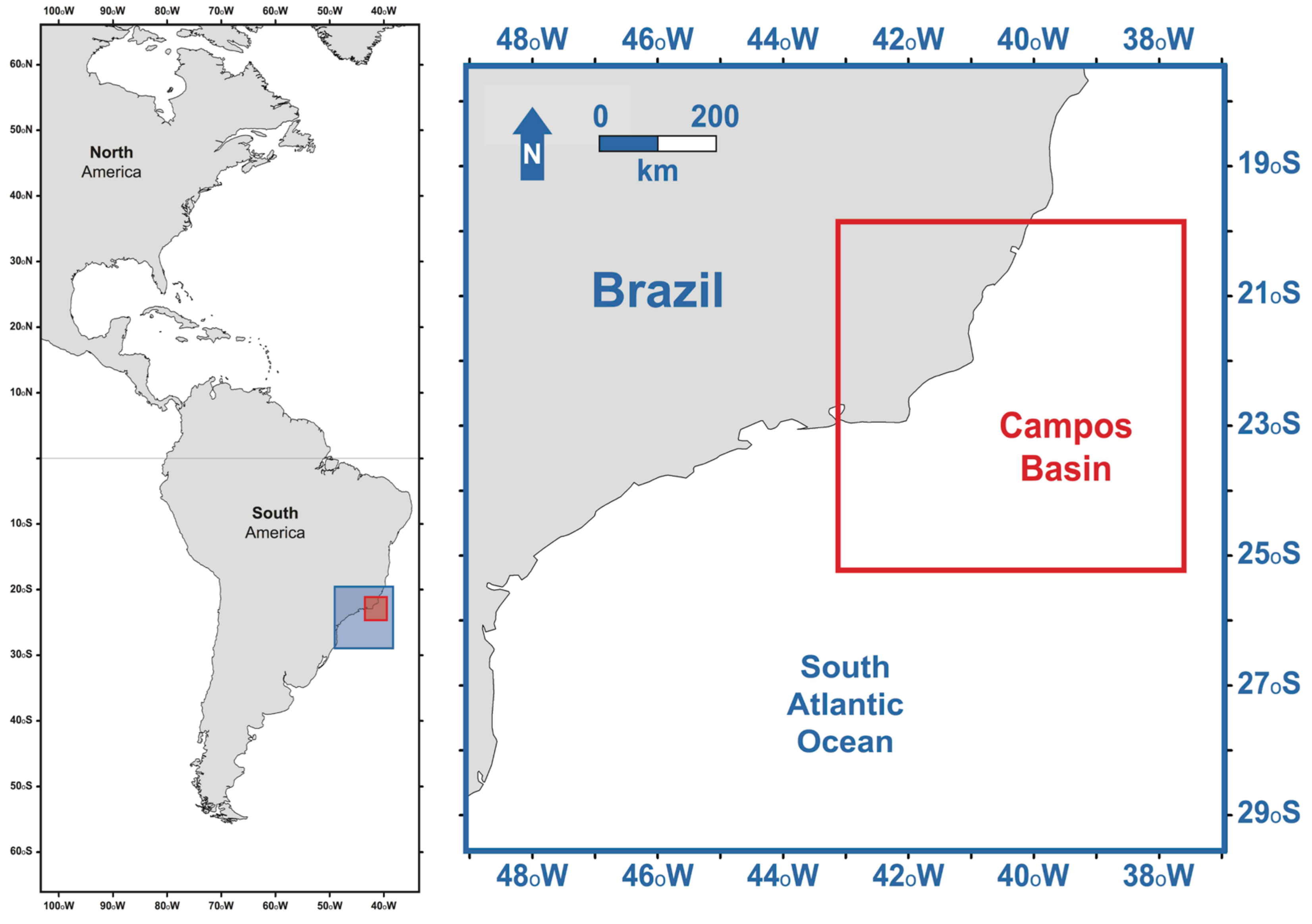
The six ML methods were ranked six times using the same set of attributes, i.e., primary comparison level. This ranking was based on a fundamental performance metric: overall accuracy. Four auxiliary performance metrics were also used to verify the robustness of the algorithms.

2.2. Database

Even though a number of oil slick databases exist and may be obtained in the relevant literature—for instance, from the Gulf of Mexico (e.g., [19,27]) and from the European Seas provided by European Maritime Safety Agency ([59])—the main reason for our database choice is that it has been used in previous studies, also to discriminate spills from look-alikes but with a simpler ML technique (i.e., LDA in Carvalho et al. [31,32]). Those past results are used here as a benchmark to evaluate our findings. Other major assets for this database selection are listed below:
1. It consists of remotely-sensed sea-surface petroleum targets from the Brazilian coast (Section 2.3), being a relevant site to evaluate machine-learning methods to classify oil-slick targets in satellite SAR measurements, and thus discriminating them from look-alike slicks;
2. It is assumed that all observations are independent due to the diverse elements of the satellites, sampling location and time, etc.—relevant environmental aspects of this database are presented in Section 2.3 below; additioanlly, as the spatio-temporal representativeness of the analyzed targets is of great concern, this and other individual characteristics of the database are given in the two subsequent subsections;
3. It comes from validated samples [15];
4. It has a binary classification of each sample as an oil spill or a look-alike slick that was based on human interpretation by specialists and was used here to assess the accuracy of our classifiers (Section 2.4 and Section 2.5);
5. It has a close-to-even class balance between oil spills (n = 350; 45.5%) and look-alikes (n = 419; 54.5%);
6. The 769 samples were taken from 402 RADARSAT-1 scenes from July 2001 to June 2003;
7. Three major types of attributes are present: morphological information, MetOc parameters, and Geo-Loc attributes (the latter one was not accounted for)—see Section 2.2.1 below;
8. Beside the radar satellite data, infrared and visible satellite measurements are included—see Section 2.2.2 below; and
9. It was previously compiled and reviewed by Bentz [15], as well as exploited by Moutinho [60] and Carvalho et al. [31,32].

2.2.1. Train-Test Set (769 Samples)

The 769 instances within the two classes have nine distinct origins. The spill class is associated with oil from four sources: offshore facilities (exploration and production), ship-spills, and confirmed mineral oil from unknown sources (i.e., orphan-spills); no oil seeps were registered. The look-alike class is represented by five environmental events: low-wind speed, upwelling conditions, algal blooms, rain cells, and biogenic films.
The ocean-slick targets in this dataset were described by a number of attribute types, but only two were evaluated here: morphological information and MetOc parameters. Nine pieces of morphological information, describing the geometry, shape, and dimension of the ocean-slick targets, were explored here: area, perimeter (Per), perimeter to area ratio (PtoA), compact index (CMP = (4·Pi·Area)/(Per2)), fractal index (FRA = 2·ln(Per/4)/ln(Area)), length to width ratio (LtoW, i.e., aspect ratio), density (DEN), curvature (CUR), and number of target parts (NUM). Three MetOc parameters, retrieved as averaged values within the limits of the ocean-slicks’ polygons, were explored here: wind speed (WND), sea-surface temperature (SST), and chlorophyll-a concentration (CHL). We did not apply any data transformations, such as log10 or cube root, as in Carvalho et al. [31,32], and thus our evaluations were completed with the non-transformed data.

2.2.2. Satellite Sensors

Our database comprises measurements from the widely used Radarsat-1, which generates C-band HH polarized (transmitting and receiving at horizontal polarization) SAR images with 8-bit digital resolution. These path-oriented images with ground resolutions of 100 m were acquired using two beam modes: ScanSAR Narrow and Extended Low [61].
Measurements from different Earth-Observation System (EOS) sensors provided the MetOc parameters in our database: (i) WND: The SeaWinds scatterometer was a microwave sensor carried by the Quick Scatterometer (QuikSCAT) satellite from 1999 to 2009. It provided sea-surface wind fields with accuracies of <2 m/s and 20° in direction, and nominal spatial resolution of ~25 km [62]; (ii) SST: The Advanced Very High Resolution Radiometer (AVHRR) sensor onboard the National Oceanic and Atmospheric Administration (NOAA) polar-orbiting satellites provided SST measurements with a nominal spatial resolution of ~1 km at nadir [63,64]; and (iii) CHL: Two sensors provided the CHL data: Sea-Viewing Wide Field-of-View Sensor (SeaWiFS) onboard the OrbView-2 satellite ([65]) and Moderate Resolution Imaging Spectroradiometer (MODIS) onboard the Terra satellite ([66]). They both have a nominal spatial resolution of ~1 km at nadir.

2.3. Regions of Interest

The content of the database originates in a specific region of interest off the coast of Brazil: the Campos Basin (Figure 3). This area has vast oil and gas reservoirs, and as in any area with many offshore oil facilities, there have been oil spills from these installations [15]. This basin has dynamic environmental conditions that vary throughout the year and is subject to highly changeable weather, thus guaranteeing good environmental representativeness in our data.
This region is well known for ultra-deep petroleum activities, and its oil and gas platforms are mostly found in deep waters (>1000 m). The main surface-water circulation flow is from northeast to southwest guided by the Brazilian Current, but the region often experiences semi-permanent cyclonic vortices [67]. The meteo-oceanographic conditions in this basin undergo constant easterly winds triggering powerful upwelling lowering the SST to ~11 °C [68]. The upwelled water, originating near Antarctica, not only cools the Campos Basin SST’s, but also brings nutrients to surface layers increasing the primary productivity and CHL detectable from satellites [69].

2.4. Machine-Learning (ML) Methods

As opposed to “deep-learning” methods, the six ML techniques in our analysis have been considered “traditional” ML classification techniques [23]. The six traditional techniques are regarded here as “simple” (NB, KNN, and DT) and “advanced” (RF, SVM, and ANN). Others have proposed different divisions for various ML methods: linear versus non-linear, tree-based versus non-tree-based, etc. [70].
Due to the simplicity of the traditional techniques, compared to deep learning, they are suitable for the objectives of our investigation (i.e., knowledge discovery [39]). Few parameter settings are involved, and, besides, these techniques provide more easy-to-understand, intuitive information leading to improved knowledge from their outcomes [71].
In our practical ML implementations, instead of using the Orange Data Mining default settings, we adopted our own customized setting based on verification among possible optional adjustments. Hyper-parameters are not related to the input data but can affect the final experimental results. NB and DT were the only two methods without any changes in their different hyper-parameter quantities. In KNN, the weight was set to distance. RF underwent two modifications: one in the basic properties (we chose to replicate training) and another in the growth control (subsets were not split). The optimization parameter of SVM did not have an iteration limit. There were three ANN changes: activation (tanh), solver (L-BFGS-B), and with replicate training.
LDA is another simple traditional technique. Although not directly exploited here, LDAs were applied to classify spills and look-alikes reported in past studies [31,32]. The overall accuracy of the LDA classification is used here as a standard benchmark for considering an acceptable performance for the ML classification algorithms, see below. Our selection of traditional ML methods is presented briefly below, from basic to more sophisticated, with references provided for more detailed information.

2.4.1. Performance Benchmark

-
Linear Discriminant Analysis (LDA): This is one of the simplest, long-established techniques widely used for classification problems [40,72]. LDAs focus on maximizing the separability between the known classes by computing a set of discriminant functions and thus allocating a sample to the class of maximum function value. Although several LDA extensions and variations exist (e.g., flexible, global-local, quadratic, dual-space, null-space, regularized, penalized, probabilistic, etc.), the considered one is the regular LDA derived from the Fisher LDA—in which only linear combinations of inputs are used [26].
-
Past LDA Papers: Carvalho et al. [31,32] published LDA analyses to classify spills from look-alikes. Even though these past studies used the same dataset used here (Section 2.2), they did not carry out cross validation and all samples were used in their training phase. While Carvalho et al. [31] used all 769 samples, Carvalho et al. [32] performed quality-control filters and only used 560 samples. They exploited various combinations of variables using morphological information and MetOc parameters: Carvalho et al. [31,32] compared 39 and 114 combinations of variables, respectively; these included the application of different data transformations (i.e., log10 and cube root). Their best non-transformed overall-accuracy LDA results, using the same combinations of variables to those defined here in Section 2.1.2 (i.e., both types together, only morphological information, and only MetOc parameters), are taken as our benchmark. These are shown in Table 1: ~83% with morphological and MetOc attributes, ~79% only morphological information, ~77% only MetOc parameters. When other combinations, using aspects of morphological and MetOc attributes, were used, a slightly improved overall accuracy of ~84% was reached ([31]), and further progress was possible when a Geo-Loc attribute (bathymetry) was accounted for: ~85% ([32]). The other four performance metrics ranged between ~73% and ~91% (Table 1).

2.4.2. Simple Techniques

-
Naive Bayes (NB): This simple technique is derived from the application of Bayes’ theorem of posterior probability—it is often named as naive Bayes (NB). Bayesian classifiers often outperform, or are comparable in performance to, more powerful classifiers and are faster in terms of computer time [73]. The class membership probabilities are predicted by a given sample belonging to a specific class. In this technique, it is assumed that the influence of the values of the variables on any class does not affect the values of the other variables—this is known as class conditional independence [39]. Indeed, because of the assumption that the variables are independent of the classes, the application of the Bayes’ theorem is considered “naive” [39].
-
K-Nearest Neighbor (KNN): This method works as follows: in the attributes n-dimensional space, it seeks the k closest samples among all existing samples, i.e., each time it predicts a new sample, it searches the “nearest neighbor” in the entire dataset used for training [40,74]. The value of k, the number of neighbors, used here was 5. The measure of closeness is given by a metric distance, e.g., Euclidean distance. Different from all other methods analyzed here, KNN is regarded a “lazy learner”, mostly because it creates numerous local target function approximations making them slower and only able to generalize once needed, as opposed to the other five techniques that are “eager learners”, as they create a global approximation and can generalize before a query is given [39].
-
Decision Tree (DT): Decision trees are tree-structure flowcharts. In this top-down recursive tree-induction method, the internal nodes (i.e., non-leaf nodes) indicate tests per attribute and the tree branches correspond to the test outcomes. Terminal nodes (i.e., leaf nodes) represent the predicted class label, while the uppermost node is known as the root node [39].

2.4.3. Advanced Techniques

-
Random Forest (RF): This technique is one of the many types of ensemble methods, i.e., it combines the learning from a series of other individual methods [75]. RFs can be considered as a collection of DTs, which gives rise to the name “forest”, with a flowchart-like tree structure [76,77]. In simple terms, each of these DTs start with a “random” choice of variable, and the chosen class of each sample is given by the vote of each DT.
-
Support Vector Machine (SVM): This technique can classify any sort of data, i.e., both linear and nonlinear, with a smaller chance of suffering from overfitting than other methods [39]. This non-tree-based classifier transforms the original data into a higher dimension level to search for a unique and optimal hyperplane, i.e., a linear decision boundary [78]. This hyperplane separates the classes in this new multidimensional feature space, and, in general terms, this separates the data by using selected essential training samples—the so-called “support vectors” [79]. From these vectors, the maximal margin between the two classes is defined [80,81]. There is a compromise between reaching high accuracies and long processing times [82]. Other reference sources are: Cherkassky and Ma [83], for the selection of hyper-parameter settings, and Mountrakis et al. [84], for broad review of remote-sensing data SVM applications.
-
Artificial Neural Network (ANN): ANNs, commonly referred to as “neural networks”, try to mimic the way human “neurons” connect to each other [39]. This neuron-like process consists of several node layers made of two units: input unit (input layer) and output unit (this output layer may contains one or more in-between hidden layers—neurodes) [85]. A multilayer ANN with a single hidden layer is said to be a two-layer network—the input layer is not counted because it only delivers the input information [39]. The network nodes, also known as “artificial neurons”, have an organized, developed structure and are fully interconnected—when one node feeds the next node, weights and thresholds are associated with the passing of information at each connection [39]. While the input corresponds to the values of the attributes used in the training samples, the output is the prediction for those samples [39]. The ANN learns from these connections while it adjusts the weights, so it is able to predict the class label of each sample. This ANN learning process is known as connectionist learning [39]. Even though ANNs are capable of handling noisy data, they usually have long run times, have a long list of required hyper-parameter settings, and are difficult to interpret, as compared to other advanced techniques, e.g., SVM [71].

2.5. Algorithms’ Accuracies

We use the standard approach of classifying sea-surface targets by comparing the “predicted class” (i.e., independent case) with those from the “true class” (i.e., dependent case) [39]. The former class accounts for the classification model outcome and the latter class is represented by categorical memberships determined by specialists.
Here, our accuracy assessments were evaluated based on information extracted from 2-by-2 confusion matrices (Figure 4: Panel 1)—five performance metrics were exploited: a fundamental one (i.e., overall accuracy) and four auxiliary ones (i.e., sensitivity and specificity, and positive and negative predictive values) [86]. Panels 2 and 3 of Figure 4 demonstrate how the auxiliary performance metrics are calculated. Other terms are found in the literature referring to sensitivity (e.g., “recall”) and positive-predictive value (e.g., “precision”) [87]. In addition, sensitivity and specificity are frequently referred to as “producer’s accuracy”, whereas the predictive values are termed as “user’s accuracy” [88].
Even though we express our results as ranks based on the fundamental overall-accuracy metric, the other four auxiliary performance metrics are also important in determining the overall success of the classifiers, as these metrics corroborate the individual achievements of the algorithms by verifying the misclassification tradeoff [89]. An effectiveness limit was set to evaluate the algorithms’ accuracies: 60% [27,28,29,31,32]. If any of these metrics fall below this level, the algorithms are considered ineffective, referred to as being null and void. Figure 4 (Panel 4) outlines the structure accounting for all five accuracy-assessment metrics in a single table.
Other ways are found in the literature to assess the performance of classification algorithms, including the area under the curve (AUC) [90]. The combination of two auxiliary performance metrics provides another possible performance metric: the F-measure, i.e., the square root of sensitivity times the positive-predictive value [91]. These two performance metrics are better for problems with imbalanced classes ([39]), which is not the case here.

3. Results

3.1. Feature Selection (Stage 1)

Feature-selection ranks were found not to be the same for the seven feature-selection approaches. Discrepancies occurred among the different selection approaches, i.e., the importance given to each attribute varied. Three approaches produced similar rankings (Info gain, Gain ratio, and Gini), whereas the other four approaches (ANOVA, χ², ReliefF, and FCBF) presented quite different rankings. After comparing the results from these seven approaches, and analyzing the similarities and divergence of all rankings, the decision was made to use those from Info gain, given in Table 2.
The decision limit (or stopping criteria) to select variables based on the values of feature-selection ranks is user defined [39]. Therefore, the “best” attributes were separated by the “worst” ones by a specific cutoff threshold that we determined from the ranking values. Taking the most important variable as a reference, the relative importance of the other variables was computed—for example, the highest ranked variable was PtoA (its rank was 0.224), whereas the second and third ranked variables were Area (0.215) and WND (0.191); so, their relative-importance percentages in relation to PtoA were 95.8% and 85.4%, respectively, as shown in Table 2.
After evaluating the Info gain rank values and their relative percentage of importance, a calculated cutoff threshold was set to 35% relative to the highest variable’s rank. As a result, variables with ranks below 0.078 were discarded—i.e., six variables were considered “less discriminative” and eliminated: NUM, DEN, SST, CUR, LtoW, and CMP. This reduced the attribute-wise dataset size by half (Table 2). The six “most representative” attributes ordered by the Info gain ranking are: PtoA, Area, Per, and FRA (four morphological pieces) and WND and CHL (two MetOc pieces). These are indicated in Table 2 with an asterisk. Note that: (i) before feature selection (Mode 1), the ML algorithms used all twelve attributes in our database (vertical black box on the left side of Figure 2: A, B, and C); and (ii) after feature selection (Mode 2), the ML algorithms only used the attributes selected with Info gain (vertical black box on the right side of Figure 2: D, E, and F).
Additionally, when only the six pieces of morphological information, or three MetOc parameters, were used separately in any of the feature-selection approaches, the ranking values for each variable did not change. This is because feature-selection evaluates the importance of each variable, so the ranking should not alter if variables are removed or included [39]. On the other hand, the removal or inclusion of samples (not performed here) may alter the individual variable importance.

3.2. Combinations of Variables (Stage 2)

Feature selection identified the attributes within the six “variable sets” defined by the two feature-selection modes and the three combinations of variables: A) All twelve variables; B) The nine pieces of morphological information; C) The three MetOc parameters; D) All selected attributes; E) Only the four selected morphological information; and F) Only the two MetOc parameters. Figure 5 illustrates these six variable sets that were applied to the six ML methods forming the 36 algorithms evaluated in the primary comparison level (white boxes in Figure 2). Variable sets A, B, and C represent those from before feature selection (Mode 1), whereas variable sets D, E, and F are those from after feature selection (Mode 2)—these two groups of variable sets were used in the secondary comparison level (vertical black boxes in Figure 2 and Figure 5). Another grouping accounted for pairs of variable sets corresponding to each of the defined combinations of variables: A and D (Combination 1: both attribute types together), B and E (Combination 2: only morphological information), and C and F (Combination 3: only MetOc parameters)—these three groups of variable sets were used in the tertiary comparison level (horizontal gray boxes in Figure 2 and Figure 5).

3.3. Classification-Accuracy Assessment (Stage 5)

The performance and effectiveness of the six traditional ML classification techniques were evaluated alongside the classification-accuracy assessment of the 36 data-driven ML classification algorithms (Figure 6 and Figure 7). This section presents the performance findings reported in both figures: Figure 6 contains six tables visually aligned with the comparison levels portrayed in Figure 2 and Figure 5, whereas Figure 7 graphically represents some of the tabular outcomes in Figure 6.
The six tables in Figure 6 correspond to the variable sets (Section 2.1.4 and Section 3.2) and have the ML methods ordered from what we previously considered basic to more sophisticated—simple (NB, KNN, and DT) and advanced (RF, SVM, and ANN). This ordering is used to aid the visual comparison of the algorithm performance. Each table in Figure 6 has the six ML methods ranked by the cross-validation test-set overall accuracy. These methods have also been colored to facilitate several comparisons: green (most effective algorithm), blue (second and third most successful), orange (fourth and fifth ranks), and red (least accurate algorithm)—as given by the primary comparison. The best and worst of all 36 algorithms are indicated (++ and −−), as are the best and worst for each feature-selection mode (+ and −). The comparisons below are presented in subsections per comparison level: primary, secondary, and tertiary.
The evaluations in the primary comparison level used the same sets of variables for the six ML methods (white boxes in Figure 2, Figure 5, and Figure 6). At the other two comparison levels, each algorithm was compared using different sets of attributes. However, different sets of attributes in the secondary level refer to exploiting different attribute types (vertical black boxes in Figure 2, Figure 5, and Figure 6), whereas the tertiary level relates to having variables of the same type (horizontal gray boxes in Figure 2, Figure 5, and Figure 6). In the latter level, the exception is in Combination 1 that uses both attribute types.
The two panels shown in Figure 7 illustrate the overall-accuracy information shown in Figure 6—while panel 1 (left) focuses on the six traditional ML classification techniques as in the primary comparison level, panel 2 (right) depicts the feature-selection modes from the secondary comparison level.

3.3.1. Primary Comparison Level

This section refers to the six white boxes in Figure 2, Figure 5, and Figure 6.
-
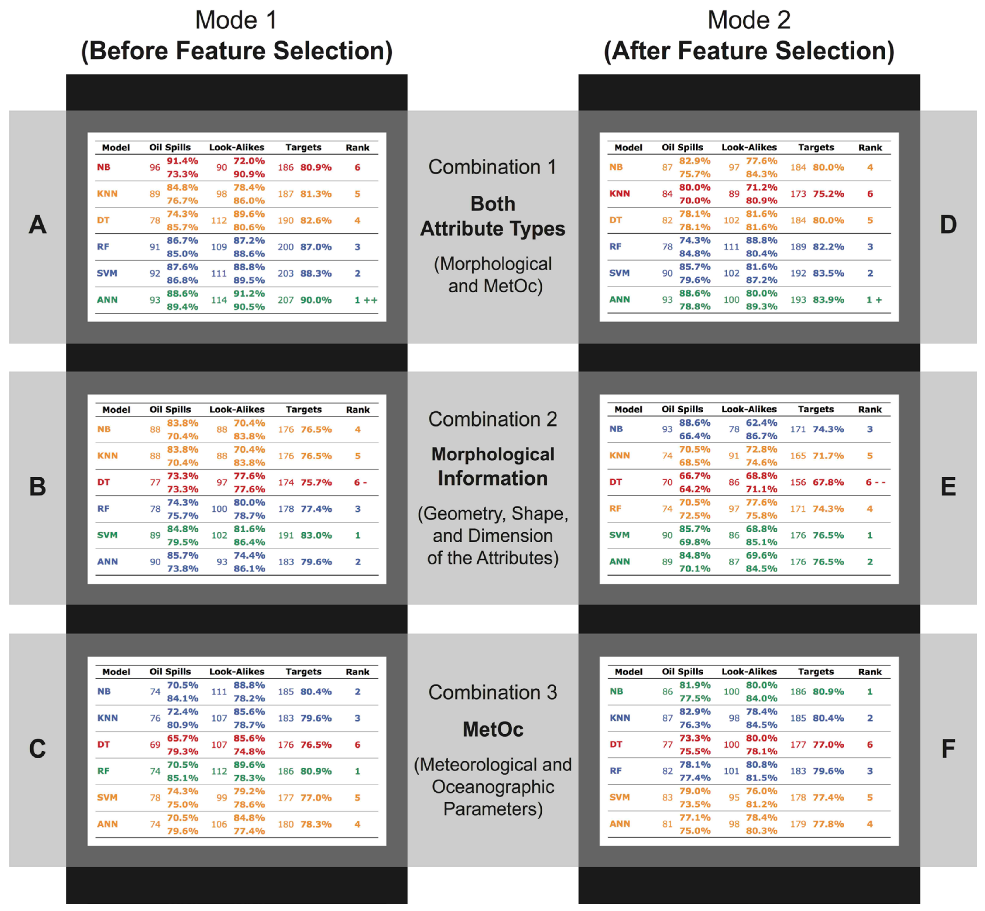
Variable Set A: Figure 6A shows the results of using all twelve variables without feature selection: Area, Per, PtoA, CMP, FRA, LtoW, DEN, CUR, NUM, WND, SST, and CHL (Figure 5A: variable set A). ANN achieved the best accuracy (90%), which was also the most accurate of all 36 algorithms (shown by ++). Such accuracy outperformed the least accurate algorithm in this level by 9.1 percentage points: NB (80.9%). This was the largest overall-accuracy difference between the best and worst accuracy per variable set (Figure 7).
-
Variable Set B: Figure 6B shows the results of using the nine pieces of morphological information prior to feature selection: Area, Per, PtoA, CMP, FRA, LtoW, DEN, CUR, and NUM (Figure 5B: variable set B). SVM was the most accurate algorithm (83%) outperforming the least accurate one by 7.4 percentage points: DT (75.7%).
-
Variable Set C: Figure 6C shows the results of using the three MetOc parameters before feature selection: WND, SST, and CHL (Figure 5C: variable set C). RF reached the highest accuracy (~81%) with 4.3 percentage points from the least accurate: DT (76.5%). This overall-accuracy difference was one of the smallest of all variable sets (Figure 7).
-
Variable Set D: Figure 6D illustrates the outcomes of using the six feature-selected attributes from both attribute types: PtoA, Area, WND, Per, FRA, and CHL (Figure 5D: variable set D). As in Figure 6A, ANN was the most accurate algorithm (~84%). This top accuracy is not just for this specific variable set, but was also the highest accuracy among all variable sets that used feature-selected variables (Figure 7). As shown, feature selection reduced the accuracy by ~6 percentage points.
-
Variable Set E: Figure 6E shows the outcomes of using the four feature-selected morphological information: PtoA, Area, Per, and FRA (Figure 5E: variable set E). SVM and ANN tied as the most successful algorithms at ~76% but this was the lowest of all best accuracies within all six variable sets. The least accurate algorithm was DT (~68%), which was also the least accurate of all 36 algorithms (indicated by −−).
-
Variable Set F: Figure 6F illustrates the outcomes of using the two feature-selected MetOc parameters: WND and CHL (Figure 5F: variable set F). This was the only case in which a simple technique outperformed the advanced ones: NB reached the highest accuracy (~81%) at 3.9 percentage points above the least-accurate simple technique: DT (77%). This was the smallest overall-accuracy difference between the best and worst classifiers (Figure 7).
Table 3 reviews the best and worst results per variable set.

3.3.2. Secondary Comparison Level

Here we discuss the contents of the two vertical black boxes in Figure 2, Figure 5, and Figure 6.
-
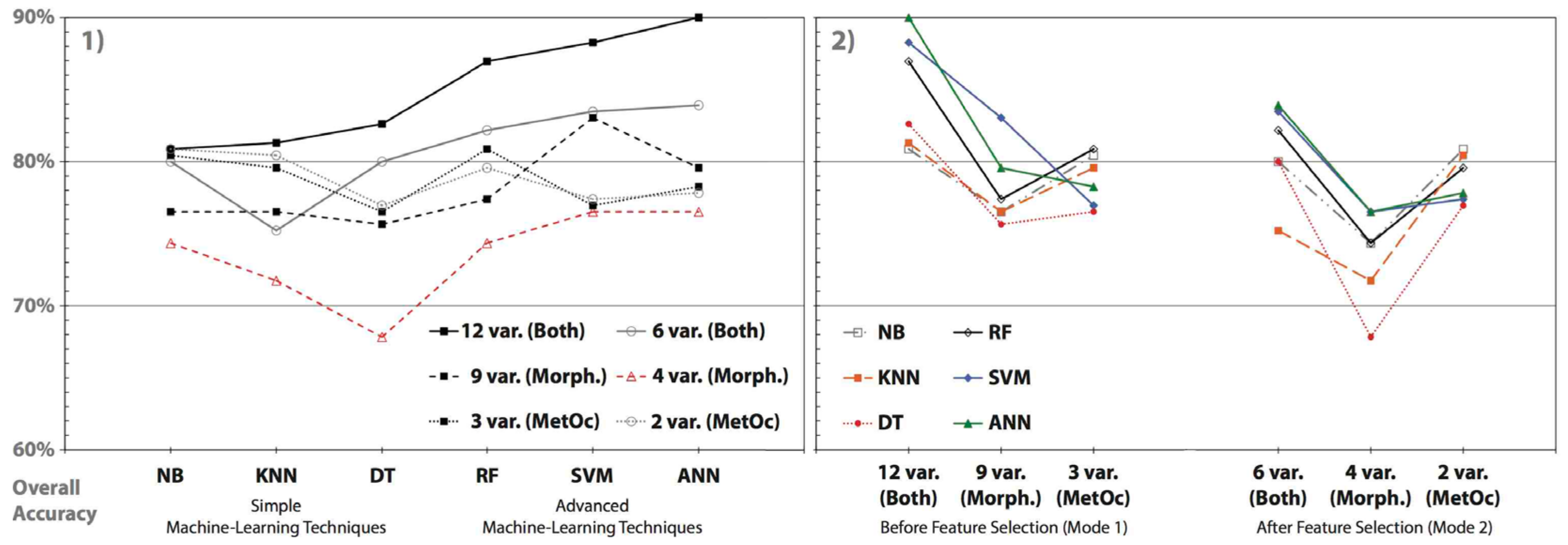
Mode 1 (Before Feature Selection): Most techniques (NB, KNN, DT, and RF) were more accurate when all variables of both attribute types were used (Combination 1) and performed worse with morphological information (Combination 2); Figure 7. However, two advanced techniques (SVM and ANN) were best when using all variables of both attribute types (Combination 1), but were less accurate with MetOc parameters (Combination 3).
-
Mode 2 (After Feature Selection): The pattern observed above was also frequent in most techniques (DT, RF, SVM, and ANN); Figure 7. These were also more accurate when exploiting variables from both types (Combination 1) and were also less accurate when accounting for morphological information (Combination 2). Here, two simple techniques (NB and KNN) deviated from this pattern and were more accurate with MetOc parameters (Combination 3) and less accurate with morphological information (Combination 2).
Table 4 presents the best and worst results per ML method.

3.3.3. Tertiary Comparison Level

This section concerns the three horizontal gray boxes in Figure 2, Figure 5, and Figure 6.
-
Combination 1 (Both Attribute Types): the six techniques were more accurate before (A) than after (D) feature selection. The variable set A provided the best of all 36 algorithms: ANN (90%)—indicated in Figure 6A by ++. The overall-accuracy difference between the best and worst algorithms within A, and well as D, was about ~9%.
-
Combination 2 (Morphological Information): without exception all six algorithms performed better before (B) than after (E) feature selection. The variable set E provided the worst performance of all 36 algorithms: DT (~68%) indicated by −− in Figure 6E. As in Combination 1, the overall-accuracy difference between the best and worst algorithms within B, and well as E, were also about ~9%.
-
Combination 3 (MetOc Parameters): Only RF and ANN better performed before feature selection (C) than after (F), as this pattern was inverted for the other ML methods that reached improved outcomes with fewer variables (after feature selection: F) than with more variables (before feature selection: C). In both variable sets (C and F), the algorithms produced the smallest overall-accuracy differences between the best and worst algorithms of all (~4%); about half of those from the other four variable sets, i.e., A, B, D, and E.

3.4. LDA Benchmark Comparison

Our overall-accuracy benchmark is presented in Table 1. Those LDA accuracies were reached with the same database used here and included all variables of both types together and separately [31,32]. Hence, we focus on comparing them to our 18 algorithms that used variable sets before feature selection for a fair comparison (Figure 2, Figure 5, Figure 6 and Figure 7):
-
LDA 1 (83.1%): This is analogous to those using variable set A (Mode 1 and Combination 1), and was outperformed by all advanced techniques (RF (87.0%), SVM (88.3%), and ANN (90.0%)) but was more effective than all simple ones (NB (80.9%), KNN (81.3%), and DT (82.6%)).
-
LDA 2 (79.1%): This used variable set B (Mode 1 and Combination 2) and was only inferior to SVM (83.0%) and ANN (79.6%); but other algorithms were less accurate.
-
LDA 3 (76.9%): This algorithm matched variable set C (Mode 1 and Combination 3) but performed worse than all algorithms except DT (76.5%).
-
LDA 4 (83.7%): This was the best of all 39 combinations reported by Carvalho et al. [31], also using variables from both attribute types, and performed better than 34 of our algorithms, besides the ones that were better than LDA 1 and ANN with both attribute types after feature selection (83.9%).
-
LDA 5 (84.6%): Carvalho et al. [32] were able to improve the LDA accuracy by combining the two attribute types with a Geo-Loc attribute (bathymetry). They explored 114 different combinations of variables.

4. Discussion

The bipartite train-test set of the repeated random subsampling cross validation method (70-30 partition), accompanied by balanced sample-class sets and test-phase accuracy estimations, secured unbiased classification outcomes. Additionally, our classifiers undergoing 10-times repeated random subsampling cross validation produced a good capability for generalization [41].
One of the few other studies that compared various ML methods to classify ocean-slick signatures in satellite imagery was by Xu et al. [36]. As a feature-selection approach they used permutation-based variable accuracy importance [92]. They adopted different criteria to produce a different set of selected variables to each ML method they analyzed. This formed a comparison of different techniques that used different variables, as opposed to here, where we compared different techniques using the same set of attributes—i.e., primary comparison level: white boxes in Figure 2. However, in the other two comparison levels considered here, there were comparisons of the same technique using different sets of variables—i.e., secondary and tertiary levels: vertical black boxes and horizontal gray boxes in Figure 2, respectively.
One could argue that our database should contain more data to demonstrate the reliability of the conclusions of our paper due to the number of instances analyzed here: 769 samples. Indeed, it is a smaller quantity than those of other studies found in the literature (e.g., ~5000 in Carvalho [19] or Carvalho et al. [27,28,29]) but was, however, a larger quantity when compared to other published studies (e.g., Xu et al. [36], Mattson et al. [93], and Cao et al. [94], that only used 198, 194, and 267 samples, respectively). In fact, we are using the same dataset as in past studies, i.e., [31,32]. It is believed that the more data available, the better the result might be, but the number of samples in a database should not always be the only consideration as data quality is also important. Regarding the matter of data quality: (i) our database comes from a relevant site in the Brazilian coast (Campos Basin) where oil spills and look-alike slick targets are observed; (ii) the diverse elements of our database (i.e., satellites, sampling location and time, among others) undertake the sampling observations as independent; (iii) the samples have been validated [15]; (iv) there is a close-to-even split class balance (spills (n = 350; 45.5%) and look-alikes (n = 419; 54.5%)); (v) the 769 samples came from 402 different RADARSAT-1 scenes spanning two years (July 2001 to June 2003); (vi) two types of attributes have been concomitantly explored (morphological information and MetOc parameters); (vii) radar, infrared and visible satellite measurements are accounted for.
The results presented in Section 3.3, regarding classification-accuracy assessment, arose from our empirical observation; we do not intend to state new ML theorems. Our findings may be data-specific, as our comparison occurred using a specific dataset with various sets of attributes of different attribute types.
The comparisons at the primary level (Section 3.3.1) demonstrated that the advanced techniques (RF, SVM, and ANN) reached superior accuracies than the simpler ones (NB, KNN, and DT); Figure 7. The one exception (variable set F accounting only for two MetOc parameters, Figure 6F) was where NB was best. The highest accuracies were usually those from ANN and SVM, with three and two of the most effective outcomes. The algorithms with the poorest performance were from simple techniques, in which DT accounted for four of the six lowest scores. All algorithms performed well, from ~62% and >90% (overall accuracy). As such, considering our 60% limit to accept an algorithm as effective, none of the 36 algorithms were deemed null and void. Of the 144 possible values for the auxiliary metrics, only ten were below 70%; nine of which were in the variable set E: after feature selection (Mode 2) and only morphological information (Combination 2)—Figure 5E and Figure 6E. When using this variable set, only RF had all five performance metrics above 70% (Figure 6E).
The comparisons at the secondary level (Section 3.3.2) demonstrated that most techniques were superior when using variables from both attribute types (morphological and MetOc) and less accurate when using morphological information alone (Figure 7). This pattern of better performance with Combination 1 occurred ten of the possible twelve times, with Combination 3 giving best accuracies for the other two (Table 4). One could argue that having more variables, as in Combination 1, which accounts for both attribute types, would include more information, thus ensuring better accuracies. However, our results reveal that it is not the quantity of variables that matters the most, as morphological information (9 and 4 variables) accounted for more variables than MetOc parameters (3 and 2 variables). The main factor controlling the accuracy of the algorithms is the variable type: morphological versus MetOc. The pattern of having the worst performance with Combination 2 occurred ten of the possible twelve times, with Combination 3 giving worst accuracies for the other two (Table 4). Better accuracy results with only morphological information, than with only MetOc parameters, was not found by Carvalho et al. [31,32] in their LDA analyses, in which they observed the opposite (Section 3.4).
The simple techniques (NB, KNN, and DT) were usually more accurate than the advanced ones (RF, SVM, and ANN) when less complexity was involved (i.e., fewer variables were included—MetOc parameters only) than when more attributes were included (Figure 7). The opposite held true for the more advanced techniques, which dealt well with more variables (i.e., reached higher accuracies—both attribute types) than in the cases with fewer variables. This is apparent in the color-coding of Figure 6: while A and D account for more variables, the advanced techniques are green and blue (1st, 2nd, and 3rd ranks) and the simple ones are orange and red (4th, 5th, and 6th ranks). This pattern is inverted in C and F that account for fewer variables: simple (green and blue) and advanced (orange and red). In the center variable sets (morphological information: B and E) there was a transition from more to fewer variables; for B (more variables: 9 without feature selection) the advanced techniques were superior and in E (fewer variables: 4 with feature selection) the simple techniques performed slightly better (Section 3.3.3). These patterns may be related to quantity (more versus fewer variables), quality of the variables (attributes type: both versus only MetOc parameters), and complexity of the technique.
In general, most comparisons at the tertiary level (Section 3.3.3) revealed a pattern in which the better-performing algorithms used more variables (before feature selection: A, B, and C) while lower accuracies resulted from using fewer variables (after feature selection: D, E, and F); this was independent of the Combination considered (Figure 6 andFigure 7). In Combination 3, NB, KNN, DT, and SVM were exceptions. Such a pattern occurred in different sets of variables of the same attribute type; even though Combination 1 accounts for both attribute types, it also yields better accuracies with more (A) than with fewer (D) variables. Likewise, Table 3 andTable 4 indicate that the algorithm accuracies tended to decrease after the feature-selection attribute removal. This may indicate that important variables have been eliminated by feature selection. Perhaps the cutoff threshold of 35%, used to reject variables based on the ranking results, could be relaxed (Table 2).
The overall-accuracy difference between the best and worst algorithms of Combinations 1 or 2 showed greater variations between the best and worst performances (~9%). The use of Combination 3 had half of that difference (~4%). These overall-accuracy differences were independent of the variable set. This difference may indicate that using more attributes, i.e., Combination 1 (12 and 6 variables) and Combination 2 (9 and 4 variables), brings more complexity to the classification than using fewer attributes, i.e., Combination 3 (3 and 2 variables). Such complexity would lead to the advanced techniques outperforming the simple ones. Perhaps it indicates that since there are errors and uncertainties in all measurements, these overwhelm the information the additional attributes bring to the problem. This indicates a study is needed to determine the adjustments, if any, of the ranking caused by inherent inaccuracies in the measurements.
The LDA benchmark comparison (Section 3.4) showed that both papers, i.e., [31,32], reported a clear stratification on overall-accuracy ranking of the algorithms: those using both attribute types were better than those using morphological information, followed by MetOc parameters. However, we did not observe this pattern. On the contrary, MetOc outperformed morphological; here, each were less effective than using both types together. One possible explanation for this disparity could be the number of combinations of variables explored in each study: while Carvalho et al. [31,32] compared 39 and 114 combinations of variables, respectively, we only compared six combinations; three before and three after feature selection. More research is needed to explain the differences in these results.

5. Summary and Conclusions

This study fills a scientific gap by comparing and evaluating six traditional machine-learning (ML) classification techniques applied to several combinations of satellite-retrieved attributes to classify petroleum targets observed at the sea surface (Campos Basin, Brazil; Figure 3). We implemented a series of 36 ML classification algorithms that were evaluated with 10-times repeated random subsampling cross validation. These algorithms produced a good capability of generalization, as defined by their test-set overall accuracy estimations, achieved with 70-30 train-test partition and balanced class sets (Figure 1). 769 ocean-slick signatures, imaged in 402 RADARSAT-1 scenes (2001–2003), were analyzed here: oil spills (350; 45.5%) and look-alike slicks (419; 54.5%).
Simple techniques (naive Bayes (NB), K-nearest neighbor (KNN), and decision trees (DT)) were compared with advanced techniques (random forest (RF), support vector machine (SVM), and artificial neural network (ANN)). Our data analysis experiment exploited two types of attributes: morphological information (area, perimeter (Per), perimeter to area ratio (PtoA), compact index (CMP), fractal index (FRA), length to width ratio (LtoW), density (DEN), curvature (CUR), and number of target parts (NUM)) and Meteorological and Oceanographic (MetOc) parameters (wind speed (WND), sea-surface temperature (SST), and chlorophyll-a concentration (CHL)). Five performance metrics were used to evaluate our results: sensitivity, specificity, positive- and negative-predictive values, and overall accuracy (Figure 4). Feature selection was accomplished (Information gain) and, based on the importance given to each attribute, the dataset size was reduced by half (PtoA, Area, Per, FRA, WND, and CHL) with a stopping criterion set to a relative importance of 35% of the highest variable’s rank (Table 2). The ML based comparison occurred at different levels:
-
Primary: techniques compared among themselves;
-
Secondary: techniques compared using different types of attributes: before (Mode 1) and after (Mode 2) feature selection; and
-
Tertiary: techniques compared using different types of attributes: both types together (Combination 1), morphological information (Combination 2), and MetOc parameters (Combination 3).
The conjunction of the two Modes with the three Combinations defined the six variable sets. The most important results are listed below (Figure 2, Figure 5, Figure 6 and Figure 7).

5.1. Primary Comparison Level

Advanced techniques were usually superior to the simpler ones (Table 4). Of the six variable sets, ANN and SVM had three and two best performances, whereas the poorest performance was from DT with four lowest scores (Table 3).
Considering the fundamental performance metric (overall accuracy), an algorithm using ANN was the most effective of all 36 (90%), whereas an algorithm using DT was the least accurate among all (~68%). The best and worst overall-accuracy results are summarized below:
-
Mode 1 and Combination 1 (all twelve attributes): 90% (ANN) and ~81% (NB);
-
Mode 1 and Combination 2 (all nine pieces of morphological information): 89% (SVM) and ~76% (DT);
-
Mode 1 and Combination 3 (all three MetOc parameters): ~81% (RF) and 76.5% (DT);
-
Mode 2 and Combination 1 (only the the six feature-selected attributes): ~84% (ANN) an ~75% (KNN);
-
Mode 2 and Combination 2 (only the four pieces of feature-selected morphological information): 76.5% (SVM and ANN) and ~68% (DT); and
-
Mode 2 and Combination 3 (only the two feature-selected MetOc parameters): ~81% (NB) and 77% (DT).
If we refer to the four auxiliary performance metrics (sensitivity and specificity, and positive and negative predictive values), all algorithms performed quite well: from ~62% and >90%—only ten of the 144 possible values were below 70%. No algorithms were deemed null and void, i.e., with performance metrics below 60%.

5.2. Secondary Comparison Level

It has been demonstrated that most techniques were usually superior when variables from both attribute types together were included and less accurate when using only morphological information (Table 3). Of the twelve possible outcomes, the use of Combination 1 produced ten best performances and with the use of Combination 2 there were ten of the worst performances (Table 4). This differs from our benchmark study (Section 5.4).
We also determined that the simple techniques tend to be more accurate than the advanced ones when using fewer variables (i.e., MetOc parameters only) than when using more variables. On the contrary, advanced techniques dealt better with more attributes (i.e., both attribute types) than with fewer attributes (Table 4).

5.3. Tertiary Comparison Level

It has been shown that the algorithms with the better performance used more variables (without feature selection), independently of which Combination was considered (Table 4). The accuracy of the algorithms usually dropped when feature selection was used. This was probably due to the removal of important variables, which is directly related to the choice of the cutoff threshold.
Another observed pattern concerns the overall-accuracy difference between the best and worst algorithms of the ML method that used the same variable sets (Table 3). The best and worst performance variations resulting from the use of Combinations 1 and 2 (~9%) were almost twice as large as those using Combination 3 (~4%).
Since Combination 1 (12 and 6 variables) and Combination 2 (9 and 4 variables) account for more attributes than Combination 3 (3 and 2 variables), it seems that more information leads to increased complexity, and, as such, the advanced techniques outperformed the higher accuracy of the simple ones.

5.4. LDA Benchmark Comparison

The results of past studies ([31,32]) that used LDAs on the same dataset were a benchmark against which we compared our results. This gave confidence in our conclusions showing the techniques used here created more effective algorithms; 90% with ANN compared to the best LDA accuracy ~85%. Nevertheless, this benchmark also showed that the LDA is indeed powerful and capable of discriminating oil spills from look-alike slicks to a good and successful level.

5.5. Concluding Remarks

If one were to choose a single technique to be applied to unseen data not used in our training and testing cross validation experiment, advanced ANN and SVM have been shown to be more effective. However, this could depend on the available set of variables in the new data; for instance, if in the unseen data there are only the same MetOc parameters and no morphological information, the simple technique NB would be recommended instead. Additionally, it would be good practice to match the variable importance rank measured by the same feature selection approach, i.e., perhaps even if the same variables are present, their importance might not be the same in the datasets: train-test versus unseen. Nevertheless, that does not mean that if another dataset from a different location were used for training and testing, with another partition size (e.g., 90-10), or even with a different cross validation choice (e.g., k-fold cross validation), that the outcomes found here would be the same. This is the challenge of endeavoring to classify remotely-sensed sea-surface petroleum signatures. We also undertook a thorough comparison of six traditional ML classification techniques (NB, KNN, DT, RF, SVM, and ANN) in the same analysis. The current analysis contributes to both scientific ocean remote-sensing research and to oil and gas exploration and production operations. Regarding the former, our outcomes can reduce misclassification between oil spill and look-alike slick signatures—quantitative cornerstone of our research. In relation to the second, our results can assist oil and gas offshore industry activities in finding new offshore fossil fuel discoveries, so as in planning mitigation actions, organizing logistical interventions, studying environmental impacts, etc.—qualitative consequence of such misclassification reduction.

5.6. Suggestions for Future Research

One application could be applying our best algorithms from each technique to datasets from different regions, thus quantifying their capability for generalization with validation of their achievements with new, unseen data. Another further step into improving the classification of remotely-sensed sea-surface petroleum signatures could be the application of other ML methods using the same dataset, perhaps applying deep-learning, given its growing popularity [39], and thus use the analyses presented here as a benchmark. In fact, benchmarking should not be a standalone investigation, but a continuous process that also applies to ML based investigations. The application of data transformations, e.g., log10 or cube root, could also promote improvements (e.g., [27,28,29,31,32]). Since different feature-selection approaches give different results, an interesting suggestion of identifying the “important” variables could be through “vote biding”, based on the results of different feature-selection approaches [36].

Author Contributions

Conceptualization, G.d.A.C., P.J.M. and N.F.F.E.; Data curation, G.d.A.C.; Formal analysis, G.d.A.C.; Funding acquisition, G.d.A.C. and L.L.; Investigation, G.d.A.C. and P.J.M.; Methodology, G.d.A.C. and P.J.M.; Resources, L.L.; Supervision, P.J.M., N.F.F.E. and L.L.; Writing—original draft, G.d.A.C., P.J.M. and N.F.F.E.; Writing—review & editing, G.d.A.C. and P.J.M. All authors have read and agreed to the published version of the manuscript.

Funding

This study received support from the Brazilian National Postdoctoral Program (Programa Nacional de Pós Doutorado: PNPD) of the Coordination for the Improvement of Higher Education Personnel (Coordenação de Aperfeiçoamento de Pessoal de Nível Superior: CAPES).

Acknowledgments

We thank Roberta Santana for constructive discussions and Cristina Bentz for advice on the dataset characteristics. We also thank the Canadian Space Agency (CSA) and the National Aeronautics and Space Administration (NASA) for data from their Earth observation satellites, and the developers of the open-access Orange Data Mining software. We also appreciate the three reviewers’ careful reading of our paper.

Conflicts of Interest

The authors declare no conflict of interest.

References

  1. MacDonald, I.R.; Garcia-Pineda, O.; Beet, A.; Daneshgar Asl, S.; Feng, L.; Graettinger, G.; French-McCay, D.; Holmes, J.; Hu, C.; Huffer, F.; et al. Natural and Unnatural Oil Slicks in the Gulf of Mexico. J. Geophys. Res. Ocean. 2015, 120, 8364–8380. [Google Scholar] [CrossRef] [PubMed]
  2. Leifer, I.; Lehr, W.J.; Simecek-Beatty, D.; Bradley, E.; Clark, R.; Dennison, P.; Hu, Y.; Matheson, S.; Jones, C.E.; Holt, B.; et al. Review—State of the Art Satellite and Airborne Marine Oil Spill Remote Sensing: Application to the BP Deepwater Horizon Oil Spill. Remote Sens. Environ. 2012, 124, 185–209. [Google Scholar] [CrossRef] [Green Version]
  3. Kennicutt, M.C. Oil and Gas Seeps in the Gulf of Mexico. In Habitats and Biota of the Gulf of Mexico: Before the Deepwater Horizon Oil Spill; Ward, C., Ed.; Springer: New York, NY, USA, 2017; Chapter 5; p. 868. [Google Scholar] [CrossRef] [Green Version]
  4. Alpers, W.; Huhnerfuss, H. The Damping of Ocean Waves by Surface Films: A New Look at an Old Problem. J. Geophys. Res. Ocean. 1989, 94, 6251–6265. [Google Scholar] [CrossRef]
  5. API (American Petroleum Institute). Remote Sensing in Support of Oil Spill Response: Planning Guidance; Technical Report No. 1144; American Petroleum Institute: Washington, DC, USA, 2013; 80p, Available online: https://www.oilspillprevention.org/-/media/Oil-Spill-Prevention/spillprevention/r-and-d/oil-sensing-and-tracking/1144-e1-final.pdf (accessed on 16 April 2022).
  6. Smith, L.C., Jr.; Smith, M.; Ashcroft, P. Analysis of Environmental and Economic Damages from British Petroleum’s Deepwater Horizon Oil Spill. Albany Law Rev. 2011, 74, 563–585. [Google Scholar] [CrossRef] [Green Version]
  7. Jernelov, A. The Threats from Oil Spills: Now, Then, and in the Future. AMBIO 2010, 39, 353–366. [Google Scholar] [CrossRef] [Green Version]
  8. Brown, C.E.; Fingas, M. New Space-Borne Sensors for Oil Spill Response. In Proceedings of the International Oil Spill Conference; American Petroleum Institute: Washington, DC, USA, 2001; pp. 911–916. [Google Scholar]
  9. Brown, C.E.; Fingas, M. The Latest Developments in Remote Sensing Technology for Oil Spill Detection. In Proceedings of the Interspill Conference and Exhibition, Marseille, France, 12–14 May 2009; p. 13. [Google Scholar]
  10. Jackson, C.R.; Apel, J.R. Synthetic Aperture Radar Marine User’s Manual, NOAA/NESDIS; Office of Research and Applications: Washington, DC, USA, 2004; Available online: https://www.sarusersmanual (accessed on 16 April 2022).
  11. Espedal, H.A. Detection of Oil Spill and Natural Film in the Marine Environment by Spaceborne Synthetic Aperture Radar. Ph.D. Thesis, Department of Physics, University of Bergen and Nansen Environmental and Remote Sensing Center (NERSC), Bergen, Norway, 1998; p. 200. [Google Scholar]
  12. Kubat, M.; Holte, R.C.; Matwin, S. Machine Learning for the Detection of Oil Spills in Satellite Radar Images. Mach. Learn. 1998, 30, 195–215. [Google Scholar] [CrossRef] [Green Version]
  13. Alpers, W.; Holt, B.; Zeng, K. Oil Spill Detection by Imaging Rradars: Challenges and Pitfalls. Remote Sens. Environ. 2017, 201, 133–147. [Google Scholar] [CrossRef]
  14. Genovez, P.C. Segmentação e Classificação de Imagens SAR Aplicadas à Detecção de Alvos Escuros em Áreas Oceânicas de Exploração e Produção de Petróleo. Ph.D. Dissertation, Universidade Federal do Rio de Janeiro (UFRJ), COPPE, Rio de Janeiro, Brazil, 2010; p. 235. Available online: http://www.coc.ufrj.br/index.php/teses-de-doutorado/154-2010/1239-patricia-carneiro-genovez (accessed on 16 April 2022).
  15. Bentz, C.M. Reconhecimento Automático de Eventos Ambientais Costeiros e Oceânicos em Imagens de Radares Orbitais. Ph.D. Thesis, Universidade Federal do Rio de Janeiro (UFRJ), COPPE, Rio de Janeiro, Brazil, 2006; p. 115. Available online: http://www.coc.ufrj.br/index.php?option=com_content&view=article&id=1048:cristina-maria-bentz (accessed on 16 April 2022).
  16. Fingas, M.F.; Brown, C.E. Review of Oil Spill Remote Sensing. Spill Sci. Technol. Bull. 1997, 4, 199–208. [Google Scholar] [CrossRef] [Green Version]
  17. Fingas, M.; Brown, C. Review of Oil Spill Remote Sensing. Mar. Pollut. Bull. 2014, 15, 9–23. [Google Scholar] [CrossRef] [Green Version]
  18. Fingas, M.; Brown, C.E. A Review of Oil Spill Remote Sensing. Sensors 2018, 18, 91. [Google Scholar] [CrossRef] [Green Version]
  19. Carvalho, G.A. Multivariate Data Analysis of Satellite-Derived Measurements to Distinguish Natural from Man-Made Oil Slicks on the Sea Surface of Campeche Bay (Mexico). Ph.D. Thesis, Universidade Federal do Rio de Janeiro (UFRJ), COPPE, Rio de Janeiro, Brazil, 2015; p. 285. Available online: http://www.coc.ufrj.br/index.php?option=com_content&view=article&id=4618:gustavo-de-araujo-carvalho (accessed on 16 April 2022).
  20. Langley, P.; Simon, H.A. Applications of Machine Learning and Rule Induction. Commun. ACM 1995, 38, 55–64. [Google Scholar] [CrossRef]
  21. Lary, D.; Alavi, A.H.; Gandomi, A.; Walker, A.L. Machine Learning in Geosciences and Remote Sensing. Geosci. Front. 2016, 7, 3–10. [Google Scholar] [CrossRef] [Green Version]
  22. Maxwell, A.E.; Warner, T.A.; Fang, F. Implementation of Machine-Learning Classification in Remote Sensing: An Applied Review. Int. J. Remote Sens. 2018, 39, 27842817. [Google Scholar] [CrossRef] [Green Version]
  23. Al-Ruzouq, R.; Gibril, M.B.A.; Shanableh, A.; Kais, A.; Hamed, O.; Al-Mansoori, S.; Khalil, M.A. Sensors, Features, and Machine Learning for Oil Spill Detection and Monitoring: A Review. Remote Sens. 2020, 12, 42. [Google Scholar] [CrossRef]
  24. Lu, D.; Weng, Q. A Survey of Image Classification Methods and Techniques for Improving Classification Performance. Int. J. Remote Sens. 2007, 28, 823–870. [Google Scholar] [CrossRef]
  25. Ball, J.E.; Anderson, D.T.; Chan, C.S., Sr. Comprehensive Survey of Deep Learning in Remote Sensing: Theories, Tools, and Challenges for the Community. J. Appl. Remote Sens. 2017, 11, 042609. [Google Scholar] [CrossRef] [Green Version]
  26. McLachlan, G. Discriminant Analysis and Statistical Pattern Recognition; A Whiley-Interescience Publication, John Wiley & Sons, Inc.: Queensland, Australia, 1992; 534p, ISBN 0-471-61531-5. [Google Scholar]
  27. Carvalho, G.A.; Minnett, P.J.; Miranda, F.P.; Landau, L.; Paes, E.T. Exploratory Data Analysis of Synthetic Aperture Radar (SAR) Measurements to Distinguish the Sea Surface Expressions of Naturally-Occurring Oil Seeps from Human-Related Oil Spills in Campeche Bay (Gulf of Mexico). ISPRS Int. J. Geo-Inf. 2017, 6, 379. [Google Scholar] [CrossRef] [Green Version]
  28. Carvalho, G.A.; Minnett, P.J.; Paes, E.T.; Miranda, F.P.; Landau, L. Refined Analysis of RADARSAT-2 Measurements to Discriminate Two Petrogenic Oil-Slick Categories: Seeps versus Spills. J. Mar. Sci. Eng. 2018, 6, 153. [Google Scholar] [CrossRef] [Green Version]
  29. Carvalho, G.A.; Minnett, P.J.; Paes, E.T.; Miranda, F.P.; Landau, L. Oil-Slick Category Discrimination (Seeps vs. Spills): A Linear Discriminant Analysis Using RADARSAT-2 Backscatter Coefficients in Campeche Bay (Gulf of Mexico). Remote Sens. 2019, 11, 1652. [Google Scholar] [CrossRef] [Green Version]
  30. Carvalho, G.A.; Minnett, P.J.; Miranda, F.P.; Landau, L.; Moreira, F. The Use of a RADARSAT-Derived Long-Term Dataset to Investigate the Sea Surface Expressions of Human-Related Oil Spills and Naturally-Occurring Oil Seeps in Campeche Bay, Gulf of Mexico. Can. J. Remote Sens. Spec. Issue Long-Term Satell. Data Appl. 2016, 42, 307–321. [Google Scholar] [CrossRef]
  31. Carvalho, G.A.; Minnett, P.J.; Ebecken, N.F.F.; Landau, L. Classification of Oil Slicks and Look-Alike Slicks: A Linear Discriminant Analysis of Microwave, Infrared, and Optical Satellite Measurements. Remote Sens. 2020, 12, 2078. [Google Scholar] [CrossRef]
  32. Carvalho, G.A.; Minnett, P.J.; Ebecken, N.F.F.; Landau, L. Oil Spills or Look-Alikes? Classification Rank of Surface Ocean Slick Signatures in Satellite Data. Remote Sens. 2021, 13, 3466. [Google Scholar] [CrossRef]
  33. Kevin, P.M. Machine Learning: A Probabilistic Perspective. MIT Press: London, UK, 2012; ISBN 978-0-262-01802-9. [Google Scholar]
  34. Lampropoulos, A.S.; Tsihrintzis, G.A. The Learning Problem. In Graduate Texts in Mathematics; Humana Press: Totowa, NJ, USA, 2015; pp. 31–61. [Google Scholar]
  35. Stephen, M. Machine Learning an Algorithmic Perspective, 2nd ed.; Chapman and Hall CRC Machine Learning and Pattern Recognition Series; CRC Press: Boca Raton, FL, USA, 2009; ISBN 978-1-4665-8333-7. [Google Scholar]
  36. Xu, L.; Li, J.; Brenning, A. A Comparative Study of Different Classification Techniques for Marine Oil Spill Identification Using RADARSAT-1 Imagery. Remote Sens. Environ. 2014, 141, 14–23. [Google Scholar] [CrossRef]
  37. Garcia-Pineda, O.; Holmes, J.; Rissing, M.; Jones, R.; Wobus, C.; Svejkovsky, J.; Hess, M. Detection of Oil near Shorelines During the Deepwater Horizon Oil Spill Using Synthetic Aperture Radar (SAR). Remote Sens. 2017, 9, 567. [Google Scholar] [CrossRef] [Green Version]
  38. Soares, M.O.; Teixeira, C.E.P.; Bezerra, L.E.A.; Paiva, S.V.; Tavares, T.C.L.; Garcia, T.M.; De Araújo, J.T.; Campos, C.C.; Ferreira, S.M.C.; Matthews-Cascon, H.; et al. Oil Spill in South Atlantic (Brazil): Environmental and Governmental Disaster. Mar. Policy 2020, 115, 7. [Google Scholar] [CrossRef]
  39. Han, J.; Kamber, M.; Pei, J. Data Mining: Concepts and Techniques, 3rd ed.; The Morgan Kaufmann Series in Data Management Systems Morgan Kaufmann Publishers: Burlington, MA, USA, 2011; 703p, ISBN 978-0123814791. [Google Scholar]
  40. James, G.; Witten, D.; Hastie, T.; Tibshirani, R. An Introduction to Statistical Learning; Springer: New York, NY, USA, 2000; ISBN 978-1-4614-7137-0. [Google Scholar]
  41. Carvalho, G.A.; Minnett, P.J.; Ebecken, N.F.F.; Landau, L. Machine-Learning Classification of SAR Remotely-Sensed Sea-Surface Petroleum Signatures—Part 2: Validation Phase Using New, Unseen Data from Different Regions. 2022; in preparation. [Google Scholar]
  42. Demsar, J.; Curk, T.; Erjavec, A.; Gorup, C.; Hocevar, T.; Milutinovic, M.; Mozina, M.; Polajnar, M.; Toplak, M.; Staric, A.; et al. Orange: Data Mining Toolbox in Python. J. Mach. Learn. Res. 2013, 14, 2349–2353. [Google Scholar]
  43. Demsar, J.; Zupan, B. Orange: Data Mining Fruitful and Fun—A Historical Perspective. Informatica 2013, 37, 55–60. [Google Scholar]
  44. Jovic, A.; Brkic, K.; Bogunovic, N. A Review of Feature Selection Methods with Applications. In Proceedings of the 38th International Convention on Information and Communication Technology, Electronics and Microelectronics (MIPRO), Opatija, Croatia, 25–29 May 2015; p. 6. [Google Scholar] [CrossRef]
  45. Yu, L.; Liu, H.; Guyon, I. Efficient Feature Selection via Analysis of Relevance and Redundancy. J. Mach. Learn. Res. 2004, 5, 1205–1224. [Google Scholar]
  46. Alelyani, S.; Tang, J.; Liu, H. Feature Selection for Clustering: A Review. In Data Clustering: Algorithms and Applications; Aggarwal, C., Reddy, C., Eds.; CRC Press: Boca Raton, FL, USA, 2013; pp. 29–60. [Google Scholar] [CrossRef]
  47. Shah, F.P.; Patel, V. A Review on Feature Selection and Feature Extraction for Text Classification. In Proceedings of the International Conference on Wireless Communications, Signal Processing and Networking (WiSPNET), IEEE, Chennai, India, 23–25 March 2016; pp. 1–5. [Google Scholar] [CrossRef]
  48. Lee, C.; Lee, G.G. Information Gain and Divergence-Based Feature Selection for Machine Learning-Based Text Categorization. Inf. Processing Manag. 2006, 42, 155–165. [Google Scholar] [CrossRef]
  49. Azhagusundari, B.; Thanamani, A.S. Feature Selection Based on Information Gain. Int. J. Innov. Technol. Explor. Eng. 2013, 2, 18–21. [Google Scholar]
  50. Harris, E. Information Gain Versus Gain Ratio: A Study of Split Method Biases. In Annals of Mathematics and Artificial Intelligence (ISAIM); Computer Science Department William & Mary: Williamsburg, VA, USA, 2002; p. 20. [Google Scholar]
  51. Priyadarsini, R.P.; Valarmathi, M.L.; Sivakumari, S. Gain Ratio Based Feature Selection Method for Privacy Preservation. ICTACT J. Soft Comput. 2011, 1, 201–205. [Google Scholar] [CrossRef]
  52. Shang, W.; Huang, H.; Zhu, H.; Lin, Y.; Qu, Y.; Wang, Z. A Novel Feature Selection Algorithm for Text Categorization. Expert Syst. Appl. 2007, 33, 1–5. [Google Scholar] [CrossRef]
  53. Yuan, M.; Lin, Y. Model Selection and Estimation in Regression with Grouped Variables. J. R. Stat. Soc. Ser. B Stat. Methodol. 2006, 68, 49–67. [Google Scholar] [CrossRef]
  54. Chen, Y.T.; Chen, M.C. Using Chi-Square Statistics to Measure Similarities for Text Categorization. Expert Syst. Appl. 2011, 38, 3085–3090. [Google Scholar] [CrossRef]
  55. Urbanowicz, R.J.; Meeker, M.; La Cava, W.; Olson, R.S.; Moore, J.H. Relief-Based Feature Selection: Introduction and Review. J. Biomed. Inform. 2018, 85, 189–203. [Google Scholar] [CrossRef]
  56. Senliol, B.; Gulgezen, G.; Yu, L.; Cataltepe, Z. Fast Correlation Based Filter (FCBF) with a Different Search Strategy. In Proceedings of the 23rd International Symposium on Computer and Information Sciences, IEEE, Istanbul, Turkey, 27–29 October 2008; pp. 1–4. [Google Scholar] [CrossRef]
  57. Burman, P. A Comparative Study of Ordinary Cross-Validation, v-Fold Cross-Validation and the Repeated Learning-Testing Methods. Biometrika 1989, 76, 503–514. [Google Scholar] [CrossRef] [Green Version]
  58. Gholamy, A.; Kreinovich, V.; Kosheleva, O. Why 70/30 or 80/20 Relation Between Training and Testing Sets: A Pedagogical Explanation; Departmental Technical Reports (CS): El Paso, TX, USA, 2018; pp. 1–7. [Google Scholar]
  59. EMSA (European Maritime Safety Agency). Near Real Time European Satellite Based Oil Spill Monitoring and Vessel Detection Service, 2nd Generation. 2022. Available online: https://portal.emsa.europa.eu/web/csn (accessed on 19 May 2022).
  60. Moutinho, A.M. Otimização de Sistemas de Detecção de Padrões em Imagens. Ph.D. Thesis, Universidade Federal do Rio de Janeiro (UFRJ), COPPE, Rio de Janeiro, Brazil, 2011; p. 133. Available online: http://www.coc.ufrj.br/index.php/teses-de-doutorado/155-2011/1258-adriano-martins-moutinho (accessed on 16 April 2022).
  61. Fox, P.A.; Luscombe, A.P.; Thompson, A.A. RADARSAT-2 SAR Modes Development and Utilization. Can. J. Remote Sens. 2004, 30, 258–264. [Google Scholar] [CrossRef]
  62. Tang, W.; Liu, W.T.; Stiles, B.W. Evaluation of High-Resolution Ocean Surface Vector Winds Measured by QuikSCAT Scatterometer in Coastal Regions. IEEE Trans. Geosci. Remote Sens. 2004, 42, 1762–1769. [Google Scholar] [CrossRef]
  63. Kilpatrick, K.A.; Podestá, G.P.; Evans, R.H. Overview of the NOAA/NASA Pathfinder Algorithm for Sea-Surface Temperature and Associated Matchup Database. J. Geophys. Res. 2001, 106, 9179–9198. [Google Scholar] [CrossRef]
  64. Kilpatrick, K.A.; Podestá, G.; Walsh, S.; Williams, E.; Halliwell, V.; Szczodrak, M.; Brown, O.B.; Minnett, P.J.; Evans, R. A Decade of Sea-Surface Temperature from MODIS. Remote Sens. Environ. 2015, 165, 27–41. [Google Scholar] [CrossRef]
  65. O’Reilly, J.E.; Maritorena, S.; O’Brien, M.C.; Siegel, D.A.; Toogle, D.; Menzies, D.; Smith, R.C.; Mueller, J.L.; Mitchell, B.G.; Kahru, M.; et al. SeaWiFS Postlaunch Calibration and Validation Analyses. In NASA Tech. Memo, 2000-2206892; Hooker, S.B., Firestone, E.R., Eds.; NASA Goddard Space Flight Center: Greenbelt, MD, USA, 2002; Part 3; Volume 11. [Google Scholar]
  66. Esaias, W.; Abbott, M.; Barton, I.; Brown, O.B.; Campbell, J.W.; Carder, K.L.; Clark, D.K.; Evans, R.H.; Hoge, F.E.; Gordon, H.R.; et al. An Overview of MODIS Capabilities for Ocean Science Observations. IEEE Trans. Geosci. Remote Sens. 1998, 36, 1250–1265. [Google Scholar] [CrossRef] [Green Version]
  67. Campos, E.J.D.; Gonçalves, J.E.; Ikeda, Y. Water Mass Characteristics and Geostrophic Circulation in the South Brazil Bight: Summer of 91. J. Geophys. Res. 1995, 100, 18550–18573. [Google Scholar]
  68. Carvalho, G.A. Wind Influence on the Sea-Surface Temperature of the Cabo Frio Upwelling (23°S/42°W—RJ/Brazil) During 2001, Through the Analysis of Satellite Measurements (Seawinds-QuikScat/AVHRR-NOAA). Bachelor’s Thesis, UERJ, Rio de Janeiro, Brazil, 2002; p. 210. [Google Scholar]
  69. Silveira, I.C.A.; Schmidt, A.C.K.; Campos, E.J.D.; Godoi, S.S.; Ikeda, Y. The Brazil Current off the Eastern Brazilian Coast. Rev. Bras. De Oceanogr. 2000, 48, 171–183. [Google Scholar] [CrossRef]
  70. Izadi, M.; Sultan, M.; Kadiri, R.E.; Ghannadi, A.; Abdelmohsen, K. A Remote Sensing and Machine Learning-Based Approach to Forecast the Onset of Harmful Algal Bloom. Remote Sens. 2021, 13, 3863. [Google Scholar] [CrossRef]
  71. Sheykhmousa, M.; Mahdianpari, M.; Ghanbari, H.; Mohammadimanesh, F.; Ghamisi, P.; Homayouni, S. Support Vector Machine Versus Random Forest for Remote Sensing Image Classification: A Meta-Analysis and Systematic Review. IEEE J. Sel. Top. Appl. Earth Obs. Remote Sens. 2020, 13, 6308–6325. [Google Scholar] [CrossRef]
  72. Zar, H.J. Biostatistical Analysis, 5th ed.; Pearson New International Edition; Pearson: Upper Saddle River, NJ, USA, 2014; ISBN 1-292-02404-6. [Google Scholar]
  73. Domingos, P.; Pazzani, M. On the Optimality of the Simple Bayesian Classifier under Zero-One Loss. Mach. Learn. 1997, 29, 103–137. [Google Scholar] [CrossRef]
  74. Cunningham, P.; Delany, S.J. k-Nearest Neighbour Classifiers—A Tutorial. ACM Comput. Surv. 2021, 54, 25. [Google Scholar] [CrossRef]
  75. Breiman, L. Random Forests. Mach. Learn. 2001, 45, 5–32. [Google Scholar] [CrossRef] [Green Version]
  76. Kulkarni, V.Y.; Sinha, P.K. Random Forest Classifiers: A Survey and Future Research Directions. Int. J. Adv. Comput. 2013, 36, 1144–1156. [Google Scholar]
  77. Belgiu, M.; Dragut, L. Random Forest in Remote Sensing: A Review of Applications and Future Directions. ISPRS J. Photogramm. Remote Sens. 2016, 114, 24–31. [Google Scholar] [CrossRef]
  78. Moguerza, J.M.; Muñoz, A. Support Vector Machines with Applications. Stat. Sci. 2006, 21, 322–336. [Google Scholar] [CrossRef] [Green Version]
  79. Cortes, C.; Vapnik, V. Support-Vector Networks. Mach. Learn. 1995, 20, 273–297. [Google Scholar] [CrossRef]
  80. Bennett, K.P.; Campbell, C. Support Vector Machines: Hype or Hallelujah? SIGKDD Explor. 2000, 2, 1–13. [Google Scholar] [CrossRef]
  81. Awad, M.; Khanna, R. Support Vector Machines for Classification. In Efficient Learning Machines; Apress: Berkeley, CA, USA, 2015; Chapter 3; pp. 39–66. [Google Scholar] [CrossRef] [Green Version]
  82. Burges, C.J.C. A Tutorial on Support Vector Machines for Pattern Recognition. Data Min. Knowl. Discov. 1998, 2, 121–167. [Google Scholar] [CrossRef]
  83. Cherkassky, V.; Ma, Y. Practical Selection of SVM Parameters and Noise Estimation for SVM Regression. Neural Netw. 2004, 17, 113–126. [Google Scholar] [CrossRef] [Green Version]
  84. Mountrakis, G.; Im, J.; Ogole, C. Support Vector Machines in Remote Sensing: A Review. ISPRS J. Photogramm. Remote Sens. 2011, 66, 247–259. [Google Scholar] [CrossRef]
  85. Haykin, S. Neural Networks and Learning Machines, 3rd ed.; Prentice Hall: Hoboken, NJ, USA, 2008; ISBN 10:0131471392. [Google Scholar]
  86. Trevethan, R. Sensitivity, Specificity, and Predictive Values: Foundations, Pliabilities, and Pitfalls in Research and Practice. Front. Public Health 2017, 5, 7. [Google Scholar] [CrossRef]
  87. Powers, D.M.W. Evaluation: From Precision, Recall and F-Factor to ROC, Informedness, Markedness & Correlation. J. Mach. Learn. Technol. 2011, 2, 37–63. [Google Scholar]
  88. Congalton, R.G. A Review of Assessing the Accuracy of Classification of Remote Sensed Data. Remote Sens. Environ. 1991, 37, 35–46. [Google Scholar] [CrossRef]
  89. Pazzani, M.; Merz, C.; Murphy, P.; Ali, K.; Hume, T.; Brunk, C. Reducing Misclassification Costs. In Proceedings of the 11th International Conference on Machine Learning, New Brunswick, NJ, USA, 10–13 July 1994; Morgan Kaufmann: Burlington, MA, USA, 1994; pp. 217–225. [Google Scholar] [CrossRef]
  90. Swets, J.A. Measuring the Accuracy of Diagnostic Systems. Science 1988, 240, 1285–1293. [Google Scholar] [CrossRef] [Green Version]
  91. Lewis, D.; Gale, W. A Sequential Algorithm for Training Text Classifiers. In Proceedings of the 17th Annual International ACM SIGIR Conference on Research and Development in Information Retrieval, Dublin, Ireland, 3–6 July 1994; Springer: Berlin/Heidelberg, Germany, 1994; pp. 3–12. [Google Scholar] [CrossRef]
  92. Brenning, A. Benchmarking Classifiers to Optimally Integrate Terrain Analysis and Multispectral Remote Sensing in Automatic Rock Glacier Detection. Remote Sens. Environ. 2009, 113, 239–247. [Google Scholar] [CrossRef]
  93. Mattson, J.S.; Mattson, C.S.; Spencer, M.J.; Spencer, F.W. Classification of Petroleum Pollutants by Linear Discriminant Function Analysis of Infrared Spectral Patterns. Anal. Chem. 1977, 49, 500–502. [Google Scholar] [CrossRef]
  94. Cao, Y.; Xu, L.; Clausi, D. Exploring the Potential of Active Learning for Automatic Identification of Marine Oil Spills Using 10-Year (2004-2013) RADARSAT Data. Remote Sens. 2017, 9, 1041. [Google Scholar] [CrossRef] [Green Version]
Figure 1. Flow diagram summarizing the architecture of the proposed experiment, which is interracially related to our objective. See Section 2.1: Research Strategy.
Remotesensing 14 03027 g001
Figure 2. Schematic displaying the three levels in which the 36 machine-learning (ML) classification algorithms were compared: (i) Primary comparison level: The six techniques were compared among themselves six times using the same set of attributes in each of the six white boxes; (ii) Secondary comparison level: Each technique was compared using different sets of attributes three times before, and three times after feature selection—two vertical black boxes; and (iii) Tertiary comparison level: Every technique was compared using different sets of attributes two times per combination of variables—three horizontal gray boxes. A, B, C, D, E, and F refer to the six variable sets. See Section 2.1.4.
Remotesensing 14 03027 g002
Figure 3. Region of interest: Campos Basin, Brazil. See Section 2.3. Courtesy of Adriano Vasconcelos (UFRJ/COPPE/PEC/LAMCE/LabSAR).
Remotesensing 14 03027 g003
Figure 4. Confusion matrix: 2-by-2 table—Panel 1. Horizontal analysis: sensitivity and specificity—Panel 2. Vertical analysis: predictive values (positive and negative)—Panel 3. Concise confusion matrix structure—Panel 4. Correctly classified targets: A + D. Correctly classified oil spills (A) and look-alikes (D). Misclassified oil spills (C) and look-alikes (B). True class: known oil spills (A + B) and known look-alikes (C + D). Predicted class: model classified oil spills (A + C) and model classified look-alikes (B + D). See Section 2.5.
Remotesensing 14 03027 g004
Figure 5. Six variable sets (A, B, C, D, E, and F) that were applied to the machine-learning (ML) classification techniques. Morphological information (black font): Area, Perimeter (Per), Perimeter to Area ratio (PtoA), compact index (CMP), fractal index (FRA), length to width ratio (LtoW), density (DEN), curvature (CUR), and number of target parts (NUM). Meteorological and Oceanographic (MetOc) Parameters (gray font): wind speed (WND), sea-surface temperature (SST), and chlorophyll-a concentration (CHL). See Section 2.1.4 and Section 3.2.
Remotesensing 14 03027 g005
Figure 6. Classification-accuracy assessment of the 36 data-driven machine-learning (ML) classification algorithms derived from the first three stages of our experiment: (i) two feature-selection modes (before (Mode 1) and after (Mode 2) feature selection—Section 2.1.1); (ii) three combinations of variables (both attribute types together (Combination 1: morphological and MetOc), geometry, shape, and dimension attributes (Combination 2: morphological information), and Meteorological and Oceanographic Parameters (Combination 3: MetOc)—Section 2.1.2); and (iii) six ML methods (naive Bayes (NB), K-nearest neighbor (KNN), decision trees (DT), random forest (RF), support vector machine (SVM), artificial neural network (ANN)—Section 2.1.3). The six white boxes (A, B, C, D, E, and F), the two vertical black boxes ((A, B, and C) and (D, E, and F)), and the three horizontal gray boxes ((A and B), (B and E), and (C and F)) are visually aligned with the three comparison levels and six variable sets depicted in Figure 2 and Figure 5. See Figure 4 for information about overall accuracy, sensitivity, specificity, and predictive values (positive and negative). Green: the most effective algorithm (1st). Blue: 2nd and 3rd ranks. Orange: 4th and 5th ranks. Red: the least accurate algorithm (6th). Symbols: best and worst of all 36 algorithms (++ and −−) and best and worst algorithms of each feature-selection mode (+ and −). See Figure 7 and Section 3.3.
Remotesensing 14 03027 g006
Figure 7. Overall-accuracy results from the 36 data-driven machine-learning (ML) classification algorithms derived from the first three stages of our experiment (Section 2.1). Panel 1 on the left presents content focusing on the six traditional ML classification techniques: naive Bayes (NB), K-nearest neighbor (KNN), decision trees (DT), random forest (RF), support vector machine (SVM), artificial neural network (ANN)—Section 2.1.3. Panel 2 on the right illustrates the two feature-selection modes (before and after feature selection—Section 2.1.1) from the secondary comparison level (two vertical black boxes in Figure 2, Figure 5, and Figure 6). The three combinations of variables are: (i) both attribute types together (Combination 1: morphological (Morph.) and MetOc); (ii) geometry, shape, and dimension attributes (Combination 2: morphological information); and (iii) Meteorological and Oceanographic Parameters (Combination 3: MetOc)—Section 2.1.2. See Figure 6 and Section 3.3.
Remotesensing 14 03027 g007
Table 1. Linear discriminant analysis (LDA) results from Carvalho et al. [31,32] that classified oil spills from look-alike slicks using the same database as the one used here (Section 2.2). These are used here as a benchmark to compare with the performance of six traditional machine-learning (ML) methods (Section 2.4.2 and Section 2.4.3). Models LDA 1, 2, 3, 4, and 5 refer to their analyses without data transformation, so as to the use of different combinations of variables: morphological information, Meteorological and Oceanographic parameters (MetOc), and geo-location attributes (Geo-Loc). The symbol + indicates explored types of variables. See Figure 4 for information about overall accuracy, sensitivity, specificity, and predictive values (positive and negative). See Section 2.4.1.
ModelOil SpillsLook-AlikesTargetsMorphologicalMetOcGeo-LocVariablesSamplesStudy
LDA 130587.1%
78.2%
33479.7%
88.1%
63983.1%++ 9769Carvalho et al. [31]
LDA 228481.1%
74.9%
32477.3%
83.1%
60879.1%+ 6769Carvalho et al. [31]
LDA 327779.1%
72.5%
31474.9%
81.1%
59176.9% + 3769Carvalho et al. [31]
ModelOil SpillsLook-AlikesTargetsMorphologicalMetOcGeo-LocVariablesSamplesStudy
LDA 431690.3%
77.6%
32878.3%
90.6%
64483.7%++ 7769Carvalho et al. [31]
LDA 525189.3%
81.8%
22379.9%
88.1%
47484.6%+++10560Carvalho et al. [32]
Table 2. Feature-selection ranking results (Information Gain: Info gain—Section 2.1.1) explored for the training and testing of machine-learning (ML) algorithms in our experiment. The explored variables are those from our database (769 samples from the Campos Basin, Brazil—Section 2.2 and Section 2.3). The selected attributes (i.e., six “most representative” ones) are indicated with *. Color-code: black (morphological information), gray (MetOc parameters), and red (calculated cutoff threshold—see the text; Section 3.1). The relative-importance percentages (%) of each variable are shown and refer to the highest rank.
AttributesInfo Gain%
*1)PtoAPerimeter to Area Ratio0.224
* 2)AreaArea0.21595.8
* 3)WNDWind Speed0.19185.4
* 4)PerPerimeter0.14564.8
* 5)FRAFractal Index0.13359.6
* 6)CHLChlorophyll-a Concentration0.08236.7
Calculated Cutoff Threshold0.07835.0
7)NUMNumber of Target Parts0.07734.3
8)DENDensity0.06730.0
9)SSTSea-Surface Temperature0.06729.7
10)CURCurvature0.06327.9
11)LtoWLength to Width Ratio0.04620.3
12)CMPCompact Index0.03917.6
Table 3. Review of best (green) and worst (red) overall-accuracy results per variable set: A, B, C, D, E, and F (six white boxes in Figure 2, Figure 5, and Figure 6). Simple machine-learning (ML) methods: naive Bayes (NB), K-nearest neighbor (KNN), and decision trees (DT). Advanced ML methods: random forest (RF), support vector machine (SVM), and artificial neural network (ANN). A, B, and C: Before feature selection (Mode 1) all twelve attributes within our database. D, E, and F: After feature selection (Mode 2)—only attributes selected with Information gain (Section 2.1.1 and Section 3.1). These two groups of variable sets refer to the secondary comparison level (two vertical black boxes in Figure 2, Figure 5, and Figure 6). A and D: Both attribute types (Combination 1). B and E: Only morphological information (Combination 2). C and F: Only MetOc parameters (Combination 3). These three groups of variable sets refer to the tertiary comparison level (three horizontal gray boxes in Figure 2, Figure 5, and Figure 6). Symbols: best and worst of all 36 algorithms (++ and −−) and best and worst algorithms of each feature-selection mode (+ and −). See Figure 7 and Section 3.3.1.
A D
++ANN90.0%Best83.9%ANN+
NB80.9%Worst75.2%KNN
B E
SVM83.0%Best76.5%SVMANN
DT75.7%Worst67.8%DT−−
C F
RF80.9%Best80.9%NB
DT76.5%Worst77.0%DT
Table 4. Review of best (green) and worst (red) overall-accuracy results per machine-learning (ML) method and per algorithm. Simple techniques: naive Bayes (NB), K-nearest neighbor (KNN), and decision trees (DT). Advanced techniques: random forest (RF), support vector machine (SVM), and artificial neural network (ANN). Left column (A, B, and C): Before feature selection (Mode 1) all twelve attributes within our database. Right column (D, E, and F): After feature selection (Mode 2)—only attributes selected with Information gain (Section 2.1.1 and Section 3.1). These two groups of variable sets refer to the secondary comparison level (two vertical black boxes in Figure 2, Figure 5, and Figure 6). A and D: Both attribute types (Combination 1). B and E: Only morphological information (Combination 2). C and F: Only MetOc parameters (Combination 3). These three groups of variable sets refer to the tertiary comparison level (three horizontal gray boxes in Figure 2, Figure 5, and Figure 6). Best and worst of all 36 algorithms: (++) and (−−). Best and worst accuracy per ML method: ++ and −−. Best and worst accuracy per technique and per feature-selection mode: + and −. See Figure 7 and Section 3.3.2.
Naive Bayes (NB)
++80.9%AD80.0%
76.5%BE74.3%−−
80.4%CF80.9%++
K-Nearest Neighbor (KNN)
++81.3%AD75.2%
76.5%BE71.7%−−
79.6%CF80.4%++
Decision Trees (DT)
++82.6%AD80.0%+
75.7%BE67.8%(−−)
76.5%CF77.0%
Random Forest (RF)
++87.0%AD82.2%+
77.4%BE74.3%−−
80.9%CF79.6%++
Support Vector Machine (SVM)
++88.3%AD83.5%
83.0%BE76.5%−−
77.0%CF77.4%
Artificial Neural Network (ANN)
(++)90.0%AD83.9%+
79.6%BE76.5%−−
78.3%CF77.8%
Publisher’s Note: MDPI stays neutral with regard to jurisdictional claims in published maps and institutional affiliations.

