
A Model-Based Temperature Adjustment Scheme for Wintertime Sea-Ice Production Retrievals from MODIS


1
Environmental Meteorology, University of Trier, 54296 Trier, Germany
2
State Environment Agency Rhineland-Palatinate, 55116 Mainz, Germany
*
Author to whom correspondence should be addressed.
Remote Sens. 2022, 14(9), 2036; https://0-doi-org.brum.beds.ac.uk/10.3390/rs14092036
Submission received: 15 March 2022
/
Revised: 14 April 2022
/
Accepted: 20 April 2022
/
Published: 23 April 2022
(This article belongs to the Special Issue Remote Sensing of the Aquatic Environments-Part II)
Abstract
:Knowledge of the wintertime sea-ice production in Arctic polynyas is an important requirement for estimations of the dense water formation, which drives vertical mixing in the upper ocean. Satellite-based techniques incorporating relatively high resolution thermal-infrared data from MODIS in combination with atmospheric reanalysis data have proven to be a strong tool to monitor large and regularly forming polynyas and to resolve narrow thin-ice areas (i.e., leads) along the shelf-breaks and across the entire Arctic Ocean. However, the selection of the atmospheric data sets has a large influence on derived polynya characteristics due to their impact on the calculation of the heat loss to the atmosphere, which is determined by the local thin-ice thickness. In order to overcome this methodical ambiguity, we present a MODIS-assisted temperature adjustment (MATA) algorithm that yields corrections of the 2 m air temperature and hence decreases differences between the atmospheric input data sets. The adjustment algorithm is based on atmospheric model simulations. We focus on the Laptev Sea region for detailed case studies on the developed algorithm and present time series of polynya characteristics in the winter season 2019/2020. It shows that the application of the empirically derived correction decreases the difference between different utilized atmospheric products significantly from 49% to 23%. Additional filter strategies are applied that aim at increasing the capability to include leads in the quasi-daily and persistence-filtered thin-ice thickness composites. More generally, the winter of 2019/2020 features high polynya activity in the eastern Arctic and less activity in the Canadian Arctic Archipelago, presumably as a result of the particularly strong polar vortex in early 2020.
Keywords:
sea-ice; polynyas; leads; ice thickness; Arctic; reanalysis; regional climate model; MODIS1. Introduction
Throughout the ice-covered Arctic and Antarctic ocean-areas, the presence of thin sea-ice during winter has a large influence on a multitude of physical processes at the sea-ice interfaces, i.e., the ocean and atmosphere. Thin sea-ice is more vulnerable to wind and ocean induced stress, which can lead to enhanced fracturing of the sea-ice cover. Hence, vast areas of open water and thin ice (so called polynyas, e.g., [1]) tend to appear regularly along the Arctic coastlines and fast-ice edge where winds advect the sea-ice offshore. This process creates openings that are rapidly filled by the formation of new ice due to the large heat loss from the ocean [2]. Leads, on the other hand, are distributed over the entire Arctic Ocean and some of the adjacent seas. They are elongated linear features of open water and thin ice that result from the shearing and stretching of the pack ice due to wind and ocean currents, likely assisted by the influence of tides and bathymetric effects [3,4].
The use of remote sensing methods to monitor thin ice (i.e., polynyas and leads) in the wintertime sea-ice cover has noticeably advanced in recent years. While early studies date back well over 30 years, e.g., among others, [1,5,6], more detailed investigations on the physical properties of polynyas and leads in both hemispheres were possible with an increased availability of spatially and temporally higher resolving passive microwave and thermal infrared satellite sensors, e.g., among others [2,3,4,7,8,9,10,11,12].
The aim of this study is to present an extension to the thin-ice thickness retrieval using thermal-infrared satellite data that is intended to address issues with using different atmospheric data sets, all of which feature individual strengths and weaknesses in terms of sea-ice. Global atmospheric reanalysis such as the ones from the European Centre for Medium Range Weather Forecasts (ECMWF) ERA-Interim [13] or ERA5 [14] to date use coarser spatial grids compared to satellite-based observations, which leads to an under-representation of local sea-ice features such as polynyas or leads. While larger polynyas (such as the North Water (NOW) polynya between Greenland and Canada; compare Figure 1) are to some extent accounted for through the assimilation of passive microwave satellite measurements, many thin-ice features in the sea-ice cover do not have a large effect on the lower atmospheric state variables in reanalysis. This is especially relevant for the 2 m air temperature and humidity, which are in reality both altered through the presence of thin ice or open water—especially in the winter period. When this effect is omitted, temperatures over thin ice and open waters are, as a consequence, underestimated in coarse-scale reanalyses. This results in inaccuracies for heat-flux based methods such as the thin-ice thickness retrieval that uses modelled data in combination with satellited-based measurements of the ice-surface temperature (IST) [2,11].
Previous studies, e.g., by [16,17], demonstrated a strong but complex relationship between the 2 m air temperature and IST that varies both with location and season. In this paper, we present an algorithm that adjusts both the 2 m air- and dew-point-temperatures from atmospheric data sets with the assistance of swath-level Moderate Resolution Imaging Spectroradiometer (MODIS) IST by applying an empirically-derived linear regression for the difference between the surface- and 2 m temperatures over sea-ice. This regression is based on simulations using the regional climate model COSMO in climate mode (CCLM) in combination with two different sea-ice initializations (see Section 3.2). In principle, this approach targets an improvement to the MODIS-based thin-ice thickness retrieval by making it more independent from the type of atmospheric data, while at the same time retaining the individual strengths of the models (spatial/temporal resolutions, parametrizations, etc.).
In addition, this new version of the thin-ice thickness retrieval incorporates several minor improvements compared to previous studies, with the most important one being the inclusion of quasi-daily derived lead maps from MODIS [3,4] as a new filter-strategy for thin-ice signals within the pack-ice. In the past, these lead-indicating areas were difficult to differentiate from undetected clouds (i.e., not featured in the MxD35 cloud mask [18]).
Our conclusions at the end of this paper will therefore highlight the need for this new addition to the retrieval scheme for long-term studies on polynyas and leads, based on results from the winter-season 2019/2020 that serve as an exemplary showcase for the new data set version.
2. Data
2.1. Satellite Data Sets
For the derivation of thin-ice thickness (TIT; cf. Figure 2 and Section 3.1), we use the MxD29 (MxD: MOD29 from Terra and MYD29 from Aqua) Collection 6 sea-ice product [19,20] derived from MODIS satellite data. It contains swath data of ice surface temperatures (IST) with a spatial resolution of 1 × 1 km at nadir and includes the MODIS cloud mask (MxD35 C6, [18]). The overall accuracy of the MxD29 C6 IST is given with around 1 to 3 K [19,20].
Two auxiliary satellite data sets are used during post-processing steps of retrieved thin-ice thicknesses. The lead product by [3,4] contains categorical maps including leads, artefacts, clouds and sea-ice (example in Figure 3c) for the period from 2002 to 2020 (November to April). Along with these lead maps come fields of sea-ice concentration at a resolution of 1 km2. This additional data set makes use of the filtering applied in the lead retrieval and thereby accounts for temperature patterns that are not associated with thin ice or open water (artefacts). Sea-ice concentration is thus only calculated, where thin ice or open water is detected by the lead retrieval.
Passive microwave sea-ice concentration (SIC) data, mainly derived from the Advanced Scanning Microwave Radiometer -EOS/-2 (AMSR-E/AMSR2) on Aqua and GCOM-W1, respectively [21], are used to complement the MODIS-based retrievals for qualitative/spatial comparisons (Figure 3f) as well as for masking spurious thin-ice signals from the marginal ice-zones (MIZ) by applying a SIC-threshold of 15%.
2.2. Atmospheric Data Sets
Atmospheric model-data are an essential part of the thin-ice thickness retrieval scheme when calculating both the longwave radiative fluxes as well as turbulent heat fluxes. While a wide range of previous studies [2,10,11] relied on the ECMWF ERA-Interim (discontinued in 2019) reanalysis [13], we now utilize atmospheric data from the ECMWF ERA5 [14] reanalysis, as well as data from the regional climate model CCLM with 5 and 15 km resolution [22,23].
CCLM is used with a horizontal resolution of 15 km for the whole Arctic (C15) and with 5 km resolution for subdomains of the Kara and Barents Sea (C05) and for the Laptev and Kara Sea (L05). C15 took part in two CORDEX model intercomparison studies in the Arctic using ship-based measurements during summer [24,25]. A verification study for C05 a wintertime situation over sea-ice is shown by [23]. Initial and boundary data are taken from ERA5 [14] with hourly resolution. The model is used in a forecast mode (reinitialized daily at 18 UTC, spin-up time of 6 h). No nudging is performed. Model output is available every 1 h. In the vertical, the model extends up to 22 km with 60 vertical levels, 12 levels are below 500 m in order to obtain a high resolution of the boundary layer. The first model level is at 5 m above the surface. sea-ice concentration is taken as daily data from AMSR2 data with 6.25 km resolution [21]. In addition, daily SIC and information about sea-ice leads are taken from MODIS data (see Section 2.1). Sea-ice thickness is prescribed daily from interpolated Pan-Arctic Ice Ocean Modeling and Assimilation System (PIOMAS) fields [26]. CCLM includes a two-layer sea-ice model and a tile approach for sea-ice [22,23], which considers thick ice, subgrid-scale thin ice (such as thin ice in leads and polynyas) and open water.
A comparison between ERA5 and CCLM is presented in Table 1, that gives an impression on differences with regard to initial grid resolutions, the spatial domain and available time periods as well as the boundary fields for sea-ice along with utilized variables.
Larger differences between CCLM and ERA5 are seen in terms of grid resolution, which imprints on the individual ability to account for varying surface (i.e., sea-ice) characteristics such as thin-ice or open water. The latter is also of concern regarding differently utilized sea-ice data in general. CCLM uses AMSR-E/AMSR2 ASI SIC [21] and MODIS SIC for its sea-ice model component, while the ERA5 reanalysis fundamentally relies on a suite of EUMETSAT Ocean and Sea Ice Satellite Applications Facility (OSI-SAF) SIC-products [27] that serve as the basis for the utilized Met Office’s Operational Sea-surface Temperature and sea-ice Analysis (OSTIA) data set [28]. As shown by [29], ERA5 features an overly smooth sea-ice distribution (in part due to its grid size), which is of particular interest in low sea-ice areas such as the marginal ice zone (MIZ) or polynyas and contrasts more detailed sea-ice distributions from satellite data sets. The different representation of sea-ice in CCLM and ERA5 results in differences in the energy balance and near-surface quantities, particularly the near-surface temperature. Like most reanalyses, ERA5 uses a fixed ice thickness and no snow layer on the sea-ice. This results in a warm bias and a missing daily cycle of the 2 m temperature over Arctic sea-ice areas in winter for ERA5 [23,30].
From all atmospheric data sets, we use surface fields of the 2 m temperature (), skin-/surface-temperature (), u- and v-components of the 10 m wind (, ), mean sea-level pressure () and the 2 m dew-point temperature ()). As we will show later and as previously indicated, e.g., by [31], the use of different atmospheric products imposes a certain spread on derived polynya statistics and, as a consequence, a range of uncertainty. Here, we aim to reduce this uncertainty by introducing a novel correction scheme that addresses differences in 2 m temperatures due to variable sea-ice boundary fields of the models.
3. MODIS Thin-Ice Thickness Retrieval
3.1. General Description
Estimating the thin-ice thickness from MODIS (MxD29 C6) ice surface temperature data employs a 1D energy-balance model [2,7,8,31] [among others], wherein the satellite data are combined with atmospheric model data to calculate the turbulent heat fluxes and the longwave radiative fluxes. These are then used to derive thin-ice thicknesses by assuming a balance between the atmospheric heat flux (restricting to night-time conditions) and the conductive heat flux through the ice, . Although previous studies already featured extensive descriptions of the general procedure, some aspects need to be highlighted here to set the stage for the subsequent description of the new temperature-adjustment scheme in the following subsection.
In this particular approach that focuses on the extended winter period from December to March/April, daytime conditions (i.e., sun incidence angle above 0° azimuth) are generally omitted as the calculation of ice thicknesses () is limited to cloud-free pixels with negative values of (i.e., energy loss of the ocean- or ice-surface). The measured IST represents an integrative signal of thin sea-ice of potentially various types and a potential thin snow layer (if not blown away or incorporated into the wet/slushy ice surface), but we use the simplifying assumption of a snow-free surface of the newly formed ice (≤20 cm; within the range of grey-white ice [32]) in order to base our calculations on a single linear temperature profile through the thin-ice layer (constant ocean-boundary temperature; freezing point of sea water with = 271.35 K). The Monin–Obukhov similarity theory is used to calculate the turbulent fluxes of sensible and latent heat in an iterative bulk approach [33]. The initial assumption of setting equal to leads to the following equation for :
with being the thermal conductivity of sea-ice. In a sensitivity analysis of this method, ref. [31] stated an uncertainty for the ice-thickness retrieval of ±1.0, ±2.1, and ±5.3 cm for thin-ice classes of 0–5, 5–10, and 10–20 cm, respectively. Uncertainties noticeably increase beyond 20 cm, such as ±14.4 cm for the thin-ice range 20–30 cm.
Polar nighttime conditions lead to several challenges in the satellite-data processing chain (overview in Figure 2) that require a set of additional strategies and corrections for the usage in a long-term investigation. One of the main aspects is the calculation of median daily composites of IST and TIT from single swath-data, which increases the amount of potentially usable IST information for an individual pixel substantially due to the high number of daily overpasses by both MODIS sensors at polar latitudes. From the total number of daily IST per grid point, a ratio with thereof calculated TIT (below 20 cm) can be obtained, yielding a pixel-wise daily thin-ice persistence index (PIX; see Figure 3b,e).
Contrasting previous MODIS-based studies, we here introduce a modified filter-strategy for erroneously detected thin-ice signals in the daily composites (i.e., clouds and other artefacts). The filter is based on an approach that combines a simple PIX-threshold of 50% [11,34] with identified lead-locations in the auxiliary lead product [4] (compare Section 2.1 and Figure 3c). The latter already includes dedicated image-processing strategies to filter out unidentified cloud-artefacts by using multiple lead metrics in a fuzzy logic approach. The idea of combining daily PIX values with lead-classifications (persistence lead filter—“PLF”) is to profit from the exclusion of thin-ice artefacts with low PIX values on a given day (e.g., through frequent cloud-overpasses), without sacrificing those low-persistence thin-ice pixels that have a high probability of being a real lead. The Spatial Feature Reconstruction (SFR) algorithm [35] is not applied in this new data set version, in order to avoid ambiguities and problems with the temporal interpolation of thin ice in short-lived and/or moving leads. Thereby, we aim to decrease the likelihood of creating “artificial” or unrealistic lead locations. This, however, results in an increased likelihood that some polynya events with heavy cloud coverage, i.e., those cases for which the SFR algorithm was developed, are not as well captured as in previous MODIS-based or other passive microwave based studies.
3.2. Addition of a Model-Based Algorithm to Enable MODIS-Assisted Temperature Adjustments
As briefly introduced in Section 1, the utilization of different atmospheric data sets in the thin-ice thickness retrieval has an effect on the retrieved ice thickness and related polynya/sea-ice characteristics. The main reason behind this discrepancy is the varying capability to resolve or incorporate individual thin-ice features in the modelled surface fields, that can lead to an underestimation of the effect of such comparatively warm surface features on the local energy balance—presumably increasing with decreasing grid resolutions. As a consequence, ambient surface- and 2 m temperatures in proximity of thin-ice are often too cold in atmospheric data sets, which translates to an overestimation of turbulent heat fluxes (i.e., underestimation of ice thicknesses) when combined with satellite-based IST () in a 1D energy balance model (compare previous section).
The method proposed in the present paper has the goal to reduce the inconsistencies of the near-surface temperature of atmospheric data sets with the MODIS IST by an adjustment of atmospheric near-surface data used for the MODIS retrieval. In order to develop this adjustment algorithm, we run the CCLM model with two different sea-ice concentration data sets for the same period. In a first setup (standard procedure), the model uses AMSR2 SIC (at 6.25 km resolution). In a second setup, higher resolution MODIS SIC (merged with AMSR2 SIC for gap filling) is used. Due to the differences of both sea-ice data sets, differences of the IST and the associated 2 m temperature are simulated. The idea of the method is not to adjust the 2 m temperature directly, but the differences between the air temperatures of the two runs at the same pixel by using the differences of surface temperatures. Hence, this approach is a correction of the near-surface stability (−) of the models for model grid points, where the simulated is different from MODIS . This is not a bias correction, but the parameterization of the adaption of the atmosphere to new surface conditions (that is, the new from MODIS) in a statistical way. In order to account for different seasons, model resolutions and regions, both setups are run for the three months January and April 2020 and March 2014 for the pan-Arctic domain at 15 km as well as a spatially limited domains for the Laptev Sea and Barents Sea at 5 km (see Table 2).
In order to asses the effect of the high-resolution SIC on the 2 m temperature we aim for a general empirical relation between the resulting differences in /IST and . Hence, the change of is expressed as a function of the difference between modelled and (or , respectively) by applying a linear regression:
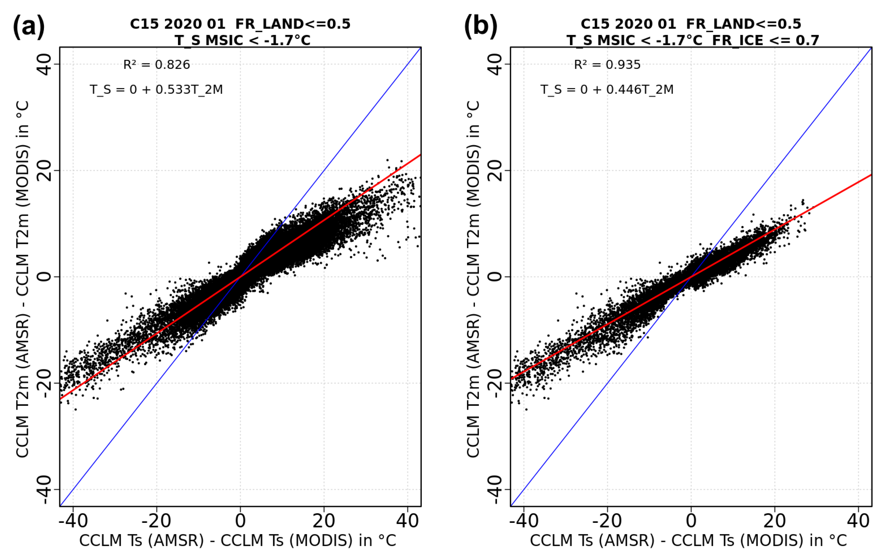
Figure 4 shows two examples of these runs for C15 for January 2020 for (a) all ocean grid points with a surface temperature below 1.7 °C and (b) the same but limited to pixels that suffice a 70% SIC-threshold polynya criteria [37,38]. The temperature criterion excludes open water areas. The results show a clear linear relation between the surface temperature differences and the effect on the 2 m temperatures. For the runs in Figure 4a,b, slopes of 0.53 and 0.45 with respective r2 of 0.83 and 0.94 are found, indicating very good correlations. We investigated this relationship also for polynya grid points that require at least seven contiguous polynya grid points (compare Table 2). Since we cover a very large range in differences between CCLM (AMSR) and CCLM (MODIS), we account for a large range of conditions and seasons.
Here, denotes to the corrected 2 m temperature. While the offset is per default set to be zero, the slope varies between 0.38 and 0.66 depending on the model domain (C15 vs. C05) and applied SIC- and -thresholds to delineate thin-ice areas from thicker ice types (Table 2). All values combined, we get an average slope of around 0.5. This value is assumed to be representative for a wide range of different conditions and hence applied for all cases in the present study. In addition, we evaluated different slope values (0.5 ± 0.05) for their respective effect on retrieved polynya parameters on the Laptev Sea shelf and saw a minor difference of 1 to 3% in the daily polynya area and sea-ice production.
As the dew-point temperature T is used as the quantity for humidity-related fluxes (i.e., latent heat flux and parameterized downwelling longwave radiative flux after [39]) in the thin-ice retrieval, it has to be to adjusted accordingly using the corrected and the initial dew-point depression (; defined as the difference − T):
4. Results
4.1. Case Study from January 2020: Effects of MATA Application
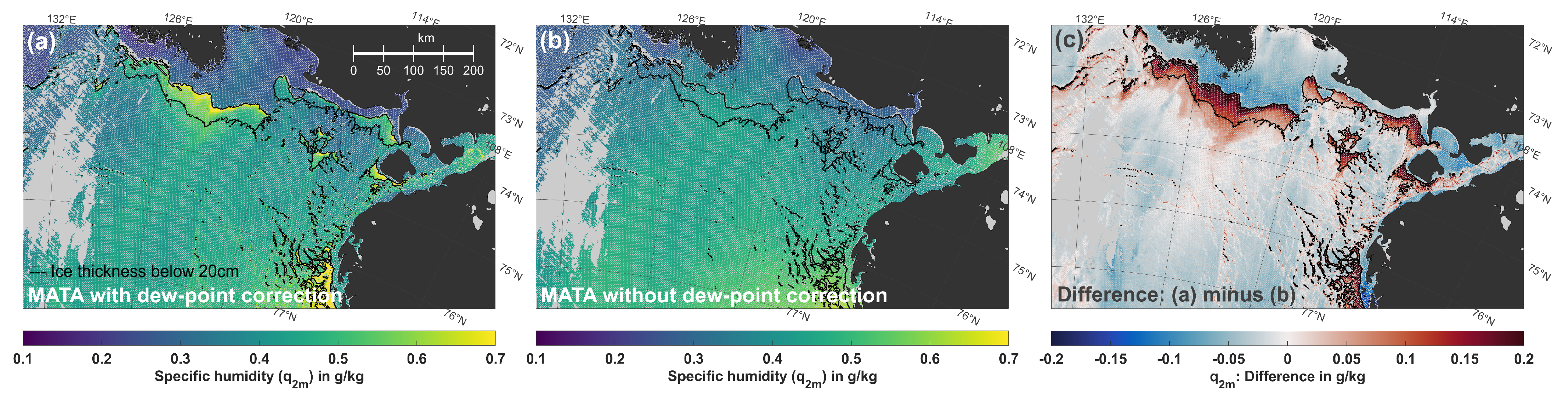
In order to exemplary demonstrate resulting effects of the application of MATA, we here focus on a case study from the Laptev Sea polynya on 2 January 2020 (0425UTC). It first becomes evident from the spatial distributions of the specific humidity at 2 m (; Figure 5), both with and without adjusting the dew-point temperature, that the correction leads to an increase in humidity in proximity of thin ice of around 0.1 to 0.15 g/kg, with some areas exceeding 0.2 g/kg adjacent to the fast-ice edge. These numbers are comparable to in-situ measurements over leads, as reported by [40].
More humid conditions result in increased downward longwave-radiation fluxes that lower the total heat loss to the atmosphere (), due to a humidity-dependency in the parametrization. In turn, the lower atmosphere gets drier than before further offshore, leading to an increase in the total heat loss. Although the magnitude of the change in is not large, the dew-point correction is necessary for physical consistency and hence an integral part of MATA.
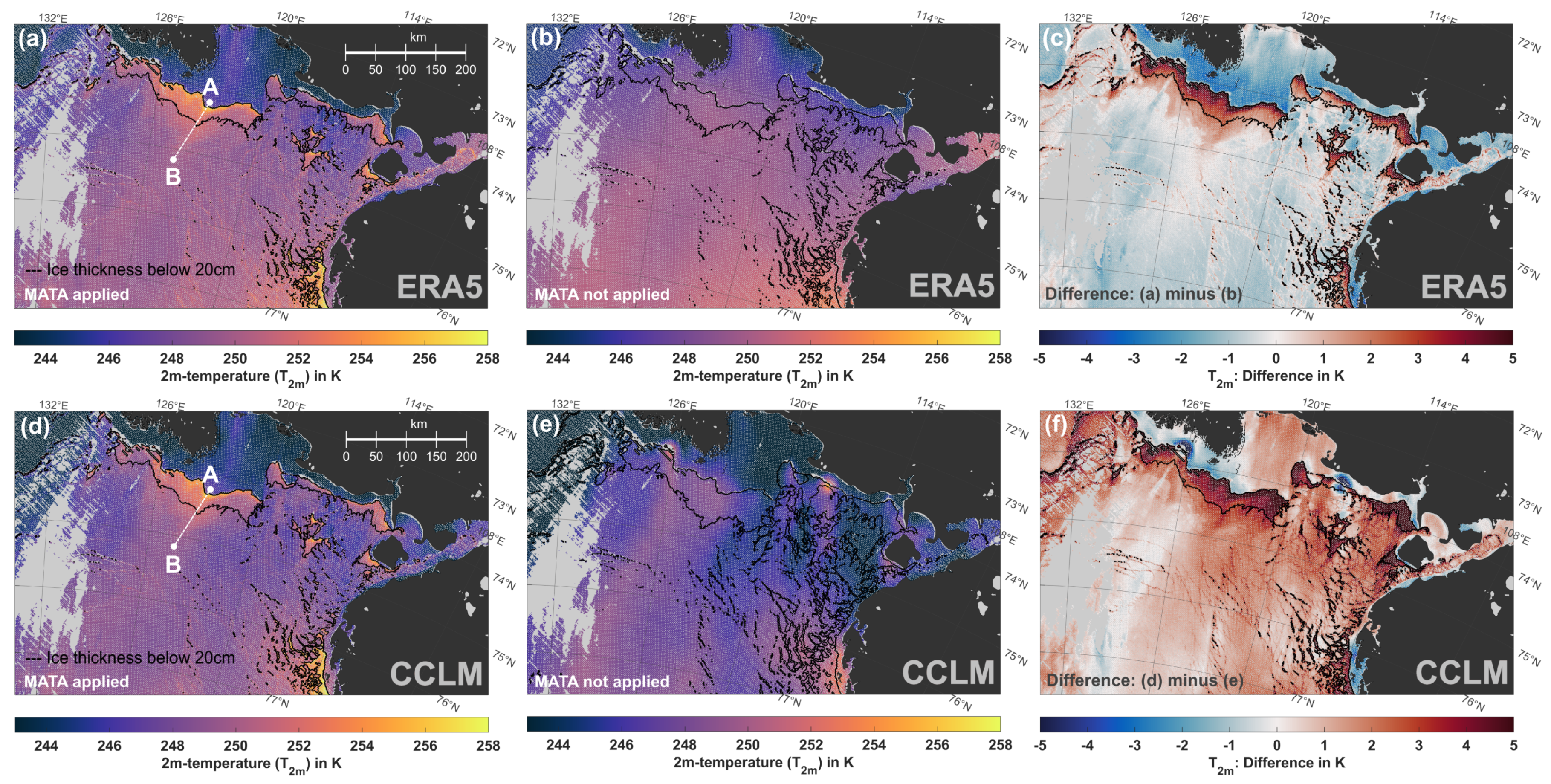
Figure 6 shows the change in 2 m temperature-distributions for the same polynya event on 2 January 2020—therefore focusing on the most obvious and central aspect of MATA. The direct comparison of corrected (panels (a) and (d)) and uncorrected (panels (b) and (e)) temperatures from both ERA5 and CCLM strikingly highlights the imprint of warmer polynya areas adjacent to the cold fast-ice on the lower atmosphere. Absolute differences in these areas range between 1K to more than 5K. Further offshore and above cold fast-ice surfaces, MATA also lowers the 2 m temperature by up to 3–4K. These areas are more widespread in case of ERA5 (Figure 6c and may potentially counteract a warm bias in the original ERA5 data.
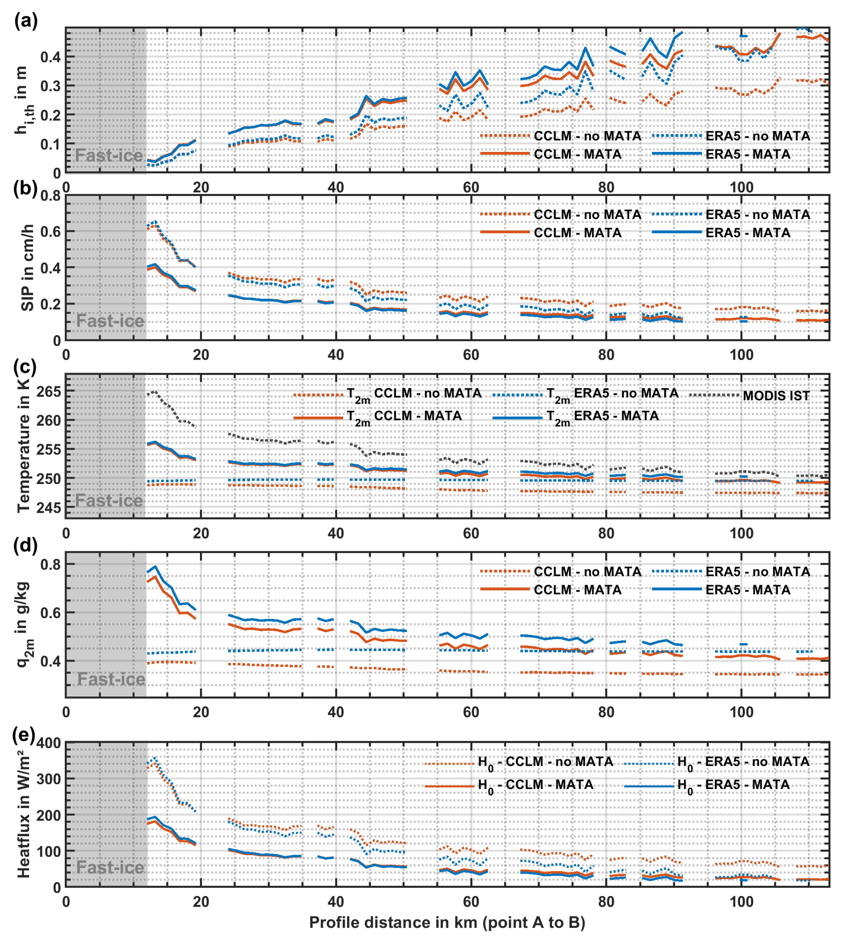
To illustrate the effect of MATA for both the use of CCLM and ERA5 more clearly, Figure 7 shows profiles between two selected points A (74.22°N, 123.09°E; located on fast-ice) and B (75.16°N, 124.48°E; offshore) that cross an active polynya case in the Laptev Sea on 2 January 2020 (04:25UTC). The distance between the two points (compare Figure 6a) is 113 km.
First, we can note that the reanalysis-related differences in ice thickness (panel (a)) and subsequently sea-ice production (SIP; panel (b)) tend to be smaller in those parts with elevated surface temperatures (panel (c)), i.e., the main polynya area with thicknesses below 20 cm. The width of the latter varies depending on the used reanalysis and the use of MATA and ranges between approximately 30 km (MATA cases; CCLM and ERA5 in agreement) and up to 50 km (non-MATA cases; CCLM and ERA5 not in agreement). Within the active polynya zone, SIP reaches values up to 0.4 cm/h (MATA-cases), fading down to about 0.2 cm/h at the 20 cm polynya-threshold. Regarding the MATA-induced adjustment of and , panels (c) and (d) reveal that in case of , the effect of the now included surface-temperature signature leads to a much more realistic temperature profile compared to the initial ’flat’ profiles of both reanalysis. ERA5 temperatures are warmer than their CCLM counterparts both with and without MATA, with the absolute difference being slightly smaller in the MATA case. A similar effect is visible in terms of the specific humidity where we see a noticeable increase in the thinner ice region, as presented in Figure 5.
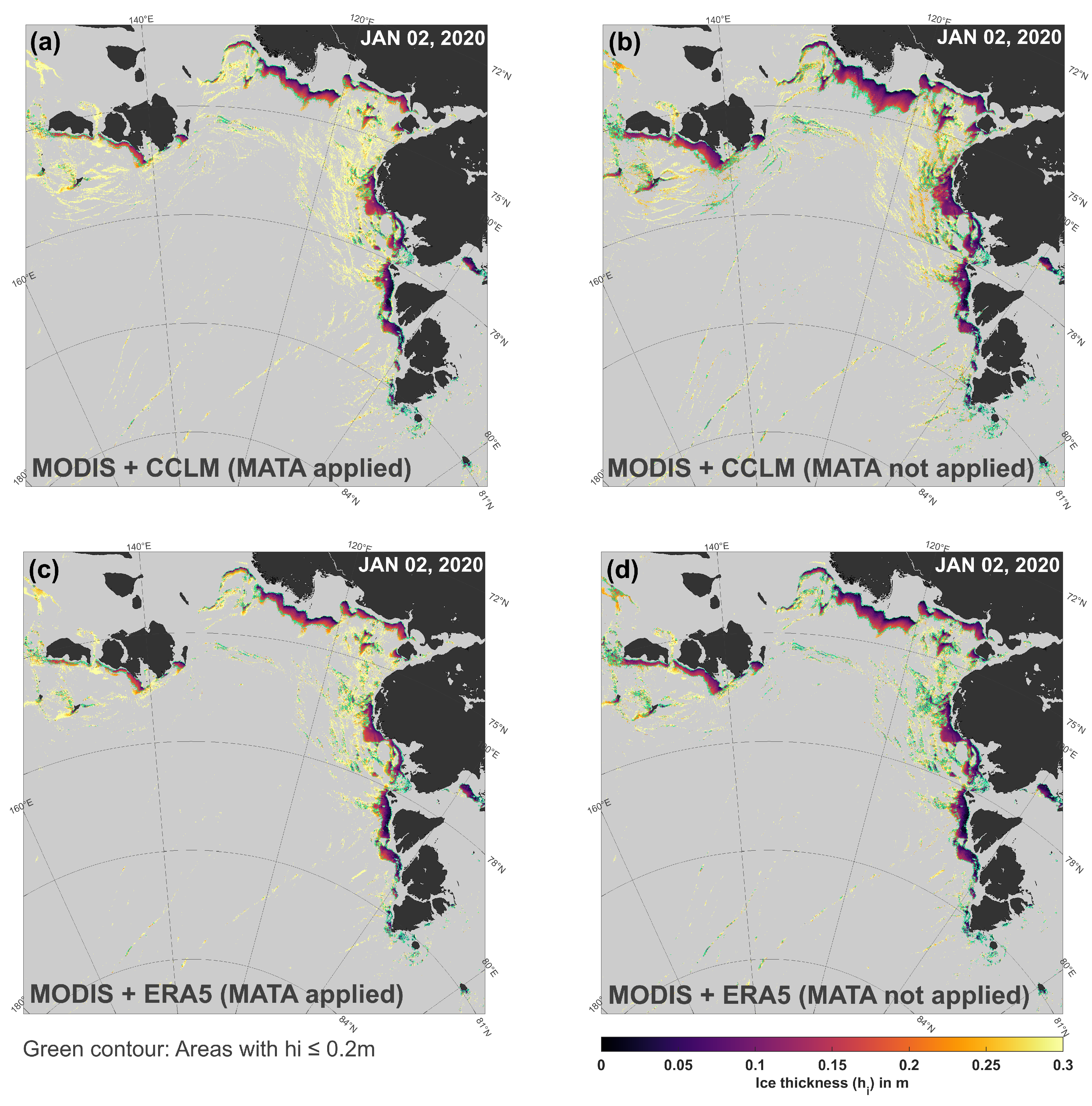
While all MATA-related effects primarily affect the swath-wise calculation of TIT, it is also required to evaluate differences in the daily composites as they are the basis for all long-term investigations of Arctic polynyas. Hence, Figure 8 shows the comparison of MATA and non-MATA daily TIT-composites from 2 January 2020—zoomed in on the same Laptev Sea polynya event as before. Calculated ice thicknesses that use either of the atmospheric data sets (ERA5 and CCLM) are plotted against one another for a clear comparison.
We can easily see how the use of MATA leads to a more congruent distribution of polynyas/thin-ice areas (marked with green outer lines), whereas the non-MATA cases do in parts largely differ from one another—first and foremost in terms of areal extent. This is mainly associated with temperature differences in the respective atmospheric forcing, but differences in the wind field also affect the surface fluxes and thus the computation of TIT. Another interesting observation is that leads are apparently not equally well captured by the ERA5 and CCLM versions, with the CCLM based TIT-distributions featuring more lead-structures than their ERA5 counterparts. Ice thickness estimates in leads mostly range above the 20 cm polynya-threshold.
4.2. Analysis of the 2019/2020 Winter-Season
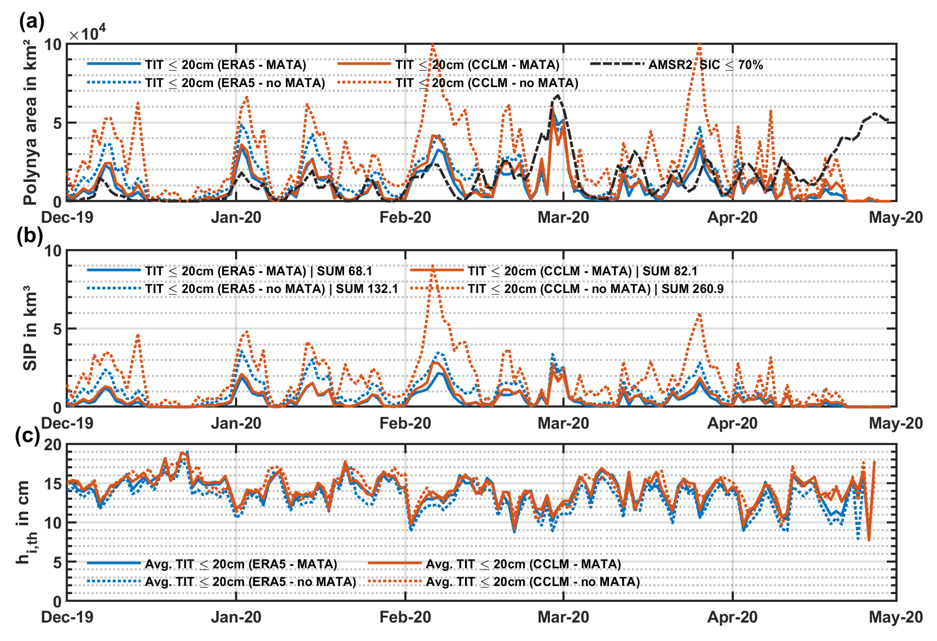
Time series of daily polynya area (POLA, in km2; Figure 9a) and daily accumulated sea-ice production (in km3; Figure 9b) within the Laptev Sea are presented to highlight the wintertime polynya dynamics in 2019/2020 as well as differences among the data set versions (CCLM vs. ERA5; AMSR2 polynya area retrieval based on SIC). As in [2,12], we again set a focus on the Laptev Sea area for this purpose due to its known general importance in a pan-Arctic context (e.g., major source for sea-ice export into the Transpolar Drift system [41,42,43] [among others]) as well as its high activity in 2019/2020.
The latter is well visible in both sub-panels, with more or less extensive thin-ice/open-water areas throughout all months considered. Only in the second half of December 2019 there is a period of about 10 days with hardly any thin-ice/open-water occurrence. The largest thin-ice extent in found around the February-March transition with approximately 55,000 km2 (MODIS based) to 70,000 km2 (AMSR2 based). Interestingly, larger POLA-values from AMSR2, as seen in this case, are less frequently seen in 2019/2020 as the opposite case, with most of the larger polynya events showing higher numbers from MODIS (high agreement between CCLM and ERA5-versions). Other large polynya events show POLA-values of around 30,000 to 40,000 km2. Towards the end of April, we see more apparent differences between the TIT-based MODIS estimates and the SIC-based estimates due to the methodical limitation to nighttime conditions and hence less frequent TIT-estimations with potentially missed polynya observations. Average daily thin-ice thicknesses in the Laptev Sea (Figure 9c) do not differ significantly between the two atmospheric data sets. This is also the case with the effect of the MATA application, where a light increase in thickness can be noted, especially for ERA5.
Likewise as POLA, the daily MODIS-based SIP values show a very high agreement between CCLM and ERA5-versions. There are only two main occasions where CCLM and ERA5 differ more clearly—first an event at the beginning of February (about 0.6 km3 difference; CCLM > ERA5; mainly western Laptev Sea) and then at the already mentioned event at he February-March transition (about 0.5 km3 difference; CCLM < ERA5; western and southern Laptev Sea). Generally, larger polynya events in the Laptev Sea produce roughly 1 to 2 km3 of new ice per day. At the end of April, this sums up to 68.1 km2 (ERA5; 62.5 km3 for DJFM) and 82.1 km3 (CCLM; 74.9 km3 for DJFM) with applied PLF. Without any filtering, these values increase by about 5 to 6%. The overall difference between CCLM and ERA5 SIP-estimates in the Laptev Sea therefore amounts to about 17% in case MATA is applied, which noticeable reduces the initial difference of 49% without MATA (Table 3).
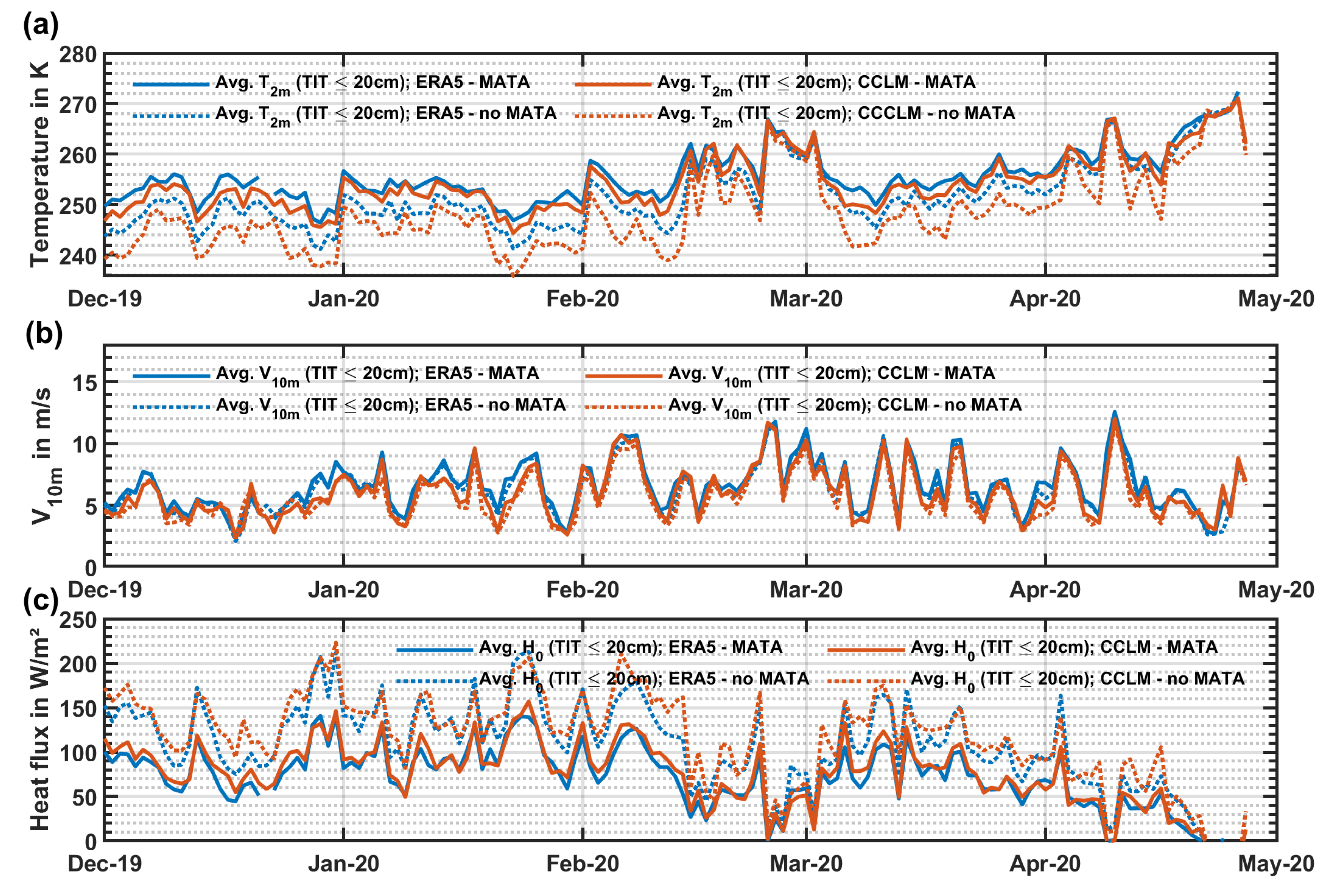
Daily average atmospheric variables (Figure 10) serve to illustrate the effect of MATA on a seasonal timescale. 2 m temperatures over thin ice (≤20 cm) are noticeably adjusted by up to 6–8 K (Figure 10a), which imprints on the derived average sensible heat flux (Figure 10c) and leading to a reduction of the total heat loss to the atmosphere. The 10 m wind speeds are barely influenced by MATA, but it can be noted from Figure 10b that ERA5 wind speeds overall exceed those of CCLM, which has an additional effect on observed SIP differences.
Compared to the SIP in other winters, the season of 2019/2020 lies slightly above previously reported average values for the Laptev Sea domain [2,44]. Adjacent seas (East Siberian Sea, Kara Sea) in the eastern Arctic show a similar behaviour in this particular winter, while a closer look at other polynya regions across the Arctic (Table 3) reveals a more diverse picture. Especially polynyas in the western Arctic, such as the North Water polynya between Greenland and Canada, were noticeable less active in 2019/2020 when compared to preceding winter seasons (even when taking the 2002/2003 to 2017/2018 standard deviation into account). One reason for this contrast could be the extremely stable polar vortex in the winter 2019/2020, which appeared in concert with an record-high positive phase of the Arctic Oscillation (AO) between January and March 2020 [45] and unprecedented warming events over the Siberian Seas [46]. The resulting increase in sea-ice drift-speed and low (initial) ice thicknesses in the Siberian seas are a likely explanation for the enhanced polynya activity on the East Siberian and Laptev Sea shelves as well as reported slightly increased fracturing along the Transpolar Drift [47,48].
Regarding the application of MATA, we see that the overall difference between CCLM and ERA5 is reduced from 49% to 23%, with certain regions showing larger decreases than others (e.g., Chukchi Sea, East-Siberian Sea, Severnaya Zemlya). Table 3 further reveals that the individual effect of MATA per region noticeably differs between CCLM (SIP reduced by −23% to −75%) and ERA5 (SIP reduced by −21% to −55%), which is supposedly related to the initially larger deviations in terms of 2 m temperatures distributions (as shown in Figure 10a for the Laptev Sea).
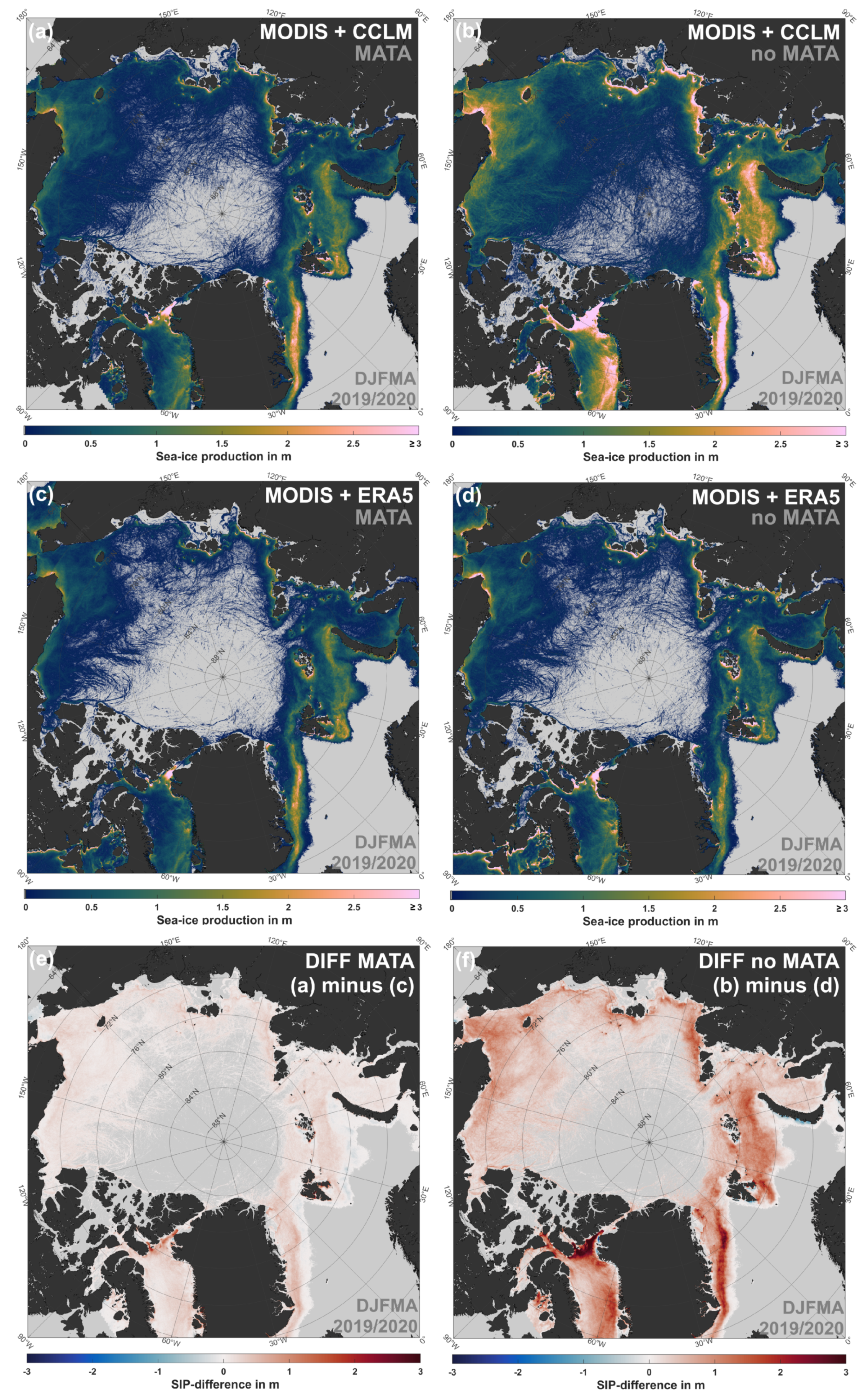
In order to highlight spatial differences among the utilization of different atmospheric data sets (CCLM ((a) and (b)) and ERA5 ((c) and (d))) on a pan-Arctic scale, Figure 11 shows overviews of accumulated sea-ice production (in m/winter) for the extended winter-season from December 2019 to April 2020, before and after application of MATA. Maps indicating the respective difference between CCLM and ERA5 are presented in Figure 11e,f. Overall, we see broad similarities between the CCLM and ERA5-versions through MATA, both in terms of the general spatial distribution of increased SIP and in terms of magnitude. This imprints on generally low differences throughout the Arctic, which is in stark contrast to larger differences without utilizing MATA. However, a closer look reveals that especially the CCLM based distribution shows elevated SIP values of typically lower than 1 m/winter per individual pixel-location further offshore (e.g., central Laptev Sea, East Siberian Sea, along the Transpolar Drift and within the Beaufort Gyre region), which are seemingly related to enhanced lead-occurrences.
While some of these areas are also (less clearly) visible in the ERA5 distribution, the CCLM distribution more resembles the long-term distribution of leads as presented in [3] or [4]. However, we have to note that these SIP values/distributions are solely based on TIT ≤0.2 m, thereby seemingly representing the minority of leads in the central Arctic Ocean (compare Figure 2 in Section 3) which more commonly seem to exceed our fixed thin-ice threshold of 20cm. Another interesting difference can be seen for the NOW polynya, where the SIP using the CCLM data is much larger compared to ERA5 (compare Figure 11e and Table 3). Here the wind field is largely determined by the channeling effect of the topography of Nares Strait, which is not adequately represented in the ERA5 data [49].
5. Discussion and Conclusions
Our results demonstrate the wide-ranging positive effect of adding the MATA algorithm to the thin-ice thickness retrieval based on MODIS satellite data. First and foremost, the primary aim of increasing the comparability between different atmospheric data sets that force the retrieval could be achieved with success. In particular, too cold model-based 2 m temperatures in proximity of warmer ice or ocean areas, as indicated by MODIS IST, would lead to an overestimation of POLA and SIP. Our proposed MATA method leads to an adequate adjustment to account for associated changes in atmospheric heat fluxes. The method definitely improves previous versions of MODIS-based thin-ice thickness retrievals.
While the development of the MATA method is purely model-based (covering a wide range of atmospheric conditions), the application of MATA needs no modelling and can be applied by all studies using TIR data in combination with atmospheric reanalyses. Among the parts of MATA that offer room for future improvement is the currently fixed slope value of 0.5, which could in principle vary depending on different regional environmental conditions. As our chosen value is based on both pan-Arctic as well as two regional domains with a wide range of different conditions, we consider it to be generally applicable to other use cases. In the course of development, we saw only a minor effect through varying the slope value (0.5 ± 0.05), with differences of 1–3% in the daily POLA and SIP on the Laptev Sea shelf.
Another obvious topic for discussion is the meanwhile well-known warm bias ( of ERA5 and ERA Interim) over Arctic sea-ice. Quite recently, the study by [50] presented a collective overview based on buoy comparisons across the Arctic Ocean between 2010 and 2020. For ERA5, they found a warm bias of 2.34 ± 3.22 K, which implies generally underestimated heat fluxes during the cold and dark winter months—our period of interest. In previous MODIS-based studies, this effect caused an additional uncertainty for derived ice thicknesses and sea-ice production estimates. Through MATA, we noticed a two-sided effect of our temperature adjustment (as indicated in Section 3 and Section 4): In addition, increased 2 m temperatures above/near polynyas and leads, areas with thicker ice were also corrected in the opposite direction, thereby compensating the war m bias in the ERA5 data set to some extent.
Along those lines and together with other newly introduced modifications (such as changes in the cloud-filtering and the addition of classified leads), we note that the absolute numbers for POLA and SIP are lower than earlier MODIS-based estimates in [12] or [2]. This is not surprising in case of thin ice, given that the increase in 2 m temperatures through MATA causes a lower difference to the corresponding IST as well as an increase in humidity (through the dew-point temperature adjustment). The latter imprints on both the parameterized downward-longwave radiation and the latent heat flux, with the effect of a further reduced net energy flux to the atmosphere that leads to thicker ice estimates and lower ice formation rates. A future long-term comparison (including the complete MODIS data record) is required to give a final verdict on the exact magnitude of differences.
Regarding the lead-related changes to the TIT retrieval, in particular the inclusion of the ArcLead-product by [4] as a measure for lead locations in the daily TIT composites, we certainly re-introduce some potential draw-backs or error-sources that were in parts already addressed in earlier studies. These include for instance the exclusion of a spatial thin-ice interpolation scheme [35] and the risk of analysing potentially cloud-influenced (thin-ice) pixels with a low daily persistence, given they are classified as a lead in the ArcLead-product. On the other hand, in case of non-cloud-influenced cases, these additional low-persistence pixels can give valuable information on the spatial thin-ice distribution in a given region (including characteristic patterns) that would have been omitted in previous MODIS TIT-based studies or other similar investigations using passive microwave data, e.g., [9,10,51].
To conclude, we consider the presented changes and additions to the satellite-based thin-ice thickness retrieval as being vital steps towards an improved characterisation of ice thicknesses in both polynyas and leads. Together with advances through novel machine-learning based cloud-detection algorithms [52] and the availability of thermal-infrared data from more recent satellite systems (such as Sentinel-3’s SLSTR), these are excellent prospects for future TIR-based thin-ice investigations in the Arctic and Antarctic seas.
Author Contributions
Conceptualization, A.P. and G.H.; Data curation, A.P., L.S. and S.W.; Formal analysis, A.P.; Funding acquisition, G.H.; Methodology, A.P., G.H. and L.S.; Software, A.P. and S.W.; Visualization, A.P. and L.S.; Writing—original draft, A.P. and G.H.; Writing—review and editing, A.P., G.H., L.S. and S.W. All authors have read and agreed to the published version of the manuscript.
Funding
This work was funded by the Federal Ministry of Education and Research (Bundesministerium für Bildung und Forschung—BMBF) under Grant 03F0776D (“CATS”) and 03F0831C (“CATS-Synthesis”). The publication was funded by the Open Access Fund of the University of Trier and the German Research Foundation (DFG) within the Open Access Publishing funding program.
Data Availability Statement
Data are available on request from the authors. After processing of the MxD29 archive (winter months from 2002 to 2021), data will be made available on the public data repository PANGAEA.
Acknowledgments
The National Snow and Ice Data Center (NSIDC) as well as the European Center for Medium Range Weather Forecasts (ECMWF) are kindly acknowledged for providing the MODIS MxD29 sea-ice product (https://n5eil01u.ecs.nsidc.org/ (last accessed on 14 March 2022)) and the ERA5 atmospheric reanalysis data free of charge. Thanks go to the CLM Community and the German Meteorological Service for providing the basic COSMO-CLM model. This work used resources of the Deutsches Klimarechenzentrum (DKRZ) granted by its Scientific Steering Committee (WLA) under project ID 474. This study mainly uses scientific colour maps after [53]. We thank Rich Pawlowicz for the mapping package (https://www.eoas.ubc.ca/~rich/map.html (last accessed on 14 March 2022)) and the kind technical support.
Conflicts of Interest
The authors declare no conflict of interest.
References
- Smith, S.D.; Muench, R.D.; Pease, C.H. Polynyas and leads: An overview of physical processes and environment. J. Geophys. Res. 1990, 95, 9461–9479. [Google Scholar] [CrossRef]
- Preußer, A.; Ohshima, K.I.; Iwamoto, K.; Willmes, S.; Heinemann, G. Retrieval of Wintertime sea-ice Production in Arctic Polynyas Using Thermal Infrared and Passive Microwave Remote Sensing Data. J. Geophys. Res. Ocean. 2019, 124, 5503–5528. [Google Scholar] [CrossRef] [Green Version]
- Willmes, S.; Heinemann, G. Sea-Ice Wintertime Lead Frequencies and Regional Characteristics in the Arctic, 2003–2015. Remote Sens. 2016, 8, 4. [Google Scholar] [CrossRef] [Green Version]
- Reiser, F.; Willmes, S.; Heinemann, G. A New Algorithm for Daily sea-ice Lead Identification in the Arctic and Antarctic Winter from Thermal-Infrared Satellite Imagery. Remote Sens. 2020, 12, 1957. [Google Scholar] [CrossRef]
- Steffen, K. Ice conditions of an Arctic polynya: North Water in winter. J. Glaciol. 1986, 32, 383–390. [Google Scholar] [CrossRef] [Green Version]
- Steffen, K.; Maslanik, J.A. Comparison of Nimbus 7 scanning multichannel microwave radiometer radiance and derived sea-ice concentrations with Landsat imagery for the north water area of Baffin Bay. J. Geophys. Res. Ocean. 1988, 93, 10769–10781. [Google Scholar] [CrossRef]
- Yu, Y.; Rothrock, D. Thin ice thickness from satellite thermal imagery. J. Geophys. Res. Ocean. 1996, 101, 25753–25766. [Google Scholar] [CrossRef]
- Yu, Y.; Lindsay, R. Comparison of thin ice thickness distributions derived from RADARSAT Geophysical Processor System and Advanced Very High Resolution Radiometer data sets. J. Geophys. Res. 2003, 108, 3387. [Google Scholar] [CrossRef]
- Tamura, T.; Ohshima, K.I. Mapping of sea-ice production in the Arctic coastal polynyas. J. Geophys. Res. 2011, 116, C07030. [Google Scholar] [CrossRef]
- Iwamoto, K.; Ohshima, K.I.; Tamura, T. Improved mapping of sea-ice production in the Arctic Ocean using AMSR-E thin ice thickness algorithm. J. Geophys. Res. Ocean. 2014, 119, 3574–3594. [Google Scholar] [CrossRef]
- Paul, S.; Willmes, S.; Heinemann, G. Long-term coastal-polynya dynamics in the Southern Weddell Sea from MODIS thermal-infrared imagery. Cryosphere 2015, 9, 2027–2041. [Google Scholar] [CrossRef] [Green Version]
- Preußer, A.; Heinemann, G.; Willmes, S.; Paul, S. Circumpolar polynya regions and ice production in the Arctic: Results from MODIS thermal infrared imagery from 2002/2003 to 2014/2015 with a regional focus on the Laptev Sea. Cryosphere 2016, 10, 3021–3042. [Google Scholar] [CrossRef] [Green Version]
- Dee, D.P.; Uppala, S.M.; Simmons, A.J.; Berrisford, P.; Poli, P.; Kobayashi, S.; Andrae, U.; Balmaseda, M.A.; Balsamo, G.; Bauer, P.; et al. The ERA-Interim reanalysis: Configuration and performance of the data assimilation system. Q. J. R. Meteorol. Soc. 2011, 137, 553–597. [Google Scholar] [CrossRef]
- Hersbach, H.; Bell, B.; Berrisford, P.; Hirahara, S.; Horányi, A.; Muñoz-Sabater, J.; Nicolas, J.; Peubey, C.; Radu, R.; Schepers, D.; et al. The ERA5 global reanalysis. Q. J. R. Meteorol. Soc. 2020, 146, 1999–2049. [Google Scholar] [CrossRef]
- Jakobsson, M.; Mayer, L.; Coakley, B.; Dowdeswell, J.A.; Forbes, S.; Fridman, B.; Hodnesdal, H.; Noormets, R.; Pedersen, R.; Rebesco, M.; et al. The international bathymetric chart of the Arctic Ocean (IBCAO) version 3.0. Geophys. Res. Lett. 2012, 39, 176. [Google Scholar] [CrossRef] [Green Version]
- Nielsen-Englyst, P.; Høyer, J.L.; Madsen, K.S.; Tonboe, R.; Dybkjær, G.; Alerskans, E. In situ observed relationships between snow and ice surface skin temperatures and 2 m air temperatures in the Arctic. Cryosphere 2019, 13, 1005–1024. [Google Scholar] [CrossRef] [Green Version]
- Nielsen-Englyst, P.; Høyer, J.L.; Madsen, K.S.; Tonboe, R.T.; Dybkjær, G.; Skarpalezos, S. Deriving Arctic 2 m air temperatures over snow and ice from satellite surface temperature measurements. Cryosphere 2021, 15, 3035–3057. [Google Scholar] [CrossRef]
- Ackerman, S.; Frey, R.; Strabala, K.; Liu, Y.; Gumley, L.; Baum, B.; Menzel, P. Discriminating Clear-Sky from Cloud with MODIS Algorithm Theoretical Basis Document (MOD35) Version 6.1; Technical Report; MODIS Cloud Mask Team, Cooperative Institute for Meteorological Satellite Studies, University of Wisconsin: Madison, WI, USA, 2010. [Google Scholar]
- Hall, D.; Key, J.; Casey, K.; Riggs, G.; Cavalieri, D. sea-ice surface temperature product from MODIS. Geosci. Remote Sens. IEEE Trans. 2004, 42, 1076–1087. [Google Scholar] [CrossRef]
- Riggs, G.; Hall, D. MODIS sea-ice Products User Guide to Collection 6; National Snow and Ice Data Center, University of Colorado: Boulder, CO, USA, 2015. [Google Scholar]
- Spreen, G.; Kaleschke, L.; Heygster, G. Sea-ice remote sensing using AMSR-E 89 GHz channels. J. Geophys. Res. 2008, 113, C02S03. [Google Scholar] [CrossRef] [Green Version]
- Gutjahr, O.; Heinemann, G.; Preußer, A.; Willmes, S.; Drüe, C. Quantification of ice production in Laptev Sea polynyas and its sensitivity to thin-ice parameterizations in a regional climate model. Cryosphere 2016, 10, 2999–3019. [Google Scholar] [CrossRef] [Green Version]
- Heinemann, G.; Willmes, S.; Schefczyk, L.; Makshtas, A.; Kustov, V.; Makhotina, I. Observations and Simulations of Meteorological Conditions over Arctic Thick sea-ice in Late Winter during the Transarktika 2019 Expedition. Atmosphere 2021, 12, 174. [Google Scholar] [CrossRef]
- Sedlar, J.; Tjernström, M.; Rinke, A.; Orr, A.; Cassano, J.; Fettweis, X.; Heinemann, G.; Seefeldt, M.; Solomon, A.; Matthes, H.; et al. Confronting Arctic Troposphere, Clouds, and Surface Energy Budget Representations in Regional Climate Models With Observations. J. Geophys. Res. Atmos. 2020, 125, e2019JD031783. [Google Scholar] [CrossRef]
- Inoue, J.; Sato, K.; Rinke, A.; Cassano, J.J.; Fettweis, X.; Heinemann, G.; Matthes, H.; Orr, A.; Phillips, T.; Seefeldt, M.; et al. Clouds and Radiation Processes in Regional Climate Models Evaluated Using Observations Over the Ice-free Arctic Ocean. J. Geophys. Res. Atmos. 2021, 126, e2020JD033904. [Google Scholar] [CrossRef]
- Zhang, J.; Rothrock, D.A. Modeling Global sea-ice with a Thickness and Enthalpy Distribution Model in Generalized Curvilinear Coordinates. Mon. Weather Rev. 2003, 131, 845–861. [Google Scholar] [CrossRef] [Green Version]
- Lavergne, T.; Sørensen, A.M.; Kern, S.; Tonboe, R.; Notz, D.; Aaboe, S.; Bell, L.; Dybkjær, G.; Eastwood, S.; Gabarro, C.; et al. Version 2 of the EUMETSAT OSI SAF and ESA CCI sea-ice concentration climate data records. Cryosphere 2019, 13, 49–78. [Google Scholar] [CrossRef] [Green Version]
- Donlon, C.J.; Martin, M.; Stark, J.; Roberts-Jones, J.; Fiedler, E.; Wimmer, W. The Operational Sea Surface Temperature and sea-ice Analysis (OSTIA) system. Remote Sens. Environ. 2012, 116, 140–158. [Google Scholar] [CrossRef]
- Renfrew, I.A.; Barrell, C.; Elvidge, A.D.; Brooke, J.K.; Duscha, C.; King, J.C.; Kristiansen, J.; Cope, T.L.; Moore, G.W.K.; Pickart, R.S.; et al. An evaluation of surface meteorology and fluxes over the Iceland and Greenland Seas in ERA5 reanalysis: The impact of sea-ice distribution. Q. J. R. Meteorol. Soc. 2021, 147, 691–712. [Google Scholar] [CrossRef]
- Batrak, Y.; Müller, M. On the warm bias in atmospheric reanalyses induced by the missing snow over Arctic sea-ice. Nat. Commun. 2019, 10, 4170. [Google Scholar] [CrossRef]
- Adams, S.; Willmes, S.; Schroeder, D.; Heinemann, G.; Bauer, M.; Krumpen, T. Improvement and sensitivity analysis of thermal thin-ice retrievals. IEEE Trans. Geosci. Remote Sens. 2013, 51, 3306–3318. [Google Scholar] [CrossRef] [Green Version]
- WMO; OMM; BMO. WMO Sea-Ice Nomenclature; Edition 1970–2014 259; WMO/OMM/BMO: Geneva, Switzerland, 2014. [Google Scholar]
- Launiainen, J.; Vihma, T. Derivation of turbulent surface fluxes—An iterative flux-profile method allowing arbitrary observing heights. Environ. Softw. 1990, 5, 113–124. [Google Scholar] [CrossRef]
- Preußer, A.; Heinemann, G.; Willmes, S.; Paul, S. Multi-Decadal Variability of Polynya Characteristics and Ice Production in the North Water Polynya by Means of Passive Microwave and Thermal Infrared Satellite Imagery. Remote Sens. 2015, 7, 15844–15867. [Google Scholar] [CrossRef] [Green Version]
- Paul, S.; Willmes, S.; Gutjahr, O.; Preußer, A.; Heinemann, G. Spatial Feature Reconstruction of Cloud-Covered Areas in Daily MODIS Composites. Remote Sens. 2015, 7, 5042–5056. [Google Scholar] [CrossRef] [Green Version]
- Willmes, S.; Krumpen, T.; Adams, S.; Rabenstein, L.; Haas, C.; Hoelemann, J.; Hendricks, S.; Heinemann, G. Cross-validation of polynya monitoring methods from multisensor satellite and airborne data: A case study for the Laptev Sea. Can. J. Remote Sens. 2010, 36, S196–S210. [Google Scholar] [CrossRef]
- Massom, R.A.; Harris, P.; Michael, K.J.; Potter, M. The distribution and formative processes of latent-heat polynyas in East Antarctica. Ann. Glaciol. 1998, 27, 420–426. [Google Scholar] [CrossRef] [Green Version]
- Adams, S.; Willmes, S.; Heinemann, G.; Rozman, P.; Timmermann, R.; Schröder, D. Evaluation of simulated sea-ice concentrations from sea-ice/ ocean models using satellite data and polynya classification methods. Polar Res. 2011, 30, 7124. [Google Scholar] [CrossRef]
- Jin, X.; Barber, D.; Papakyriakou, T. A new clear-sky downward longwave radiative flux parameterization for Arctic areas based on rawinsonde data. J. Geophys. Res. 2006, 111, D24104. [Google Scholar] [CrossRef] [Green Version]
- Tetzlaff, A.; Lüpkes, C.; Hartmann, J. Aircraft-based observations of atmospheric boundary-layer modification over Arctic leads. Q. J. R. Meteorol. Soc. 2015, 141, 2839–2856. [Google Scholar] [CrossRef]
- Dethleff, D.; Loewe, P.; Kleine, E. The Laptev Sea flaw lead—Detailed investigation on ice formation and export during 1991/1992 winter season. Cold Reg. Sci. Technol. 1998, 27, 225–243. [Google Scholar] [CrossRef]
- Itkin, P.; Krumpen, T. Winter sea-ice export from the Laptev Sea preconditions the local summer sea-ice cover and fast ice decay. Cryosphere 2017, 11, 2383–2391. [Google Scholar] [CrossRef] [Green Version]
- Krumpen, T.; Belter, H.J.; Boetius, A.; Damm, E.; Haas, C.; Hendricks, S.; Nicolaus, M.; Nöthig, E.M.; Paul, S.; Peeken, I.; et al. Arctic warming interrupts the Transpolar Drift and affects long-range transport of sea-ice and ice-rafted matter. Sci. Rep. 2019, 9, 5459. [Google Scholar] [CrossRef] [Green Version]
- Willmes, S.; Adams, S.; Schröder, D.; Heinemann, G. Spatio-temporal variability of polynya dynamics and ice production in the Laptev Sea between the winters of 1979/80 and 2007/08. Polar Res. 2011, 30, 16. [Google Scholar] [CrossRef]
- Lawrence, Z.D.; Perlwitz, J.; Butler, A.H.; Manney, G.L.; Newman, P.A.; Lee, S.H.; Nash, E.R. The Remarkably Strong Arctic Stratospheric Polar Vortex of Winter 2020: Links to Record-Breaking Arctic Oscillation and Ozone Loss. J. Geophys. Res. Atmos. 2020, 125, e2020JD033271. [Google Scholar] [CrossRef]
- Rinke, A.; Cassano, J.J.; Cassano, E.N.; Jaiser, R.; Handorf, D. Meteorological conditions during the MOSAiC expedition: Normal or anomalous? Elem. Sci. Anthr. 2021, 9, 00023. [Google Scholar] [CrossRef]
- Krumpen, T.; Birrien, F.; Kauker, F.; Rackow, T.; von Albedyll, L.; Angelopoulos, M.; Belter, H.J.; Bessonov, V.; Damm, E.; Dethloff, K.; et al. The MOSAiC ice floe: Sediment-laden survivor from the Siberian shelf. Cryosphere 2020, 14, 2173–2187. [Google Scholar] [CrossRef]
- Krumpen, T.; von Albedyll, L.; Goessling, H.F.; Hendricks, S.; Juhls, B.; Spreen, G.; Willmes, S.; Belter, H.J.; Dethloff, K.; Haas, C.; et al. MOSAiC drift expedition from October 2019 to July 2020: Sea-ice conditions from space and comparison with previous years. Cryosphere 2021, 15, 3897–3920. [Google Scholar] [CrossRef]
- Kohnemann, S.H.; Heinemann, G. A climatology of wintertime low-level jets in Nares Strait. Polar Res. 2021, 40, 3622. [Google Scholar] [CrossRef]
- Yu, Y.; Xiao, W.; Zhang, Z.; Cheng, X.; Hui, F.; Zhao, J. Evaluation of 2-m Air Temperature and Surface Temperature from ERA5 and ERA-I Using Buoy Observations in the Arctic during 2010–2020. Remote Sens. 2021, 13, 2813. [Google Scholar] [CrossRef]
- Ohshima, K.I.; Tamaru, N.; Kashiwase, H.; Nihashi, S.; Nakata, K.; Iwamoto, K. Estimation of sea-ice Production in the Bering Sea From AMSR-E and AMSR2 Data, With Special Emphasis on the Anadyr Polynya. J. Geophys. Res. Ocean. 2020, 125, e2019JC016023. [Google Scholar] [CrossRef]
- Paul, S.; Huntemann, M. Improved machine-learning-based open-water–sea-ice–cloud discrimination over wintertime Antarctic sea-ice using MODIS thermal-infrared imagery. Cryosphere 2021, 15, 1551–1565. [Google Scholar] [CrossRef]
- Crameri, F.; Shephard, G.E.; Heron, P.J. The misuse of colour in science communication. Nat. Commun. 2020, 11, 5444. [Google Scholar] [CrossRef]
Figure 1.
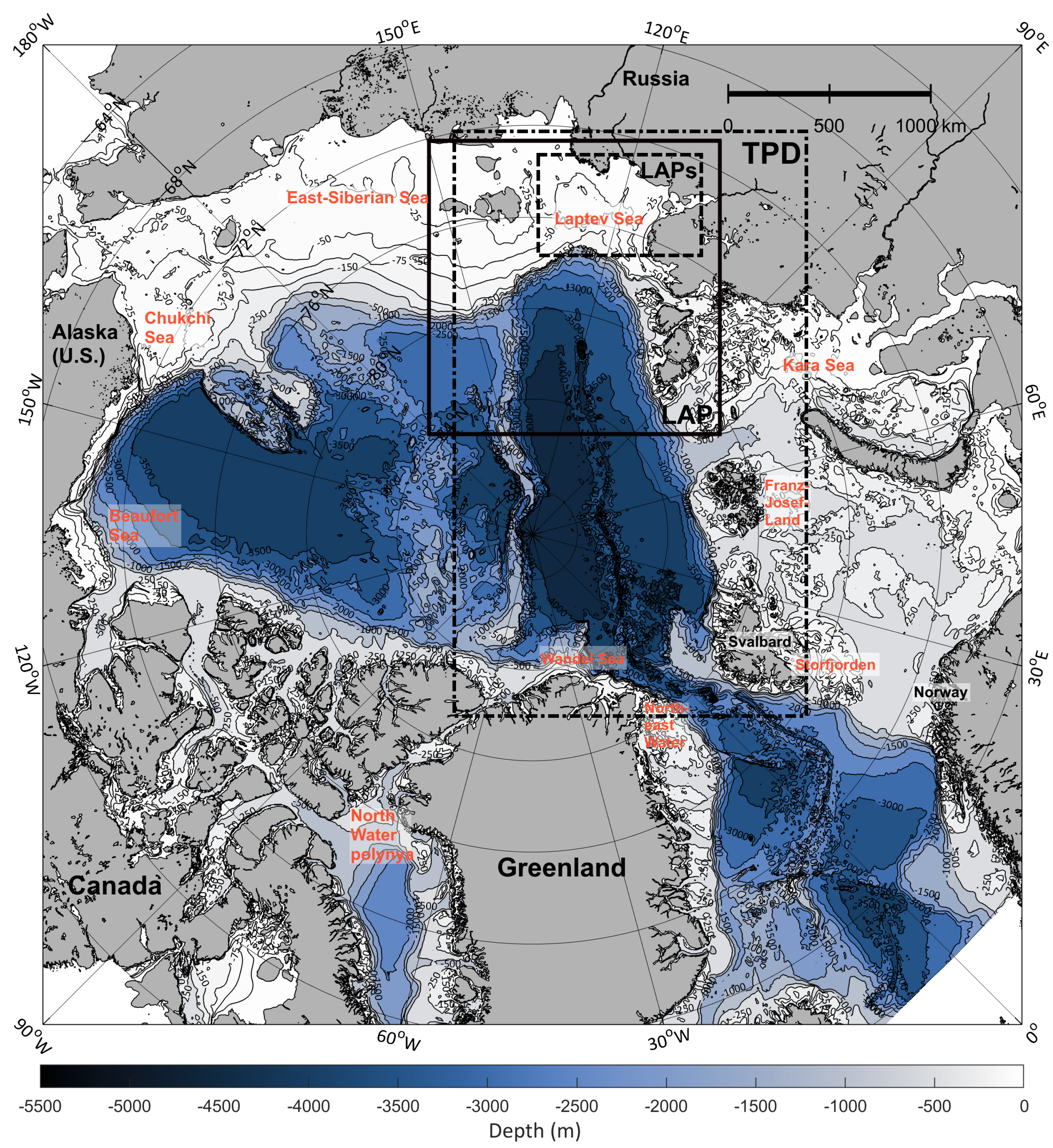
Overview map of the Arctic Ocean and adjacent seas, with color-levels indicating ocean depth (in m) according to IBCAO (v3) bathymetric data [15]. Subset areas for case studies in later figures are depicted with black frames, showing the Transpolar Drift (TPD; dash-dotted), the wider Laptev Sea (LAP; solid) and a southern Laptev Sea close-up (LAPs; dashed).
Figure 1.
Overview map of the Arctic Ocean and adjacent seas, with color-levels indicating ocean depth (in m) according to IBCAO (v3) bathymetric data [15]. Subset areas for case studies in later figures are depicted with black frames, showing the Transpolar Drift (TPD; dash-dotted), the wider Laptev Sea (LAP; solid) and a southern Laptev Sea close-up (LAPs; dashed).

Figure 2.
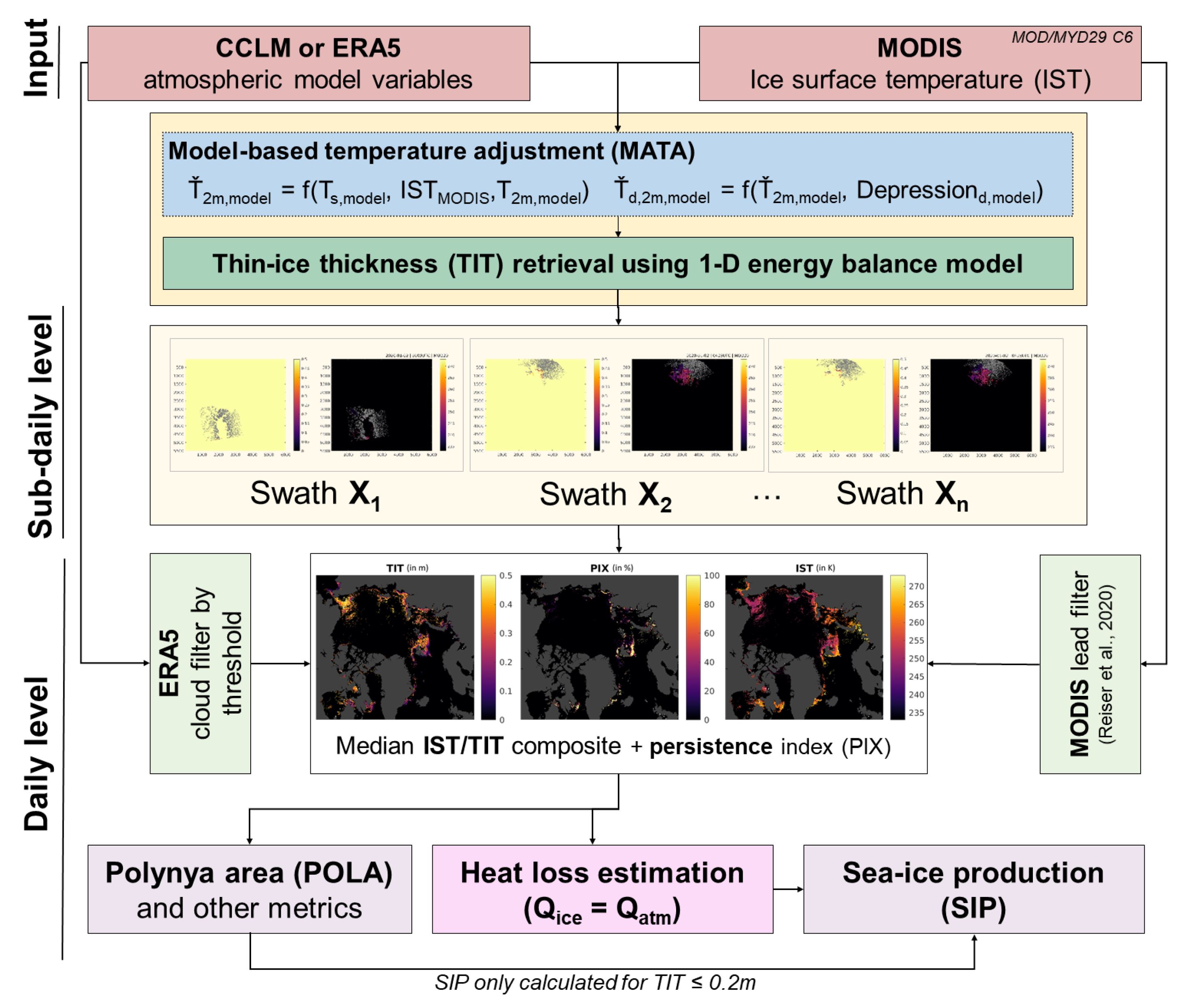
The thin-ice thickness (TIT) retrieval using MODIS ice-surface temperature data with atmospheric variables from COSMO CLM or ECMWF ERA5 reanalysis. The newly added model-assisted temperature adjustment scheme (MATA) is indicated in blue.
Figure 2.
The thin-ice thickness (TIT) retrieval using MODIS ice-surface temperature data with atmospheric variables from COSMO CLM or ECMWF ERA5 reanalysis. The newly added model-assisted temperature adjustment scheme (MATA) is indicated in blue.

Figure 3.
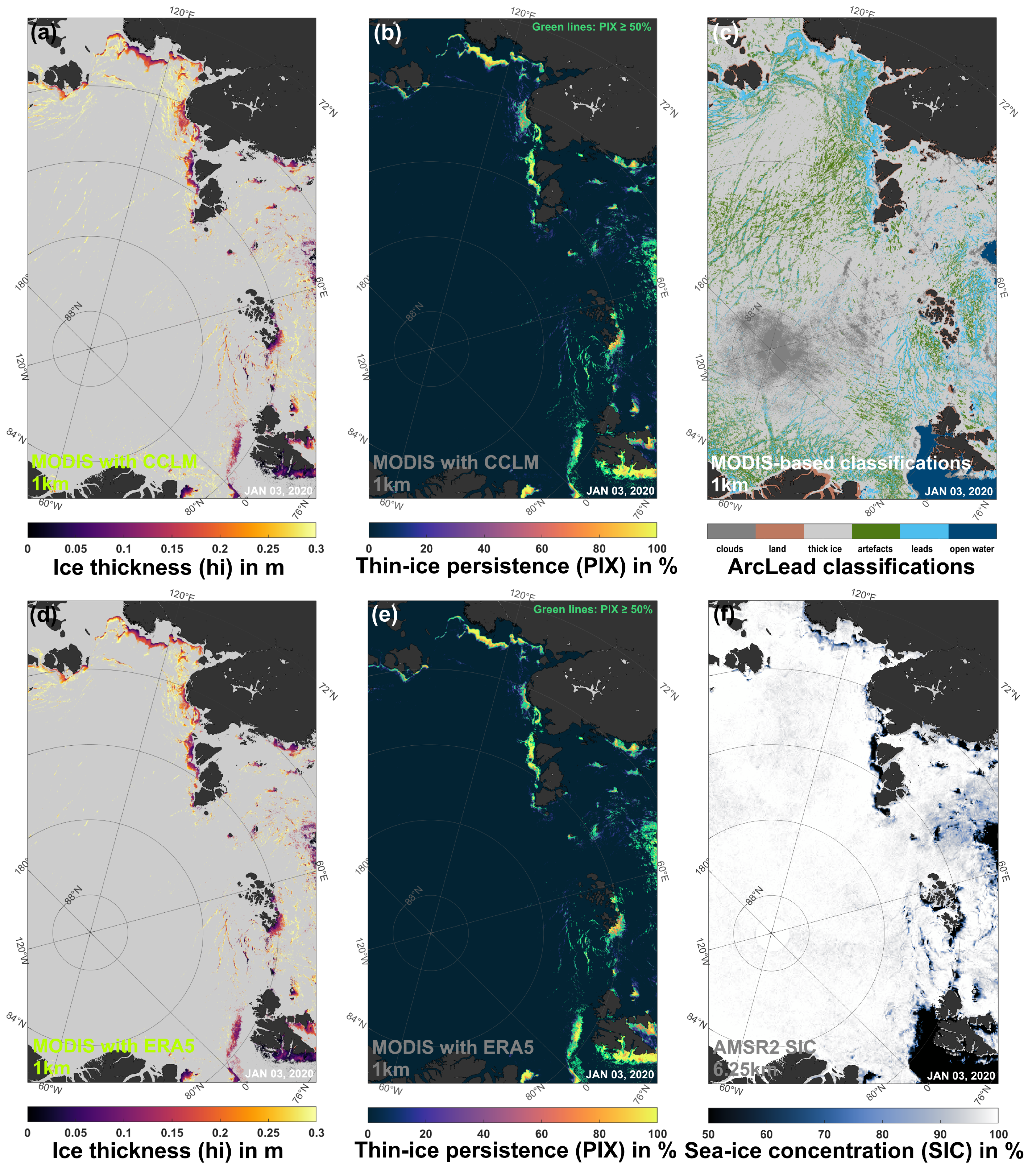
Overview of different data products on 3 January 2020. Thin-ice thicknesses (in m) in the areas of the Laptev Sea and Transpolar Drift ((a) using CCLM data, (d) using ERA5 data) are shown together with their respective daily thin-ice persistence (PIX) value in % ((b) using CCLM data, (e) using ERA5 data). Panel (c) presents daily ArcLead classifications [4], with color labels depicted below the map. Passive microwave sea-ice concentrations (SIC, in %; [21]) from AMSR2 are complementary illustrated in Panel (f).
Figure 3.
Overview of different data products on 3 January 2020. Thin-ice thicknesses (in m) in the areas of the Laptev Sea and Transpolar Drift ((a) using CCLM data, (d) using ERA5 data) are shown together with their respective daily thin-ice persistence (PIX) value in % ((b) using CCLM data, (e) using ERA5 data). Panel (c) presents daily ArcLead classifications [4], with color labels depicted below the map. Passive microwave sea-ice concentrations (SIC, in %; [21]) from AMSR2 are complementary illustrated in Panel (f).

Figure 4.
Scatterplots of the difference in surface temperatures (dTs) versus the difference in 2 m temperatures (dT2m) from CCLM simulations at 15 km grid resolution (both for January 2020). All values are given in °C. Panel (a) features all grid points with a surface temperature < −1.7 °C, while in panel (b) a 70% SIC polynya criteria is applied. Linear regression lines are drawn in red, and the 1:1 line in blue for reference.

Figure 5.
Case study in the Laptev Sea subset-region, illustrating the effect of the dew-point correction within MATA. (a) ERA5 with correction, (b) ERA5 without correction, (c) resulting difference in . All displayed values in g/kg for 2 January 2020, 0425UTC. Black contours indicate areas with ice thicknesses up to 0.2 m. Note the data-gaps (in grey) resulting from the omission of temperature values with no corresponding MODIS IST.

Figure 6.
Case study in the Laptev Sea subset-region, showing the total effect of MATA on the 2 m temperature distribution. Panels (a,d) show from ERA5 and CCLM, respectively, with MATA and the correction applied. (b,e) show the respective distributions without an application of MATA, while (c,f) feature the resulting differences in . All displayed values in K for 2 January 2020, 0425UTC. Black contours indicate areas with ice thicknesses up to 0.2 m. Note the data-gaps (in grey) resulting from the omission of temperature values with no corresponding MODIS IST. Points A (74.22°N, 123.09°E) and B (75.16°N, 124.48°E) mark the transect-line for the extraction of various profiles (Figure 7).

Figure 7.
Various profiles (A to B; cf. Figure 6) for sea-ice and atmospheric variables for the case study in the Laptev Sea on 02 January 2020, 04:25UTC (CCLM vs. ERA5; with/without MATA). (a) Calculated thin ice thicknesses (, in m), (b) sea-ice production scaled to one hour (SIP, in cm/h), (c) 2 m air temperatures and MODIS IST (all in K), (d) specific humidity (, in g/kg), and (e) sensible heat flux (in W/m2). Gaps in all panels result from clouds or otherwise missing IST data.

Figure 8.
Spatial distributions of thin-ice thicknesses (TIT, in m) in the Laptev Sea, presented as persistence-lead-filtered (PLF) daily composites for 2 January 2020. Both CCLM and ERA5 are compared, with (panels (a,c)) and without (panels (b,d)) the application of MATA. Green contours mark areas with ice thicknesses below or equal to 0.2 m.

Figure 9.
Laptev Sea: (a) Daily polynya area (POLA, in km2), (b) accumulated sea-ice production (SIP, in km3) and (c) average thin-ice thickness (, in cm) between December 2019 and April 2020. Both CCLM and ERA5 are compared (based on PLF daily composites), with and without the application of MATA.
Figure 9.
Laptev Sea: (a) Daily polynya area (POLA, in km2), (b) accumulated sea-ice production (SIP, in km3) and (c) average thin-ice thickness (, in cm) between December 2019 and April 2020. Both CCLM and ERA5 are compared (based on PLF daily composites), with and without the application of MATA.

Figure 10.
Laptev Sea: Daily averages of (a) 2 m temperatures (in K), (b) 10m wind speeds (in m/s) and (c) the sensible heat flux (in W/m2) between December 2019 and April 2020. Both CCLM and ERA5 are compared (based on PLF daily composites), with and without the application of MATA.
Figure 10.
Laptev Sea: Daily averages of (a) 2 m temperatures (in K), (b) 10m wind speeds (in m/s) and (c) the sensible heat flux (in W/m2) between December 2019 and April 2020. Both CCLM and ERA5 are compared (based on PLF daily composites), with and without the application of MATA.

Figure 11.
Spatial overview of accumulated sea-ice production (SIP, in m/winter for all TIT ≤ 0.2 m) in the Arctic for December 2019 to April 2020, based on MODIS data at 1km spatial resolution and atmospheric data from CCLM ((a) MATA, (b) no MATA) and ERA5 ((c) MATA, (d) no MATA). Panels (e,f) show the difference in SIP between CCLM and ERA5 for the MATA and no MATA versions, respectively. In contrast to colored areas, pixels in light grey indicate zero SIP as well as masked ocean areas of the northern Atlantic and Pacific seas.


Table 1.
Overview of atmospheric data sets.
| CCLM | ECMWF ERA5 | |
|---|---|---|
| Reference | Modified from [22,23] | [14] |
| Grid Resolution | 5 km or 15 km | 31 km |
| Model type | Regional climate model (Arctic) | Global reanalysis |
| Sea-ice reference | AMSR-E, AMSR2 SIC | SSM/I, SSMIS SIC |
| (U Bremen; ASI-v5.4 [21]), | (OSI-SAF; OSI-401/409 [27] as | |
| MODIS SIC [4] | part of OSTIA [28]) | |
| Utilized variables | , , , , | , , , , |
| , | , , |
Table 2.
Overview of CCLM simulation runs and determined regression parameters performed during MATA development.
Table 2.
Overview of CCLM simulation runs and determined regression parameters performed during MATA development.
| Domain | km | Month | SIC ≤ 0.7 & < −1.7 °C | SIC ≤ 0.7 & < −1.7 °C | <−1.7 °C | |||
|---|---|---|---|---|---|---|---|---|
| (Surrounding Six Pixels) | ||||||||
| slope | r2 | slope | r2 | slope | r2 | |||
| Arctic | 15 | January 2020 | 0.45 | 0.94 | 0.39 | 0.89 | 0.53 | 0.83 |
| Arctic | 15 | April 2020 | 0.48 | 0.93 | 0.49 | 0.95 | 0.61 | 0.89 |
| Arctic | 15 | March 2014 | 0.45 | 0.94 | 0.45 | 0.94 | 0.58 | 0.84 |
| Laptev Sea | 5 | January 2020 | 0.40 | 0.93 | 0.38 | 0.94 | 0.57 | 0.82 |
| Laptev Sea | 5 | April 2020 | 0.41 | 0.90 | 0.39 | 0.91 | 0.65 | 0.86 |
| Barents Sea | 5 | March 2014 | 0.43 | 0.85 | 0.42 | 0.84 | 0.66 | 0.83 |
Table 3.
Accumulated sea-ice production (SIP, in km3) in Arctic polynyas in 2019/2020 (December to March (DJFM)/April (DJFMA)), compared to the long-term average from 2002/2003 to 2017/2018 from Preußer et al. (2019) [2]. Percentages in brackets indicate the relative change that results from applying MATA, both for ERA5 and CCLM, respectively.
| ERA5 | CCLM | ERA Interim [2] | |||||
|---|---|---|---|---|---|---|---|
| no MATA | MATA | MATA | no MATA | MATA | MATA | 2002/2003 to | |
| 2019/2020 | 2019/2020 | 2019/2020 | 2019/2020 | 2019/2020 | 2019/2020 | 2017/2018 | |
| (DJFMA) | (DJFMA) | (DJFM) | (DJFMA) | (DJFMA) | (DJFM) | (DJFM) | |
| Canadian Arctic | 107 | 48 (−55%) | 34 | 224 | 64 (−71%) | 47 | 129 ± 36 |
| Chukchi Sea | 134 | 106 (−21%) | 106 | 289 | 124 (−57%) | 121 | 85 ± 34 |
| East Siberian Sea | 115 | 54 (−53%) | 46 | 322 | 80 (−75%) | 67 | 51 ± 25 |
| Franz-Josef-Land | 81 | 57 (−30%) | 57 | 139 | 64 (−54%) | 63 | 86 ± 33 |
| Kara Sea | 187 | 110 (−41%) | 96 | 322 | 130 (−60%) | 112 | 181 ± 94 |
| Laptev Sea | 132 | 68 (−48%) | 63 | 261 | 82 (−69%) | 75 | 70 ± 28 |
| Northeast Water | 20 | 11 (−45%) | 11 | 51 | 18 (−65%) | 17 | 16 ± 6 |
| North Water | 126 | 74 (−41%) | 69 | 297 | 113 (−62%) | 105 | 196 ± 58 |
| Storfjorden | 21 | 13 (−38%) | 13 | 22 | 17 (−23%) | 16 | 18 ± 6 |
| Severnaya Zemlya | 13 | 8 (−38%) | 8 | 34 | 10 (−71%) | 10 | 18 ± 10 |
Publisher’s Note: MDPI stays neutral with regard to jurisdictional claims in published maps and institutional affiliations. |
© 2022 by the authors. Licensee MDPI, Basel, Switzerland. This article is an open access article distributed under the terms and conditions of the Creative Commons Attribution (CC BY) license (https://creativecommons.org/licenses/by/4.0/).
Share and Cite
MDPI and ACS Style
Preußer, A.; Heinemann, G.; Schefczyk, L.; Willmes, S. A Model-Based Temperature Adjustment Scheme for Wintertime Sea-Ice Production Retrievals from MODIS. Remote Sens. 2022, 14, 2036. https://0-doi-org.brum.beds.ac.uk/10.3390/rs14092036
AMA Style
Preußer A, Heinemann G, Schefczyk L, Willmes S. A Model-Based Temperature Adjustment Scheme for Wintertime Sea-Ice Production Retrievals from MODIS. Remote Sensing. 2022; 14(9):2036. https://0-doi-org.brum.beds.ac.uk/10.3390/rs14092036
Chicago/Turabian StylePreußer, Andreas, Günther Heinemann, Lukas Schefczyk, and Sascha Willmes. 2022. "A Model-Based Temperature Adjustment Scheme for Wintertime Sea-Ice Production Retrievals from MODIS" Remote Sensing 14, no. 9: 2036. https://0-doi-org.brum.beds.ac.uk/10.3390/rs14092036
Note that from the first issue of 2016, this journal uses article numbers instead of page numbers. See further details here.