
Assessment of Estimated Phycocyanin and Chlorophyll-a Concentration from PRISMA and OLCI in Brazilian Inland Waters: A Comparison between Semi-Analytical and Machine Learning Algorithms
 , , , , and
Abstract
:1. Introduction
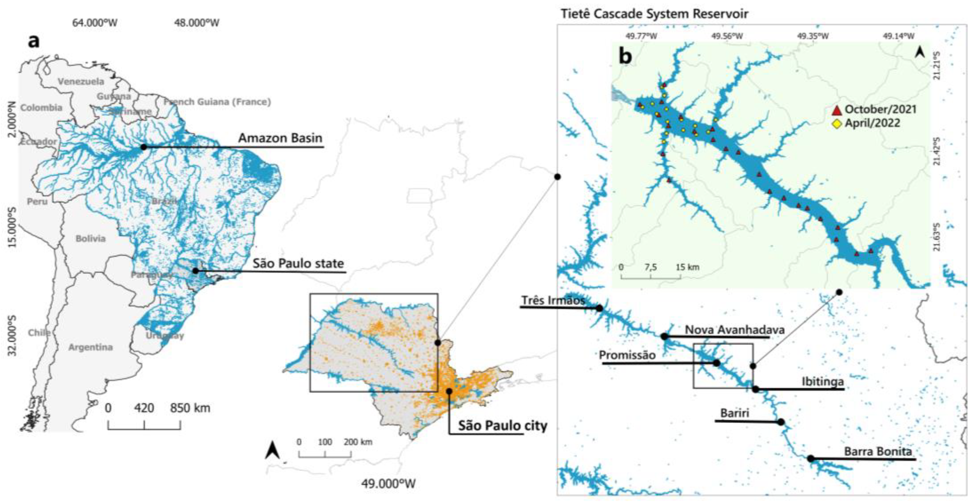
2. Study Area
3. Dataset
3.1. Field Measurements
Laboratory Analysis
3.2. Satellite Imagery Data
3.2.1. PRISMA
3.2.2. OLCI
3.2.3. Available Dataset
4. Methods
4.1. Satellite Imagery Processing
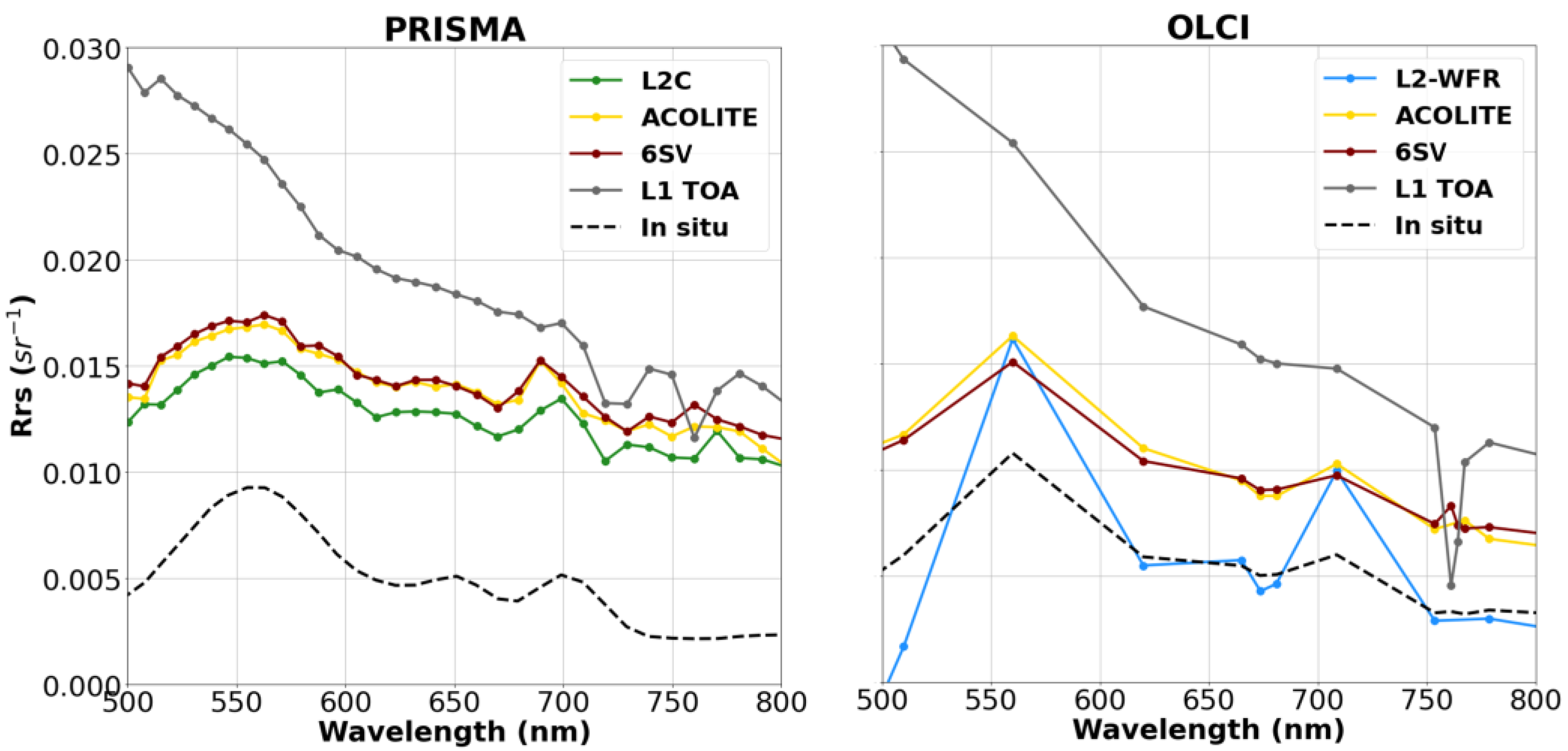
4.1.1. Atmospheric Correction
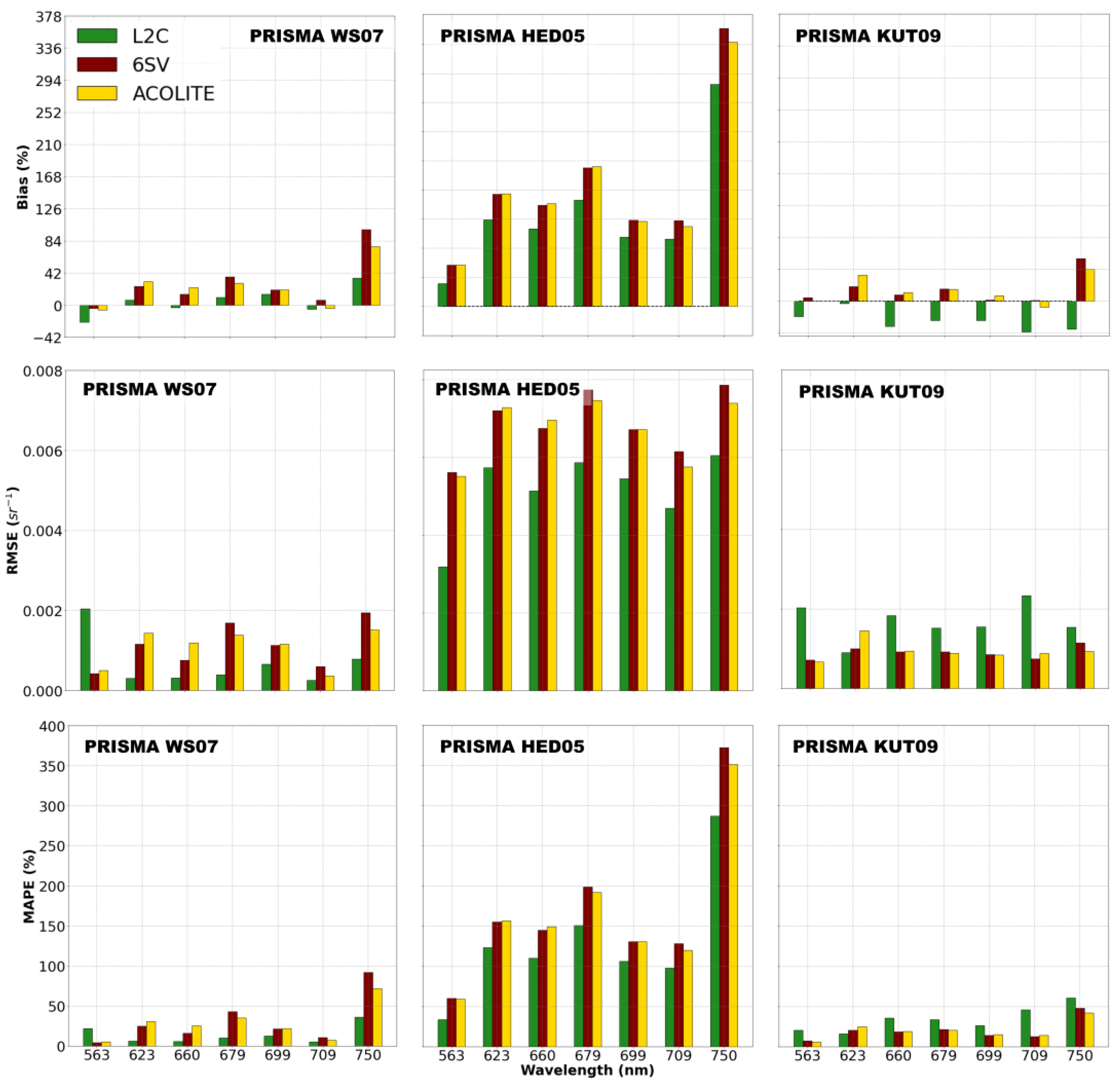
- Standard PRISMA L2C processor: The L2 standard AC processor is based on MODTRAN v6.0, using a multi-dimensional Look-Up-Table (LUT) approach [27]. This method uses the hyperspectral bands to derive atmospheric parameters (e.g., water vapor and Aerosol Optical Depth (AOD)). The water vapor is retrieved pixel-by-pixel using the water’s absorption features at NIR bands. The retrieval of PRISMA AOD is based on the Dense Dark Vegetation (DDV) algorithm approach [49], exploiting the correlation between reflectance in the SWIR region, blue, and red bands. An extended description of the algorithms used to generate PRISMA products is available in [50].
- OLCI L2-WFR: The baseline AC algorithm (BAC) used in OLCI L2 products is a combination of NIR-based black-pixel assumption with bright-pixel AC (BPAC). BPAC corrects the contribution of sediments when the water-leaving reflectance is no longer negligible in NIR bands, as is the case for coastal and inland turbid waters. It consists of decoupling the oceanic and atmospheric components of the NIR bands in order to apply the standard AC scheme [51].
- 6SV (for both PRISMA and OLCI): Second Simulation of a Satellite Signal in the Solar Spectrum (6SV) is an advanced radiative transfer code designed to simulate a specific condition of the atmosphere based on advance knowledge of atmospheric and illumination conditions and the sensor used. The algorithm takes as input the necessary parameters to apply the radiative transfer equation for estimating the surface reflectance [32]. For the validation of PRISMA L1 and OLCI L1 products, 6SV was applied using the Py6S Python programming language interface [52]. The aerosol and atmospheric profiles were set as Continental and Tropical, respectively. The AOD (550) value and the geometry parameters were obtained from PRISMA metadata. The correction was made for each PRISMA and OLCI band using their respective SRFs.
- ACOLITE (for both PRISMA and OLCI): The current version of ACOLITE (20220222.0) applies a dark spectrum fitting (DSF) scheme as the default setting to estimate the AOD and, hence, atmospheric path reflectance, transmittances, and spherical albedo [33]. The DSF assumes: (i) a homogeneous atmosphere over a certain extent of an image, and (ii) that there are pixels within this subscene that contain near-zero water-leaving radiances in one band. A pre-generated LUT is utilized to find the dominant aerosol condition. Despite being primarily designed for processing multispectral images, ACOLITE is now adapted to support processing of PRISMA data where the L1 and L2C data products are required as inputs. The ACOLITE/DSF processing (version 20220222.0) is available in a GitHub code repository and in binary releases (https://github.com/acolite/acolite, accessed on 25 February 2023).
4.1.2. Glint Correction
- The Wang and Shi [53] (WS07) method assume that the reflectance values of SWIR bands come from the specular reflection in the water’s surface (sun and sky glint), as the signal from this spectral region is considered negligible in natural inland waters [26]. Considering the 173 SWIR channels from PRISMA (942–2496 nm), a SWIR-range band centered near 1600 nm [1533.56–1745.93 nm] was considered as the reference band for performing the glint correction. In principle, a band range centered near 2200 nm could also be selected as reference. However, these bands are much noisier than 1600 nm [54]. Therefore, in order to avoid the possible noise propagation to the glint-removed bands in the visible region, the 1600 nm SWIR band was selected as the reference band, where the average was considered and then subtracted from each band in the VNIR spectrum.
- The Hedley et al. [55] (HED05) method assumes negligible water-leaving signal in the NIR part of the spectrum. Relative sun-glint intensity of the image is obtained based on the NIR brightness and the light in the visible band using a set of pixels, which could be homogeneous if not for the presence of glint. Establishing a linear relationship between the NIR band and each visible band allows for the removal of the glint contribution. In case of hyperspectral data there is a need to find the regression algorithm for each spectral band. The HED05 method was used in a deglint processor implemented in the Sen2Coral toolbox available in the SNAP software (https://sen2coral.argans.co.uk/, accessed on 25 February 2023). Bands between 833–972 nm were considered as glint reference.
- Kutser et al. [56] (KUT09) proposed an alternative glint removal procedure for hyperspectral imagery when SWIR data is not available. The method is based on the assumption that there is no spectral feature in the at 760 nm if it does not contain glint. Furthermore, it considers that the depth of an oxygen absorption feature at 760 nm (called D) is proportional to the amount of glint in this pixel. The model assumes that pixels with D values close to zero do not contain glint and pixels with the highest D value contain mainly glint. By subtracting the pixel spectrum in which D is close to zero from the spectrum with the highest D, the glint spectrum is obtained. In order to avoid land pixels or adjacency pixels, before the application of the model, a water mask must be applied.
4.1.3. Performance Assessment (Radiometry)
4.2. Phycocyanin and Chlorophyll-a Modeling
4.2.1. Nested Band Semi-Analytical Algorithm
4.2.2. Machine Learning Models
4.2.3. Performance Indicators (Algorithms)
5. Results and Discussion
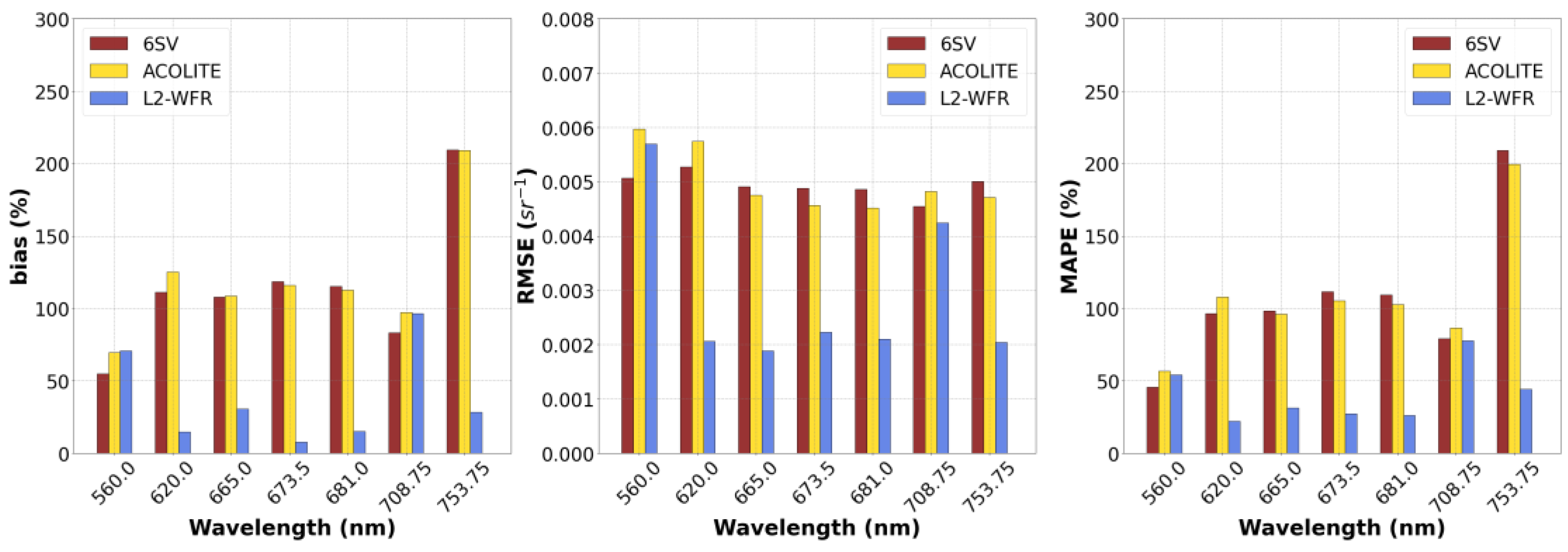
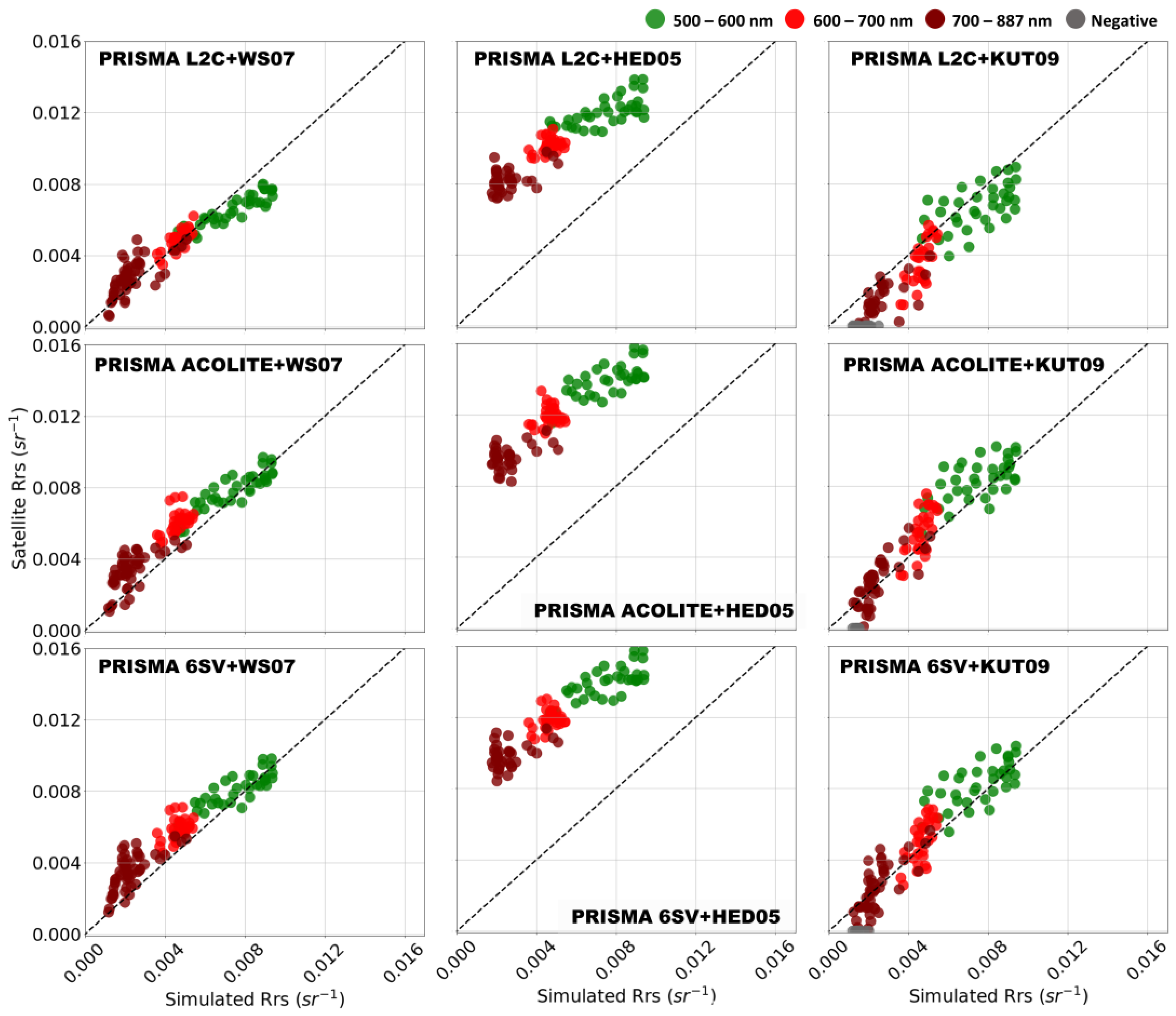
5.1. Atmospheric and Glint Correction
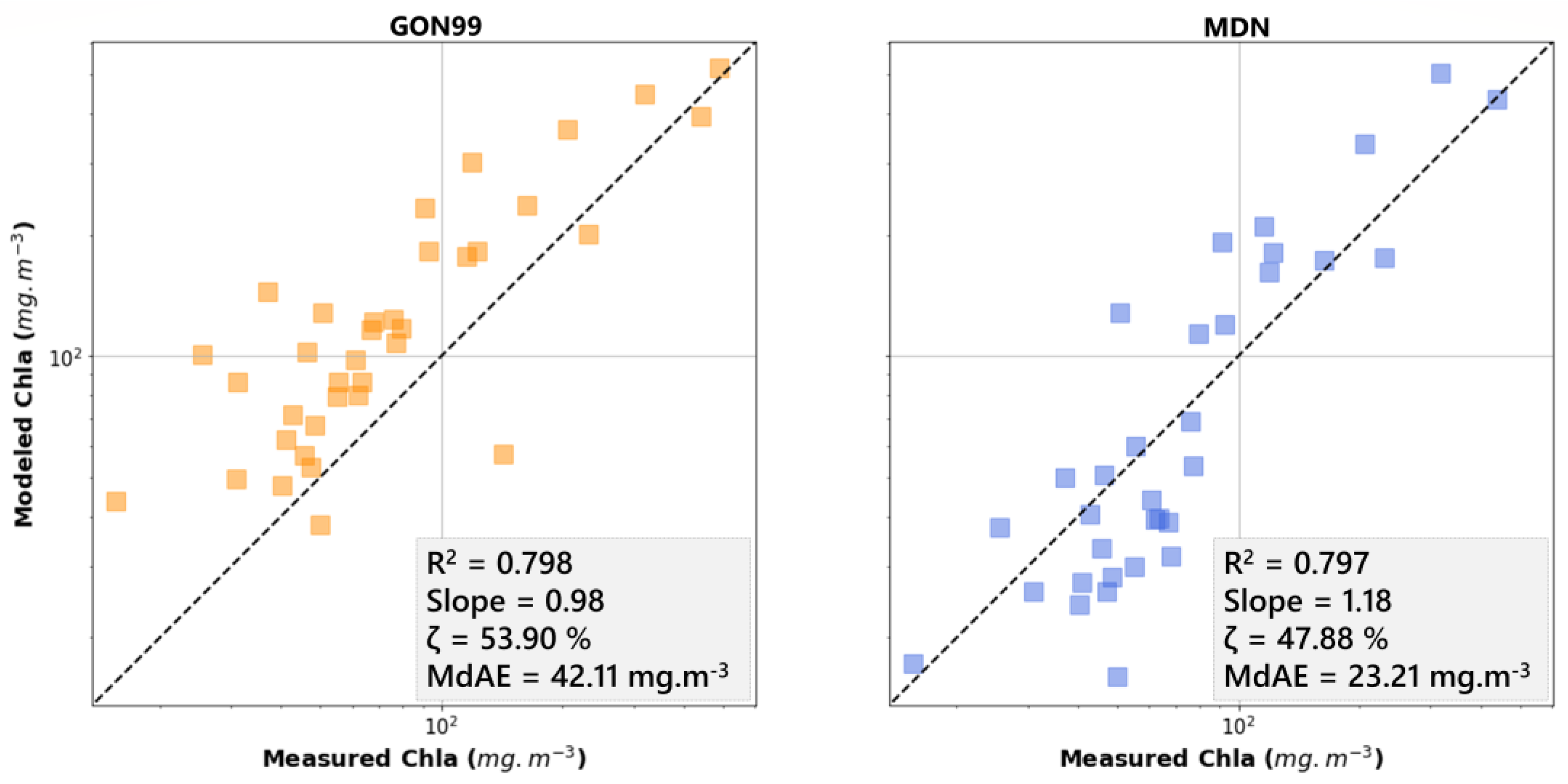
5.2. Phycocyanin and Chlorophyll-a Algorithm Performance
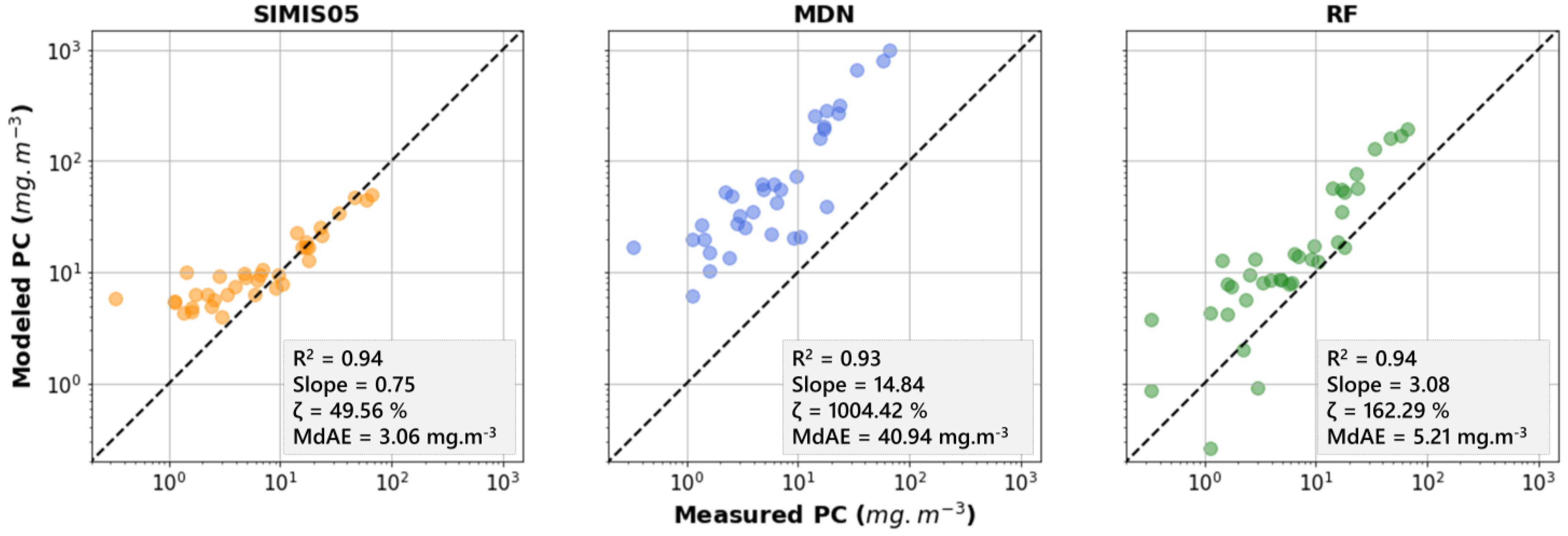
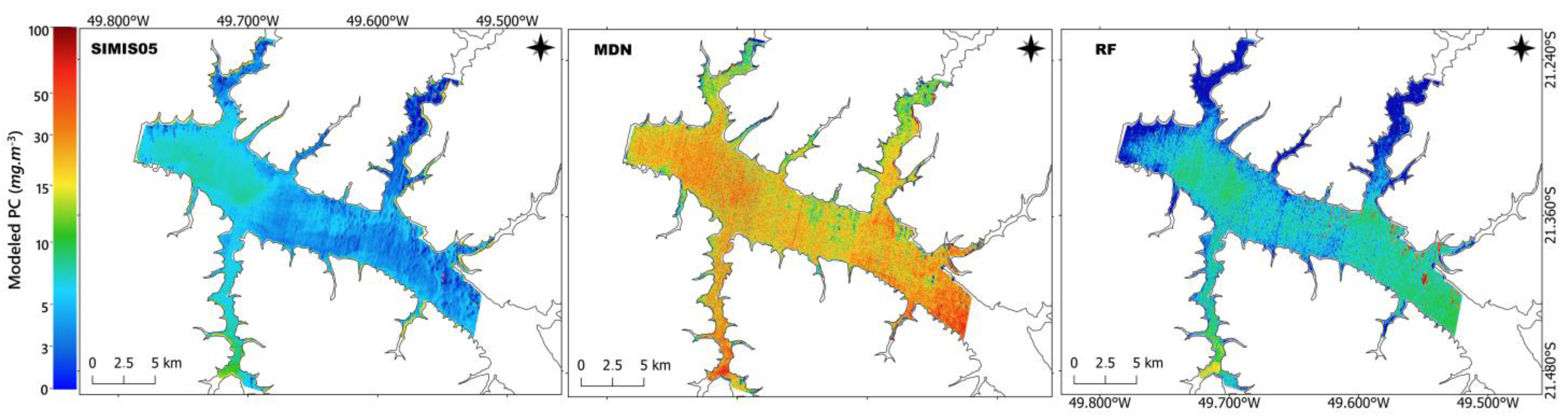
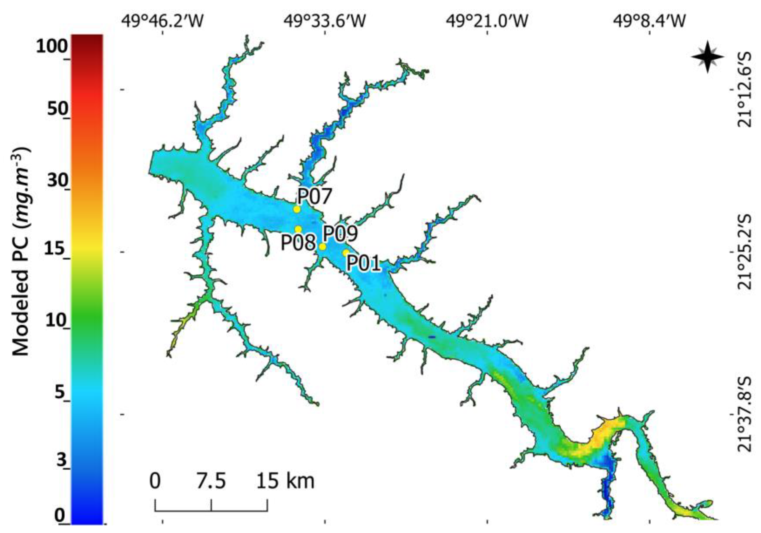
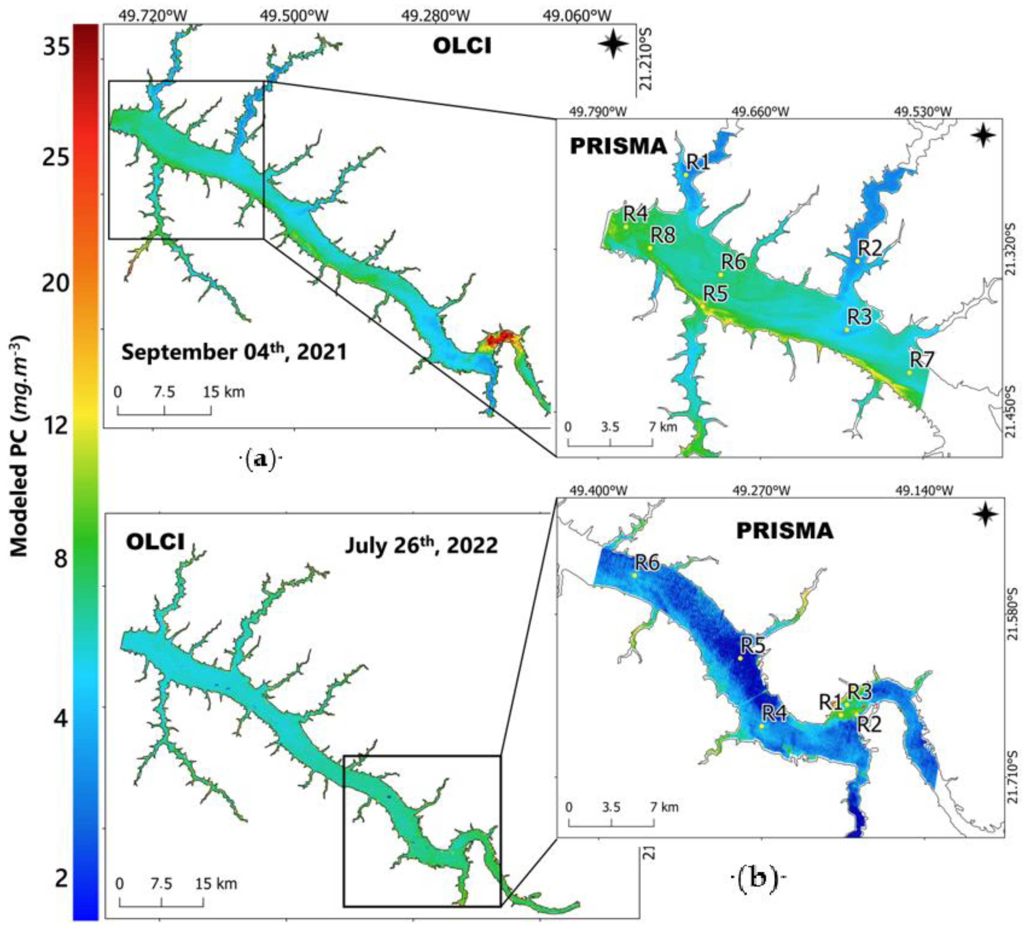
5.3. Mapping PC: Model Assessment on Satellite Observations
6. Conclusions
Author Contributions
Funding
Data Availability Statement
Acknowledgments
Conflicts of Interest
References
- Miola, A.; Schiltz, F. Measuring sustainable development goals performance: How to monitor policy action in the 2030 Agenda implementation? Ecol. Econ. 2019, 164, 106379. [Google Scholar] [CrossRef] [PubMed]
- Azevedo, S.M.F.O.; Vasconcelos, V.M. Toxinas de cianobactérias: Causas e Consequências para a saúde pública. In Ecotoxicologia Aquática: Príncipios e Aplicações, 1st ed.; Zagatto, P.A., Bertoletti, E., Eds.; Rima: Rio de Janeiro, Brazil, 2006; pp. 433–452. [Google Scholar]
- Giuliani, G.; Nativi, S.; Obregon, A.; Beniston, M.; Lehmann, A. Spatially enabling the Global Framework for Climate Services: Reviewing geospatial solutions to efficiently share and integrate climate data & information. Clim. Serv. 2017, 8, 44–58. [Google Scholar] [CrossRef]
- Lehmann, A.; Chaplin-Kramer, R.; Lacayo, M.; Giuliani, G.; Thau, D.; Koy, K.; Goldberg, G.; Sharp, R., Jr. Lifting the Information Barriers to Address Sustainability Challenges with Data from Physical Geography and Earth Observation. Sustainability 2017, 9, 858. [Google Scholar] [CrossRef] [Green Version]
- Shi, K.; Zhang, Y.; Qin, B.; Zhou, B. Remote sensing of cyanobacterial blooms in inland waters: Present knowledge and future challenges. Sci. Bull. 2019, 64, 1540–1556. [Google Scholar] [CrossRef] [Green Version]
- Coffer, M.M.; Schaeffer, B.A.; Foreman, K.; Porteous, A.; Loftin, K.A.; Stumpf, R.P.; Darling, J.A. Assessing cyanobacterial frequency and abundance at surface waters near drinking water intakes across the United States. Water Res. 2021, 201, 117377. [Google Scholar] [CrossRef]
- Schaeffer, B.A.; Urquhart, E.; Coffer, M.; Salls, W.; Stumpf, R.P.; Loftin, K.A.; Werdell, P.J. Satellites quantify the spatial extent of cyanobacterial blooms across the United States at multiple scales. Ecol. Indic. 2022, 140, 108990. [Google Scholar] [CrossRef]
- Jang, M.T.G.; Alcântara, E.; Rodrigues, T.; Park, E.; Ogashawara, I.; Marengo, J.A. Increased chlorophyll-a concentration in Barra Bonita reservoir during extreme drought periods. Sci. Total Environ. 2022, 843, 157106. [Google Scholar] [CrossRef]
- Ogashawara, I. Determination of phycocyanin from space-A bibliometric analysis. Remote Sens. 2020, 12, 567. [Google Scholar] [CrossRef] [Green Version]
- Pahlevan, N.; Smith, B.; Schalles, J.; Binding, C.; Cao, Z.; Ma, R.; Stumpf, R. Seamless retrievals of chlorophyll-a from Sentinel-2 (MSI) and Sentinel-3 (OLCI) in inland and coastal waters: A machine-learning approach. Remote Sens. Environ. 2020, 240, 111604. [Google Scholar] [CrossRef]
- Dierssen, H.M. Realizing the potential of hyperspectral remote sensing in coastal and inland waters. In Proceedings of the IEEE International Geoscience and Remote Sensing Symposium IGARSS, Brussels, Belgium, 11–16 July 2021. [Google Scholar] [CrossRef]
- Karger-Muller, F.E.; Hestir, E.; Ade, C.; Turpie, K.; Roberts, D.A.; Siegel, D.; Miller, R.J.; Humm, D.; Izenberg, N.; Keller, M.; et al. Satellite sensor requirements for monitoring essential biodiversity variables of coastal ecosystems. Ecol. Appl. 2018, 28, 749–760. [Google Scholar] [CrossRef] [Green Version]
- Ahn, C.Y.; Joung, S.H.; Yoon, S.K.; Oh, H.M. Alternative alert system for cyanobacterial bloom, using phycocyanin as level determinant. J. Microbiol. 2007, 45, 98–104. [Google Scholar] [PubMed]
- Augusto-Silva, P.B.; Ogashawara, I.; Barbosa, C.C.; De Carvalho, L.A.S.; Jorge, D.S.F.; Fornari, C.I.; SteCH, J. Analysis of MERIS Reflectance Algorithms for Estimating Chlorophyll-a Concentration in a Brazilian Reservoir. Remote Sens. 2014, 6, 11689–11707. [Google Scholar] [CrossRef] [Green Version]
- Watanabe, F.S.Y.; Alcântara, E.; Rodrigues, T.W.P.; Imai, N.N.; Barbosa, C.C.F.; Rotta, L.H.S. Estimation of chlorophyll-a concentration and the trophic state of the Barra Bonita Hydroelectric Reservoir using OLI/Landsat-8 images. Int. J. Environ. Res. Public Health 2015, 12, 10391–10417. [Google Scholar] [CrossRef] [PubMed] [Green Version]
- Cairo, C.; Barbosa, C.C.F.; Lobo, F.L.; Novo, E.M.L.M. Hybrid Chlorophyll-a Algorithm for Assessing Trophic States of a Tropical Brazilian Reservoir Based on MSI/Sentinel-2 Data. Remote Sens. 2020, 12, 40. [Google Scholar] [CrossRef] [Green Version]
- Dekker, A.G. Detection of Optical Water Quality Parameters for Eutrophic Waters by High Resolution Remote Sensing. Ph.D. Thesis, Doctorate in Research and graduation internal—Vrije University, Amsterdam, The Netherlands, 1993. [Google Scholar]
- Schalles, J.F.; Yacobi, Y.Z. Remote detection and seasonal patterns of phycocyanin, carotenoid and chlorophyll pigments in eutrophic waters. Arch. Fur Hydrobiol. 2000, 55, 153–168. [Google Scholar] [CrossRef]
- Kutser, T. Quantitative detection of chlorophyll in cyanobacterial blooms by satellite remote sensing. Limnol. Oceanogr. 2004, 49, 2179–2189. [Google Scholar] [CrossRef]
- Simis, S.G.H.; Ruiz-Verdu, A.; Dominguez-Gomez, J.A.; Pena-Martinez, R.; Peters, S.W.M.; Gons, H.J. Influence of phytoplankton pigment composition on remote sensing of cyanobacterial biomass. Remote Sens. Environ. 2007, 106, 414–427. [Google Scholar] [CrossRef]
- Li, L.; Li, L.; Song, K. Remote sensing of freshwater cyanobacteria: An extended IOP Inversion Model of Inland Waters (IIMIW) for partitioning absorption coefficient and estimating phycocyanin. Remote Sens. Environ. 2015, 157, 9–23. [Google Scholar] [CrossRef]
- Simis, S.G.H.; Peters, S.W.M.; Gons, H.J. Remote sensing of the cyanobacterial pigment phycocyanin in turbid inland water. Limnol. Oceanogr. 2005, 50, 237–245. [Google Scholar] [CrossRef]
- Ruiz-Verdú, A.; Simis, S.G.H.; de Hoyos, C.; Gons, H.J.; Peña-Martínez, R. An evaluation of algorithms for the remote sensing of cyanobacterial biomass. Remote Sens. Environ. 2008, 112, 3996–4008. [Google Scholar] [CrossRef]
- Yan, Y.; Bao, Z.; Shao, J. Phycocyanin concentration retrieval in inland waters: A comparative review of the remote sensing techniques and algorithms. J. Great Lakes Res. 2018, 44, 748–755. [Google Scholar] [CrossRef]
- Riddick, C.A.L.; Hunter, P.D.; Domínguez-Gómez, J.A.; Martinez-Vicente, V.; Présing, M.; Horváth, H.; Kovács, A.W.; Vörös, L.; Zsigmond, E.; Tyler, A.N. Optimal Cyanobacterial Pigment Retrieval from Ocean Colour Sensors in a Highly Turbid, Optically Complex Lake. Remote Sens. 2019, 11, 1613. [Google Scholar] [CrossRef] [Green Version]
- O’shea, R.E.; Pahlevan, N.; Smith, B.; Bresciani, M.; Egerton, T.; Giardino, C.; Li, L.; Moore, T.; Ruiz-Verdu, A.; Ruberg, S.; et al. Advancing cyanobacteria biomass estimation from hyperspectral observations: Demonstrations with HICO and PRISMA imagery. Remote Sens. Environ. 2021, 266, 112693. [Google Scholar] [CrossRef]
- Braga, F.; Fabbretto, A.; Vanhellemont, Q.; Bresciani, M.; Giardino, C.; Scarpa, G.M.; Manfè, G.; Concha, J.A.; Brando, V.E. Assessment of PRISMA water reflectance using autonomous hyperspectral radiometry. ISPRS J. Photogramm. Remote Sens. 2022, 192, 99–114. [Google Scholar] [CrossRef]
- Niroumand-Jadidi, M.; Bovolo, F.; Bruzzone, L. Water quality retrieval from PRISMA Hyperspectral images: First experience in a turbid lake and comparison with Sentinel-2. Remote Sens. 2020, 12, 3984. [Google Scholar] [CrossRef]
- Bresciani, M.; Giardino, C.; Fabbretto, A.; Pellegrino, A.; Mangano, S.; Free, G.; Pinardi, M. Application of new hyperspectral sesors in the remote sensing of aquatic ecosystem health: Exploiting PRISMA and DESIS for four Italian lakes. Resources 2022, 11, 8. [Google Scholar] [CrossRef]
- Borfecchia, F.; Micheli, C.; De Cecco, L.; Sannino, G.; Struglia, M.V.; Di Sarra, A.G.; Mattiazzo, G. Satellite multi/hyper spectral HR sensors for mapping the Posidonia oceanica in south mediterranean islands. Sustainability 2021, 13, 13715. [Google Scholar] [CrossRef]
- Cogliati, S.; Sarti, F.; Chiarantini, L.; Cosi, M.; Lorusso, R.; Lopinto, E.; Colombo, R. The PRISMA imaging spectroscopy mission: Overview and first performance analysis. Remote Sens. Environ. 2021, 262, 112499. [Google Scholar] [CrossRef]
- Vanhellemont, Q. Adaptation of the dark spectrum fitting atmospheric correction for aquatic applications of the Landsat and Sentinel-2 archives. Remote Sens. Environ. 2019, 225, 175–192. [Google Scholar] [CrossRef]
- Vermote, E.; Tanre, D.; Deuze, J.L.; Herman, M.; Morcrette, J.J.; Kotchenova, S.Y. Second simulation of a satellite signal in the solar sprectrum, 6S: An overview. IEEE Trans. Geosci. Remote Sens. 1997, 35, 675–686. [Google Scholar] [CrossRef] [Green Version]
- Barbosa, C.C.F.; Novo, E.M.L.M.; Martins, V.S. Introdução ao Sensoriamento Remoto de Sistemas Aquáticos: Princípios e Aplicações, 1st ed.; INPE: São José dos Campos, Brazil, 2019; 178p, ISBN 978-85-17-0009-9. [Google Scholar]
- Bernardo, N.; Alcântara, E.; Watanabe, F.; Rodrigues, T.; Carmo, A.; Gomes, A.; Andrade, C. Glint removal assessment to estimate the remote sensing reflectance in inland waters with widely differing optical properties. Remote Sens. 2018, 10, 1655. [Google Scholar] [CrossRef] [Green Version]
- Mobley, C.D. Estimation of the remote-sensing reflectance from above-surface measurements. Appl. Opt. 1999, 38, 7442–7455. [Google Scholar] [CrossRef] [PubMed]
- Mueller, J.L.; Austin, R.W. SeaWiFS Technical Report Series. NASA Tech. Memo. 1995, 25. [Google Scholar]
- Kutser, T.; Vahtmae, E.; Paavel, B.; Kauer, T. Removing glint effects from field radiometry data measured in optically complex coastal and inland waters. Remote Sens. Environ. 2013, 113, 85–89. [Google Scholar] [CrossRef]
- Pelloquin, C.; Nieke, J. Sentinel-3 OLCI and SLSTR simulated spectral response function. Tech. Note 2012, 1, S3-TN-ESA-PL-316. [Google Scholar] [CrossRef]
- Tassan, S.; Ferrari, G.M. A sensitivity analysis of the ‘Transmittance-Reflectance’ method for measuring light absorption by aquatic particles. J. Plankton Res. 2002, 24, 757–774. [Google Scholar] [CrossRef]
- Roesler, C.S. Theoretical and experimental approaches to improve the accuracy of particulate absorption coefficients derived from the quantitative filter technique. Limnol. Oceanogr. 2003, 43, 1649–1660. [Google Scholar] [CrossRef]
- Stramski, D.; Reynolds, R.A.; Kaczmarek, S.; Uitz, J.; Zheng, G. Correction of pathlength amplification in the filter-pad technique for measurements of particulate absorption coefficient in the visible spectral region. Appl. Opt. 2015, 54, 6763–6782. [Google Scholar] [CrossRef] [Green Version]
- APHA. Standard Methods for the Examination of Water and Wastewater, 20th ed.; American Public Health Association: Washington, DC, USA, 1998; 874p. [Google Scholar]
- Sarada, R.; Pillai, M.G.; Ravishankar, G.A. Phycocyanin from Spirulina sp: Influence of processing of biomass on phycocyanin yield, analysis of efficacy of extraction methods and stability studies on phycocyanin. Process Biochem. 1999, 34, 795–801. [Google Scholar] [CrossRef]
- Horváth, H.; Kovács, A.W.; Riddick, C.; Présing, M. Extraction methods for phycocyanin determination in freshwater filamentous cyanobacteria and their application in a shallow lake. Eur. J. Phycol. 2013, 48, 278–286. [Google Scholar] [CrossRef] [Green Version]
- Bennett, A.; Bogorad, L. Complementary chromatic adaptation in a filamentous blue-green alga. J. Cell Biol. 1973, 58, 419–435. [Google Scholar] [CrossRef] [PubMed]
- Giardino, C.; Bresciani, M.; Braga, F.; Fabbretto, A.; Ghirardi, N.; Pepe, M.; Gianinetto, M.; Colombo, R.; Cogliati, S.; Ghebrehiwot, S.; et al. First evaluation of PRISMA Level 1 data for water applications. Sensors 2020, 20, 4553. [Google Scholar] [CrossRef] [PubMed]
- ESA. Sentinel-Online: Product Types Information. Available online: https://sentinels.copernicus.eu/web/sentinel/user-guides/sentinel-3-olci/product-types (accessed on 22 November 2022).
- Ouaidrari, H.; Vermote, E.F. Operational atmospheric correction of Landsat TM data. Remote Sens. Environ. 1999, 70, 4–15. [Google Scholar] [CrossRef]
- ASI. PRISMA Products Specification Document. Issue 2.3. Available online: http://prisma.asi.it/missionselect/docs/PRISMA%20Product%20Specifications_Is2_3.pdf (accessed on 24 October 2022).
- Renosh, P.R.; Doxaran, D.; Keukelaere, L.; GOSSN, J.I. Evaluation of atmospheric correction algorithms for Sentinel-2-MSI and Sentinel-3-OLCI in highly turbide estuarine waters. Remote Sens. 2020, 12, 1285. [Google Scholar] [CrossRef] [Green Version]
- Wilson, R.T. Py6S: A Python interface to the 6S radiative transfer model. Comput. Geosci. 2013, 51, 166–171. [Google Scholar] [CrossRef] [Green Version]
- Wang, M.; Shi, W. The NIR-SWIR combined atmospheric correction approach for MODIS ocean color data processing. Opt. Express 2007, 15, 15722–15733. [Google Scholar] [CrossRef] [Green Version]
- Gao, B.-C.; Montes, M.J.; Davis, C.O.; Goetz, A.F.H. Atmospheric correction algorithms for hyperspectral remote sensing data of land and ocean. Remote Sens. Environ. 2009, 113, 2017–2224. [Google Scholar] [CrossRef]
- Hedley, J.D.; Harbone, A.R.; Mumby, P.J. Simple and robust removal of sun glint for mapping shallow-water benthos. Int. J. Remote Sens. 2005, 26, 2107–2112. [Google Scholar] [CrossRef]
- Kutser, T.; Vahtmae, E.; Praks, J. A sun glint correction method for hyperspectral imagery containing areas with non-negligible water leaving NIR signal. Remote Sens. Environ. 2009, 113, 2267–2274. [Google Scholar] [CrossRef]
- Gordon, H.R.; Brown, O.B.; Jacobs, M.M. Computed relationships between the inherent and apparent optical properties of a flat homogeneous ocean. Appl. Opt. 1975, 14, 417–427. [Google Scholar] [CrossRef]
- Gons, H.J. Optical Teledetection of Chlorophyllain Turbid Inland Waters. Environ. Sci. Technol. 1999, 33, 1127–1132. [Google Scholar] [CrossRef]
- Begliomini, F.N. Cyanobacteria Monitoring on Urban Reservoir Using Hyperspectral Orbital Remote Sensing Data and Machine Learning. Ph.D. Thesis, Master in Remote Sensing—Instituto Nacional de Pesquisas Espaciais (INPE), São José dos Campos, Brazil, 2022. [Google Scholar]
- Hunter, P.D.; Tyler, A.N.; Carvalho, L.; Codd, G.A.; Marberly, S.C. Hyperspectral remote sensing of cyanobacterial pigments as indicators for cell populations and toxins in eutrophic lakes. Remote Sens. Environ. 2010, 114, 2705–2718. [Google Scholar] [CrossRef] [Green Version]
- Mishra, S.; Mishra, D.R. A novel remote sensing algorithm to quantify phycocyanin in cyanobacterial algal blooms. Environ. Res. Lett. 2014, 9, 114003. [Google Scholar] [CrossRef]
- Mishra, S.; Mishra, D.R. Normalized difference chlorophyll index: A novel model for remote estimation of chlorophyll-a concentration in turbid productive waters. Remote Sens. Environ. 2012, 117, 394–406. [Google Scholar] [CrossRef]
- Morley, S.K.; Britto, T.V.; Walling, D.T. Measures of model performance based on the log accuracy ratio. Space Weather 2018, 16, 69–88. [Google Scholar] [CrossRef]
- Kravitz, J.; Matthews, M.; Bernard, S.; Griffith, D. Application of Sentinel 3 OLCI for chl-a retrieval over small inland water targets: Successes and challenges. Remote Sens. Environ. 2020, 237, 111562. [Google Scholar] [CrossRef]
- Moses, J.W.; Steckx, S.; Montes, M.J.; Keukelaere, L.D.; Knaeps, E. Atmospheric Correction for Inland Waters. In Bio-Optical Modeling and Remote Sensing of Inland Waters, 1st ed.; Mishra, D.R., Ogashawara, I., Gitelson, A.A., Eds.; Elsevier: Amsterdam, The Netherlands, 2017; 334p, ISBN 978-0-12-804644-9. [Google Scholar]
- Qiang, Y.; Xindong, W. 10 Challenging problems in data mining research. Int. J. Inf. Technol. Decis. Mak. 2006, 5, 597–604. [Google Scholar]
- Simis, S.G.H.; Kauko, H.M. In vivo mass-specific absorption spectra of phycobilinpigments through selective bleaching. Limnol. Oceanogr. Methods 2012, 10, 214–226. [Google Scholar] [CrossRef]
- Moses, W.J.; Bowles, J.H.; Lucke, R.L.; Corsor, M.R. Impact of signal-to-noise ratio in a hyperspectral sensor on the accuracy of biophysical parameter estimation in case II waters. Opt. Express 2012, 20, 4309–4330. [Google Scholar] [CrossRef]
- Giardino, C.; Brando, V.E.; Gege, P.; Pinnel, N.; Hochberg, E.; Knaeps, E.; Reusen, I.; Doerffer, R.; Bresciani, M.; Braga, F.; et al. Imaging spectrometry of inland and coastal waters: State of the art, achievements and perspectives. Surv. Geophys. 2019, 40, 401–429. [Google Scholar] [CrossRef] [Green Version]
- Dierssen, H.M.; Ackleson, S.G.; Joyce, K.E.; Hestir, E.L.; Castagna, A.; Lavender, S.; Mcmanus, M.A. Living up to the hype of hyperspectral aquatic remote sensing: Science, resources and outlook. Front. Environ. Sci. 2021, 9. [Google Scholar] [CrossRef]
- Harmel, T.; Chami, M.; Tormos, T.; Reynaud, N.; Danis, P.A. Sunglint correction of the Multi-Spectral Instrument (MSI)-SENTINEL-2 imagery over inland and sea waters from SWIR bands. Remote Sens. Environ. 2018, 204, 308–321. [Google Scholar] [CrossRef]


| Min | Max | Mean | Median | Std | ||
|---|---|---|---|---|---|---|
| October/ 2021 | PC | 0.33 | 136.39 | 10.01 | 3.00 | 27.20 |
| Chl-a | 25.44 | 183.47 | 66.51 | 50.04 | 41.00 | |
| PC:Chl-a | 0.008 | 0.74 | 0.095 | 0.073 | 0.14 | |
| April/ 2022 | PC | 1.36 | 65.89 | 26.98 | 18.16 | 19.23 |
| Chl-a | 15.59 | 487.82 | 167.45 | 115.76 | 138.57 | |
| PC:Chl-a | 0.074 | 0.47 | 0.18 | 0.15 | 0.10 |
| Coefficient of Determination | |
| Bias | |
| Root Mean Square Error (RMSE) | |
| Mean Absolute Percentage Error (MAPE) | |
| Spectral Angle (SA) |
| ML Model | Selected Features |
|---|---|
| MDN | MA [17] * (600, 648, 624); BR(650, 625); BR(709, 665); BR(709, 620); BR(700, 600); MA [60] * (725, 615, 600); LH(665, 681, 709); MA [61] * (724, 629, 659); LH(654, 714, 754); LH(665, 709, 754); LH(680, 709, 754); MA [62] * (709, 665); LH(560, 620, 665); LH(665, 673, 681); LH(690, 709, 720); LH(620, 650, 670); LH(640, 650, 660); LH(613, 620, 627). |
| RF | LH(739, 802, 855); NI(563, 555); LH(651, 699, 750); MA [61] * (531, 571, 614) |
| Median Symmetric Accuracy | |
| Median Absolute Error |
| Station | In Situ | PRISMA | OLCI | ||
|---|---|---|---|---|---|
| SIMIS05 | MDN | RF | SIMIS05 | ||
| P07 | 1.12 | 4.69 | 24.46 | 6.23 | 5.17 |
| P08 | 1.12 | 3.89 | 38.68 | 5.09 | 4.93 |
| P09 | 0.33 | 4.12 | 24.16 | 8.65 | 4.57 |
| P01 | 3.33 | 4.07 | 24.97 | 9.05 | 4.69 |
| 4 September 2021 | 26 July 2022 | ||||
|---|---|---|---|---|---|
| ROI | PRISMA | OLCI | ROI | PRISMA | OLCI |
| R01 | 2.42 | 3.32 | R01 | 7.15 | 5.45 |
| R02 | 2.73 | 3.06 | R02 | 25.52 | 7.42 |
| R03 | 3.36 | 3.99 | R03 | 4.20 | 5.56 |
| R04 | 7.98 | 6.92 | R04 | 4.76 | 6.14 |
| R05 | 10.27 | 6.51 | R05 | 0.85 | 6.52 |
| R06 | 6.57 | 5.60 | R06 | 3.52 | 5.91 |
| R07 | 5.64 | 5.21 | - | - | - |
| R08 | 8.17 | 6.64 | - | - | - |
Disclaimer/Publisher’s Note: The statements, opinions and data contained in all publications are solely those of the individual author(s) and contributor(s) and not of MDPI and/or the editor(s). MDPI and/or the editor(s) disclaim responsibility for any injury to people or property resulting from any ideas, methods, instructions or products referred to in the content. |
© 2023 by the authors. Licensee MDPI, Basel, Switzerland. This article is an open access article distributed under the terms and conditions of the Creative Commons Attribution (CC BY) license (https://creativecommons.org/licenses/by/4.0/).
Share and Cite
Lima, T.M.A.d.; Giardino, C.; Bresciani, M.; Barbosa, C.C.F.; Fabbretto, A.; Pellegrino, A.; Begliomini, F.N. Assessment of Estimated Phycocyanin and Chlorophyll-a Concentration from PRISMA and OLCI in Brazilian Inland Waters: A Comparison between Semi-Analytical and Machine Learning Algorithms. Remote Sens. 2023, 15, 1299. https://0-doi-org.brum.beds.ac.uk/10.3390/rs15051299
Lima TMAd, Giardino C, Bresciani M, Barbosa CCF, Fabbretto A, Pellegrino A, Begliomini FN. Assessment of Estimated Phycocyanin and Chlorophyll-a Concentration from PRISMA and OLCI in Brazilian Inland Waters: A Comparison between Semi-Analytical and Machine Learning Algorithms. Remote Sensing. 2023; 15(5):1299. https://0-doi-org.brum.beds.ac.uk/10.3390/rs15051299
Chicago/Turabian StyleLima, Thainara Munhoz Alexandre de, Claudia Giardino, Mariano Bresciani, Claudio Clemente Faria Barbosa, Alice Fabbretto, Andrea Pellegrino, and Felipe Nincao Begliomini. 2023. "Assessment of Estimated Phycocyanin and Chlorophyll-a Concentration from PRISMA and OLCI in Brazilian Inland Waters: A Comparison between Semi-Analytical and Machine Learning Algorithms" Remote Sensing 15, no. 5: 1299. https://0-doi-org.brum.beds.ac.uk/10.3390/rs15051299