Article

Detection of Multidecadal Changes in Vegetation Dynamics and Association with Intra-Annual Climate Variability in the Columbia River Basin

by
Andrew B. Whetten
1,* and
Hannah J. Demler
2
1
Department Mathematical Sciences, UW-Milwaukee, Milwaukee, WI 53211, USA
2
Department Plant Biology, UI-Urbana Champaign, Urbana, IL 61801, USA
*
Author to whom correspondence should be addressed.
Submission received: 12 September 2021 / Revised: 2 January 2022 / Accepted: 20 January 2022 / Published: 25 January 2022

Abstract

:
Remotely-sensed Leaf Area Index (LAI) is a useful metric for assessing changes in vegetation cover and greeness over time and space. Satellite-derived LAI measurements can be used to assess these intra- and inter-annual vegetation dynamics and how they correlate with changing regional and local climate conditions. The detection of such changes at local and regional levels is challenged by the underlying continuity and extensive missing values of high-resolution spatio-temporal vegetation data. Here, the feasibility of functional data analysis methods was evaluated to improve the exploration of such data. In this paper, an investigation of multidecadal variation in LAI is conducted in the Columbia River Watershed, as detected by NOAA Advanced Very High-Resolution Radiometer (AVHRR) satellite imaging. The inter- and intra-annual correlation of LAI with temperature and precipitation were then investigated using data from the European Centre for Medium-Range Weather Forecasts global atmospheric re-analysis (ERA-Interim) in the period 1996–2017. A functional cluster analysis model was implemented to identify regions in the Columbia River Watershed that exhibit similar long-term greening trends. Across this region, a multidecadal trend toward earlier and higher annual LAI peaks was detected, and strong correlations were found between earlier and higher LAI peaks and warmer temperatures in late winter and early spring. Although strongly correlated to LAI, maximum temperature and precipitation do not demonstrate a similar strong multidecadal trend over the studied time period. The modeling approach is proficient for analyzing tens or hundreds of thousands of sampled sites without parallel processing or high-performance computing (HPC).

1. Introduction

The study of plant responses to climate change has greatly expanded in the recent past with the development and use of remote sensing and the compilation of multidecadal satellite data sets. Satellites allow for near-continuous observations of earth and monitoring of vegetation dynamics, or changes in vegetation cover and greeness over time and space, as well as climate conditions at scales ranging from local to global [1]. Phenology refers to periodic and seasonal developmental events in biological life cycles. Annual vegetation dynamics are largely caused by vegetative phenological phenomena that are sensitive to climate conditions. Therefore, changes in phenology, such as the timing, rate, duration, and magnitude of annual vegetative growth, can signal important effects of climate change on plants [2].
Leaf Area Index (LAI), a widely utilized measure of plant growth and activity, is a unit-less measurement of leaf area (m2) per ground area (m 2 ). LAI provides a key measure of plant cover in a given area and is defined as an essential climate variable (ECV) by the Global Climate Observing System (GCOS) due to its critical contribution to the characterization of Earth’s climate [3]. Satellite-derived LAI products offer multidecadal records of vegetation dynamics around the world, allowing for analysis of intra- and inter-annual variability and providing key insights on the impacts of changing climate conditions on plant biological processes and feedbacks [4,5]. This understanding of how climate interacts with and affects plant life is necessary for characterization of global change and for developing and implementing adaptive and sustainable practices worldwide.
Earth-observing satellites have used greening indices to infer phenological changes and vegetation dynamics since the early 1980s and, in recent decades, the quality of these products has continued to improve. These improvements have yielded massive reservoirs of high-resolution spatio-temporal data [6]. Remotely-sensed vegetation data poses a number of methodological challenges. (1) The regular and dense occurrence of missing values resulting from excessive cloud cover, snow cover, and barren landscapes requires extensive pre-processing of the data. (2) For the analysis of large regions, tens of thousands of sites are available. The analysis of thousands of adjacent sites requires modeling of the inherently complex spatio-temporal correlatory structure. (3) The collection of a phenological process over multiple decades yields many replications of a stochastic process at each site. The variability of intra-site replications of an annual process is often characterized by complex cyclic or at least year-dependent structure.
To the best of our knowledge, most literature on the analysis of greening trends rely heavily on the annual maximum or mean greenness trends using time series and temporal site/region correlation [7,8,9,10]. These approaches have a number of advantages, as maximum/mean greenness is an important phenological attribute and the dimensionality of the data is decreased exponentially when analyzing the maximum or mean. Further, the expansive number of missing values inherently present in temporal vegetation measurements are removed.
However, this simplification neglects modeling the elegant periodicity and continuity of plant phenology and limits the potential of an effective exploratory analysis of vegetation dynamics. In this project, a philosophically different approach is taken to analyze remotely-sensed vegetation data in which the unit of analysis is a curve (or function) as opposed to a single site measurement. This approach, widely referred to as functional data analysis (FDA), roots in the assumption that measurements vary over some continuum such as space or time and that there is an underlying smoothness inherent to the process of interest [11,12,13]. A temporal process, measured discretely on a regular or irregular time grid, is smoothed using an optimized basis function expansion. In almost all circumstances, replications of this process are present at the same spatial location or across several different locations, and as such, a collection of continuous differentiable curves are obtained for analysis. The retention of an entire smooth curve yields several advantages for analyzing remotely-sensed vegetation and climate data: (1) missing values can be effectively smoothed over, (2) anomaly values can be filtered/smoothed out of the data, (3) the timing and magnitude of max greenness is retained naturally/simultaneously, and (4) differential information is naturally contained in the basis function expansion used to smooth the curves.
Literature documenting the use of FDA in remotely-sensed plant phenology is sparse, but recent work in mapping forest plant associations using FDA combined with other machine learning methodology has shown promising results [14]. The study of inter-annual dynamics of biological processes and their relationship with climate has been investigated in other works while accounting for their continuity [15,16,17]. However, in this work, we argue that the grouping of remotely-sensed sites into increasingly homogenous groups improves the interpretability of any study of regional change in vegetation dynamics. Once these groups are identified, the FDA paradigm allows for an accessible study of these changes.
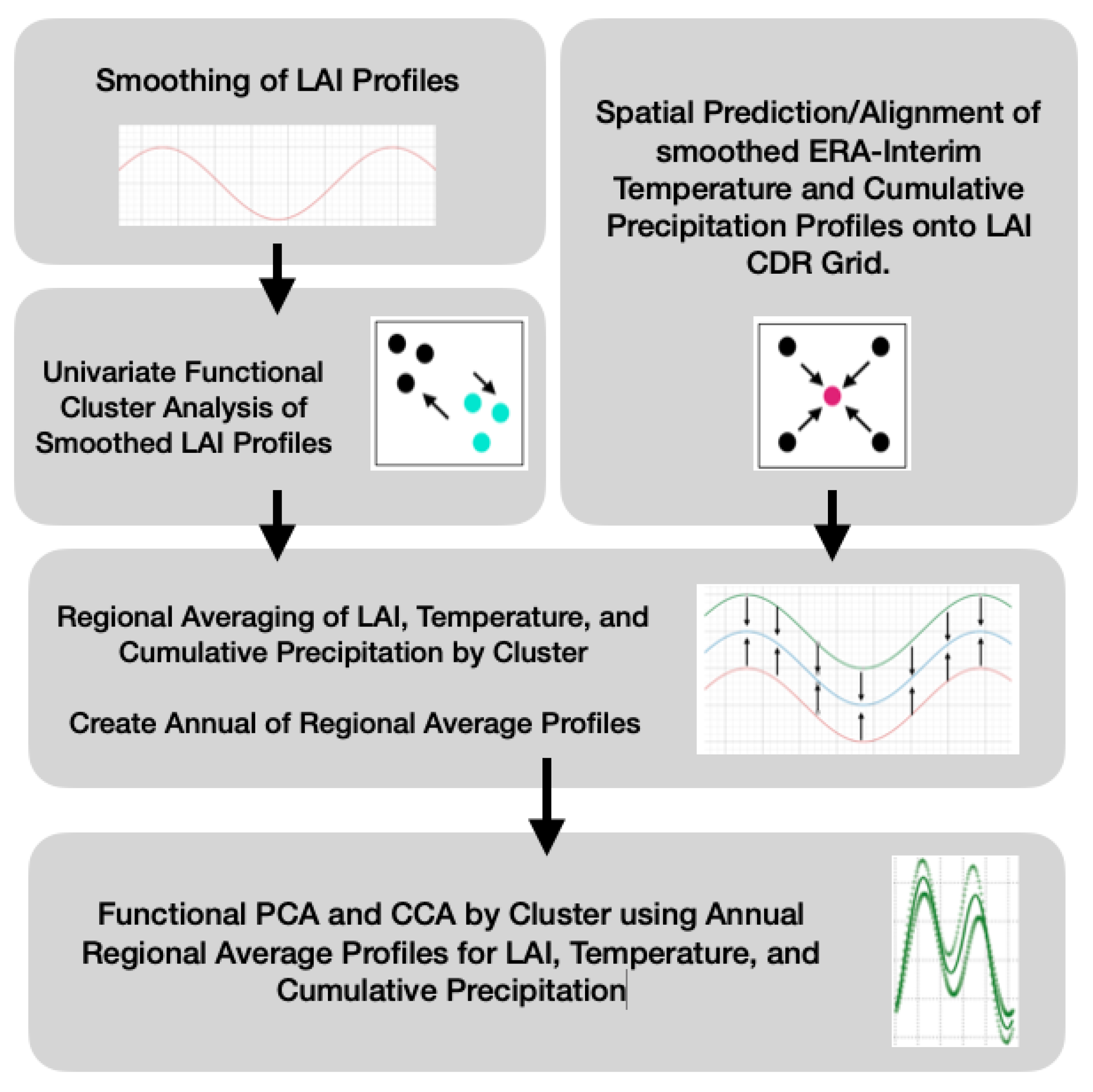
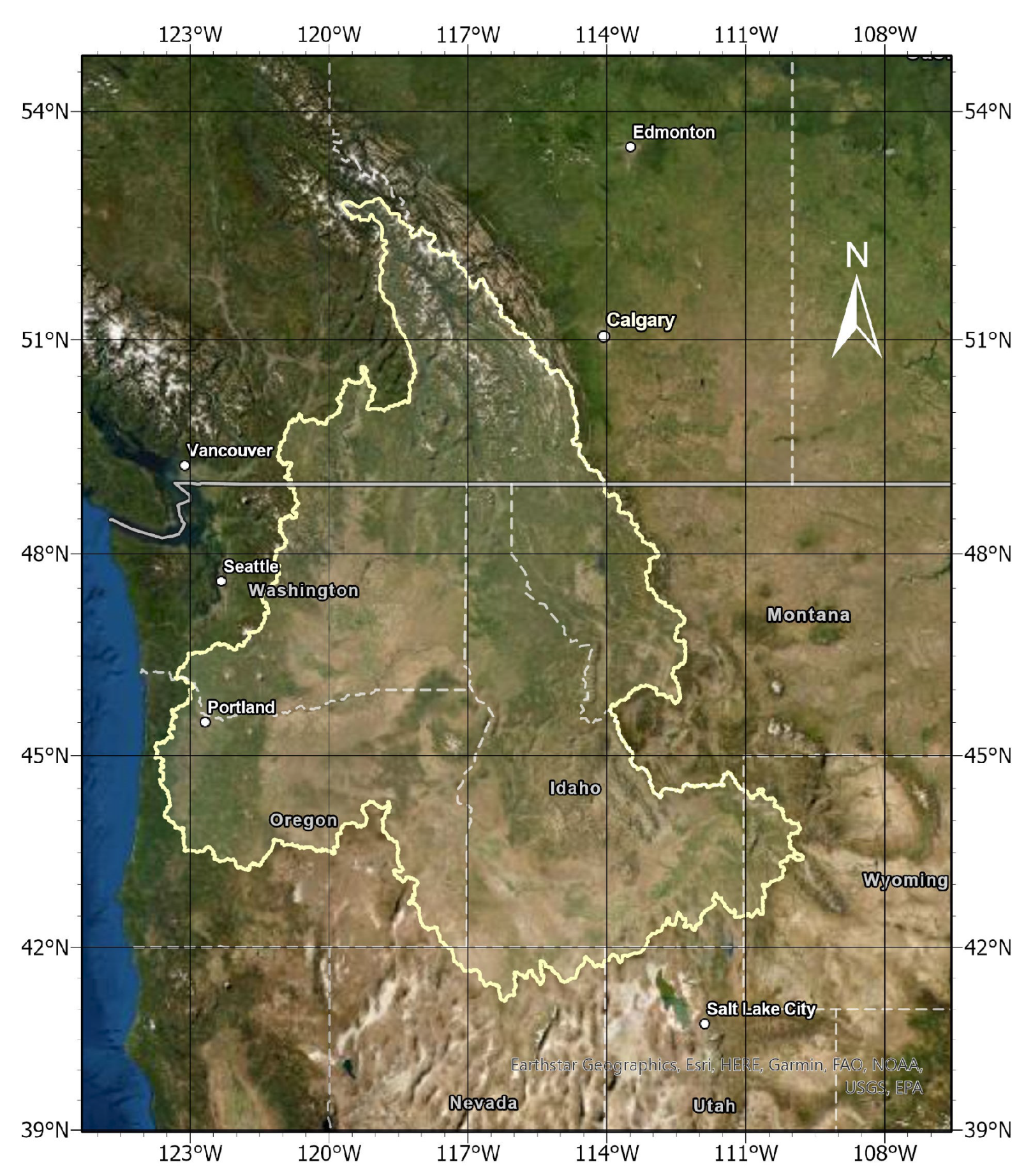
In this study, the Columbia River Basin (CRB) region of the Northwestern United States was chosen to explore the use of FDA for analyzing vegetation dynamics over multiple decades and correlating vegetation dynamics to changing climate conditions. The objective of this research is to demonstrate the potential of FDA to analyze remotely-sensed vegetation and climate data and provide insight on the effects of changing climate conditions on plant life across a diverse set of ecoregions in the CRB. To do this, we constructed smoothed-spline estimates of LAI from 1996 to 2017 using the remotely-sensed NOAA Advanced Very High-Resolution Radiometer (AVHRR) time series product. We then developed a functional cluster analysis model to allocate 27,196 sites in the CRB into more uniform groups based on similar trends in LAI. Next, we took regional averages of those groups and investigated intra- and inter-annual variability in vegetation dynamics within each cluster. Finally, we used a climate data product from the European Centre for Medium-Range Weather Forecasts global atmospheric re-analysis (ERA-Interim) to determine correlations between intra- and inter-annual vegetation dynamics and temperature and precipitation in each cluster.

2. Materials and Methods

This work integrates an array of methods and data products. At the end of this section, Figure 1 summarizes the full modeling process as a flow diagram. The complete model visualized in this image outlines the general guidelines resulting from this work for smoothing, grouping, and averaging of vegetation data and spatial alignment/prediction of other relevant data onto a matching spatial grid. The general modeling process of this work is highly flexible in the sense that there are several statistical tools available for smoothing or interpolating continuous process, and there are many dissimilarity measures, distance metrics, and clustering methods available that could be implemented in a similar manner. The clustering model proposed in this work can also be used as a pre-processing step prior to a predictive modeling or forecasting analysis.

2.1. Study Region

The Columbia River Basin is located in the north-western United States and south-western British Columbia, Canada as shown in Figure 2. The drainage basin is bounded by the Rocky Mountains to the east and the Cascade and Coast range to the west and cover an area of 670,000 km2: 568,000 km2 of which is spread across the US states of Washington, Oregon, Idaho, Montana, Wyoming, Utah, and Nevada. Climate in the CRB varies from humid and maritime along the western parts of the basin to semi-arid and arid in the southeast. The CRB hosts a range of diverse natural ecosystems as well as large agricultural regions consisting largely of forestry, dairy and cattle farming, and production of apples, potatoes, wheat, and other small grains. (USGS River Basins of the United States: the Columbia report).

2.2. LAI AVHRR Climate Data Record

The LAI Climate Data Record (LAI CDR) produces a daily product on a 0.05 degree × 0.05 degree grid dating back to 1981 derived from AVHRR sensors using data from eight NOAA polar orbiting satellites: NOAA-7, -9, -11, -14, -16, -17, -18 and -19. The highest resolution of AVHRR sites is approximately 1 km per pixel [18,19]. In this analysis, we subset the data from 1 January 1996 until 31 December 2017 and the spatial domain is restricted to 37,110 sites in the US portion of the CRB (refer to Figure 2). In this 22 year period, daily LAI measurements are summarized on a weekly resolution, by taking the weekly average LAI across a 7 day period. The resulting data product has 1152 weeks. We chose to take weekly averages because of the regular occurrence of missing values at daily resolution and this is justified by the stability of vegetative processes from day to day. In this product, there are still thousands of sites that report high volumes of missing values. In order to construct spline smoothed curves on the 22 year period, a minimum threshold was set for 28 percent of weeks in the 22 year period to have at least one weekly recording of LAI. This filtering process leaves 27,196 sites. By inspection, we found that many of the removed sites were barren/sparsely vegetated regions and high altitude sites, and it is clear that there are some spatially-systematic errors in recording LAI.

2.3. ERA-Interim Reanalysis

The ERA-Interim is a reanalysis of the global climate attributes covering the data-rich period since 1979 (originally, ERA-Interim ran from 1989, but the 10 year extension for the period 1979–1988 was produced in 2011), and continuing in real time until its discontinuation in 2019 [20]. The spatial resolution of the data set is approximately 80 km and provides daily recordings of maximum temperature, minimum temperature, and precipitation. The product used in this analysis has been pre-processed into longitudinal attributes of these climate attributes by Jupiter Intelligence (for the American Statistical Association’s (ASA) Section on Statitics and the Environment (ENVR) 2021 Data Challenge). This product is subsetted temporally to the same domain prescribed for the LAI CDR. The spatial domain for this product is restricted to a square region containing the subsetted points from the LAI CDR with the following boundaries ( L a t m i n = 40.5 N, L a t m a x = 49.0 N, L o n m i n = 108.0 W, L o n m a x = 124.0 W). Requiring that the subsetted LAI CDR product fully contained within the subsetted ERA-Interim product is optimal for appropriate spatial prediction of climate attributes of the ERA-Interim product onto the LAI CDR coordinate system.

2.4. BaseVue 2013 Land Cover and USGS National Elevation Products

The results of the cluster analysis prompted further investigation into site characteristics that may be driving factors in the separation of clusters. We use the BaseVue 2013 Land Cover product, which is a commercial global, land use/land cover product developed by MDA [21,22]. BaseVue is independently derived from approximately 9200 Landsat 8 images and has a spatial resolution of 30 m. The capture dates for the Landsat 8 imagery range from 11 April 2013 to 29 June 2014, and contains 16 classes of land use/land cover. Elevations were extracted at each site using the USGS National Elevation product. This dynamic image service provides numeric values on a 30 m resolution representing orthometric ground surface heights (sea level = 0) which are based on a digital terrain model (DTM).

2.5. Smoothing LAI

For a collection of raw weekly average recordings of LAI, denoted by Y = [ y 1 y n ] , where y i is a vector of values discretely representing a continuous process, we estimate x ^ ( t ) = k = 1 K c k ϕ k ( t ) subject to a roughness penalty on the second derivative of the basis expansion Φ = [ ϕ 1 ( t ) ϕ K ( t ) ] , where c k are the coefficients of the terms of the basis expansion denoted by ϕ k . This can be expressed as an unconstrained minimization defined by
m i n c y Φ c 2 + λ c T R c f o r λ 0 ,
where R j k = l = 1 M ϕ j ( t l ) ϕ k ( t l ) h for h = t l t l 1 [11]. The value M is the number or time points on a fine time grid t 1 , , t M . The λ parameter is a tuning parameter that restricts the roughness of the spline model as λ increases in magnitude. The resulting smoothed LAI curves have the form
x ^ = Φ ( Φ T Φ + λ R ) 1 Φ T y = S y .
We select an appropriate value for λ coordinates using the optimal λ for a single site determined by the generalized cross-validation criteria,
G C V = M S E ( λ ) ( 1 d f λ M ) , w h e r e
d f λ = t r a c e ( S )
The GCV criterion is derived from the mean-squared error penalization criterion for the spline model defined by
M S E ( λ ) = y Φ c 2 M d f λ
The roughness of LAI recordings at all sites is similar, and our choice to fix the roughness penalty restriction permits the estimated functions to characterize the same types of features across coordinates in the Columbia River Watershed. In the upper plot of Figure 3, we present an example of a smoothed 22 year LAI profile. The time domain consists of 1152 weeks. The spline models are constructed with 385 equally spaced knots and 387 basis functions. The basis functions used to construct spline models for each site are cubic B-splines (second-order polynomials). We emphasize that the curves retain the timing and structure of the raw data while naturally filtering out singleton anomaly values that yield false maximum LAI readings.

2.6. Spatial Clustering of Univariate High-Dimensional Functional Data

In this section, we propose the functional clustering model implemented in this project. The objective of a cluster analysis is to separate observational units (sites) into more homogenized groups. The derived groups can be studied separately given that the clustering model is verified to have an appropriate structure. In this work, we aim to study changes in regional average LAI profiles by taking averages of the smoothed LAI profiles from each site in a given cluster. The clustering model provides the critical step in ensuring that we are only averaging profiles together that are structurally similar.
Consider each smoothed curve, x j ^ ( t ) as a vector of measurements. Although spline models are continuous functions that have infinite values on their domain, the models must be represented with a refined time grid that is measured discretely, but preferably finer than the raw data from which the spline models are derived. In this work, the time-mesh for the spline models is twice the weekly resolution of the original LAI CDR. Since the original data in this work is recorded weekly for 1152 weeks, this implies that the time grid for the smoothing splines is 2304 points. The pairwise correlation of x ^ j ( t ) with x ^ j ( t ) can be measured by plotting the two curves against each in R 2 . Plotting smoothed LAI curves in this way yields ellipsoidal paths of time-paired LAI recordings ( x ^ j ( t i ) , x ^ j ( t i ) ) . We measure the strength of monotonicity of the ellipsoidal relationship of coordinates rather than its linearity. To accomplish this, we compute Spearman rank correlations defined by
ρ ( x ^ j , x ^ j ) = ρ j j = S x ^ j x ^ j S x ^ j S x ^ j = n 1 n [ R ( x j ) R ( x j ) ¯ ] [ R ( x j ) R ( x j ) ¯ ] n 1 n [ R ( x j ) R ( x j ) ¯ ] 2 · n 1 n [ R ( x j ) R ( x j ) ¯ ] 2
between all pairs of coordinates, where R ( x j ) is the ranking function of the elements of x ^ j ( t ) . This approach proves advantageous in this application since Spearman correlation is a computationally efficient measure of association for a high dimensional quantities of paired coordinates. This approach also provides a notion of standardization of the measure of association which is of great application-based importance, namely that coordinates grouped in the same cluster have increasingly synchronous greening patterns independent of the differences in the magnitude of LAI at each site. As an example, coordinates on north-facing slopes may experience lower and seasonally delayed LAI than south-facing slopes, but if close enough in proximity, the regularity of paired ellipsoidal LAI movement in R 2 will likely be high.
The ρ j j can be thought of as a discretization of a spatial correlation function P, where ρ j j = P ( x j , x j ) . The availability of longitudinal recordings of LAI at each coordinate allows for direct estimation of ρ j j without placing assumptions on P [25]. The computed n × n matrix of pairwise correlations is used to construct a dissimiliarity matrix with elements d j j = 1 ρ j j .
By construction, pairs of coordinates with high Spearman correlation have low d j j values, and as such, they are considered to be close in “distance” to each other. We then perform k-mediod clustering using the partitioning around mediods algorithm (PAM) for k = 2 , , 6 clusters [26]. There are other dissimilarity metrics for functional data available such as integrating the difference of two functions, dynamic time warping (DTW), and information theoretic measures [27,28,29]. Ultimately, exploring a large selection of dissimilarity metrics is left to future work. Our choice in this work to select a computationally efficient and simple measure of dissimilarity is rooted in our effort to use the simplest tool that can detect the differences in functional structure of spline models while also considering the extension of our work to larger remote-sensing data products.

2.7. Ordinary Functional Kriging of the ERA-Interim

In this work, we seek to relate any detected structure in the smoothed LAI profiles derived from the LAI CDR to atmospheric variables. We use the ERA-Interim data to accomplish this objective. Since the ERA-Interim reanalysis product is on an 80 km resolution, spatio-temporal prediction onto the LAI CDR grid is required. This is accomplished using Ordinary Functional Kriging on the ERA-Interim. Considering a functional random process { X S : s D R d } with d = 2 such that X S is a functional random variable for any s D observed at n sites [30,31]. It is assumed that the random process is second-order stationarity and isotropic. We predict a complete smooth function X ^ S 0 : [ a , b ] R , expressed by
X ^ S 0 = i = 1 n λ i X S i , λ 1 , , λ n R .
By construction, X ^ S 0 is a linear combination of observed curves with weights λ 1 , , λ n R . Curves from locations closer to the prediction site are constructed to have increased influence on the prediction. We use a parametric estimated trace-semiovariongram with the exponential distribution to obtain the kriging weights λ i .

2.8. Deriving Regional Average Profiles

From Section 2.5, we have obtained smoothed LAI profiles { x i L ( t ) | i = 1 , , 27 , 191 } , and from Section 2.7, we have obtained smoothed temperature and cumulative preciptation profiles { x i T ( t ) | i = 1 , , 27 , 191 } and { x i P ( t ) | i = 1 , , 27 , 191 } . The functional cluster analysis model proposed in Section 2.6 is used to average site profiles by cluster. The averaging by cluster can be represented by
μ ^ L ( j ) ( t ) = n 1 i = 1 n x i L ( j ) ( t ) ,
μ ^ T ( j ) ( t ) = n 1 i = 1 n x i T ( j ) ( t ) ,
μ ^ P ( j ) ( t ) = n 1 i = 1 n x i P ( j ) ( t ) ,
where j corresponds to the j t h cluster from the functional clustering model, and n is the number of sites in the j t h cluster.

2.9. Inter-Annual Regional LAI and Climate Variation Monitoring

Prior to this section, we have obtained regional averages of smoothed LAI profiles, maximum temperature, and cumulative precipitation profiles by cluster from 1996 to 2017 predicted onto the 0.05 × 0.05 degree grid. We separate each of the average profiles μ ^ L ( j ) ( t ) , μ ^ T ( j ) ( t ) , μ ^ P ( j ) ( t ) into a collection of 22 annual curves defined by
μ ^ ( j ω ) ( t ω ) = i = 1 n x i ( j ω ) ( t ω ) ,
where { t ω | t ( 1 / 01 / ω , 12 / 31 / ω ) , ω = 1996 , 2017 } . The deconstruction into annual curves provides the needed replications of curves to assess inter-annual variation using functional principal components analysis (FPCA) and functional canonical correlation analysis (FCCA). The collection of average profiles, μ ^ ( j ω ) ( t ω ) , for either LAI, temperature, or precipitation is then investigated using FPCA.
For a given collection of average annual profiles for a given cluster LAI, denoted by { μ ^ ( j ω ) ( t ω ) } which are realizations of the the random function X ( t ) , and the Karhumen–Loeve decomposition of the annual profiles can be expressed using the random variable Z defined by
X ( t ) = μ ( t ) + k = 1 z k ξ k ( t ) ,
where μ is the known average profile of the 22 annual curves μ ^ ( j ω ) ( t ω ) for all ω , the ξ k are orthonormal eigenfunctions that characterize variance of individual years, ω , from the mean, and the z k are uncorrelated random variables such that E ( z k ) = 0 and V ( z k ) = λ k , where λ k is the eigenvalues corresponding to the k t h eigenfunction [11,12]. The eigenfunction pairs ξ k , known as functional princpal components (FPCs), are the leading eigenfunctions of the functional covariance defined by v ( s , t ) = ω 1 i = 1 ω ( μ ^ ( j ω ) ( s ω ) μ ¯ ( j ω ) ( s ) ) ( μ ^ ( j ω ) ( t ω ) μ ¯ ( j ) ( t ) ) and z k is an eigenvector of the Gram matrix G, defined by G ω ω = < μ ( j ω ) μ ¯ ,   μ ( j ω ) μ ¯ > with eigenvalues ω λ k .

2.10. Inter-Annual Canonical Correlation Analysis between LAI and Climate Attributes

The FCCA procedure is outlined using regionally averaged annual LAI and temperature profiles. Consider a sample of paired annual curves { ( μ ^ L ( j ω ) ( t ω ) , μ ^ T ( j ω ) ( t ω ) ) } where each annual LAI curve for a given year ω has a matching annual temperature profile for year ω . Let x ω = μ ^ L ( j ω ) ( t ω ) be realizations of the random function X, and y ω = μ ^ L ( j ω ) ( t ω ) be realizations of the random function Y. The objective is to discover functions ( ξ , η ) that maximize c o r ( < x ,   ξ > ,   < Y ,   η > ) . Defining Z = < ξ ,   X > and W = < η ,   Y > , gives
ρ = c o r ( Z , W ) = c o v ( Z , W ) V ( Z ) V ( W )
where
V ( Z ) = a b a b c o v ( X ( s ) , X ( t ) ξ ( s ) ξ ( t ) d s d t = < ξ , c o v ( X ( s ) , X ( t ) ) ξ > , V ( W ) = a b a b c o v ( Y ( s ) , Y ( t ) η ( s ) η ( t ) d s d t = < η , c o v ( Y ( s ) , Y ( t ) ) η > , c o v ( z , w ) = a b a b c o v ( X ( s ) , Y ( t ) ξ ( s ) η ( t ) d s d t = < ξ , c o v ( X ( s ) , Y ( t ) ) η > .
In this work, we only focus on the first pair of canonical correlation weight functions. Subsequent canonical weight functions can be found, but the details of this procedure are not provided [11].
FCCA requires some form of regularization to ensure meaningful weight functions ( ξ , η ) since they only have m constraints but as functions have infinite degrees of freedom (unlike classical CCA) [11]. This is accomplished by defining the smoothed sample curves using the first four functional principal components of X and Y as the basis expansion as opposed to a standard b-spline basis expansion. The FPCA models have shown that the first 4 FPC’s explain 90 to 99 percent of the variability of the original sample and are expressed by x ω ( t ) = μ x + k = 1 4 s ω k ν k ( 1 ) and y ω ( t ) = μ y + k = 1 4 s ω k ν k ( 2 ) , where ν and s ω k are defined similarly to Equation (12).
The strength of the relationship between LAI and temperature or precipitation, ρ , provides the conventional interpretation of correlation, but equally important, the paired weight functions ( ξ , η ) are the components of variation that most account for the interaction of the two attributes.

3. Results

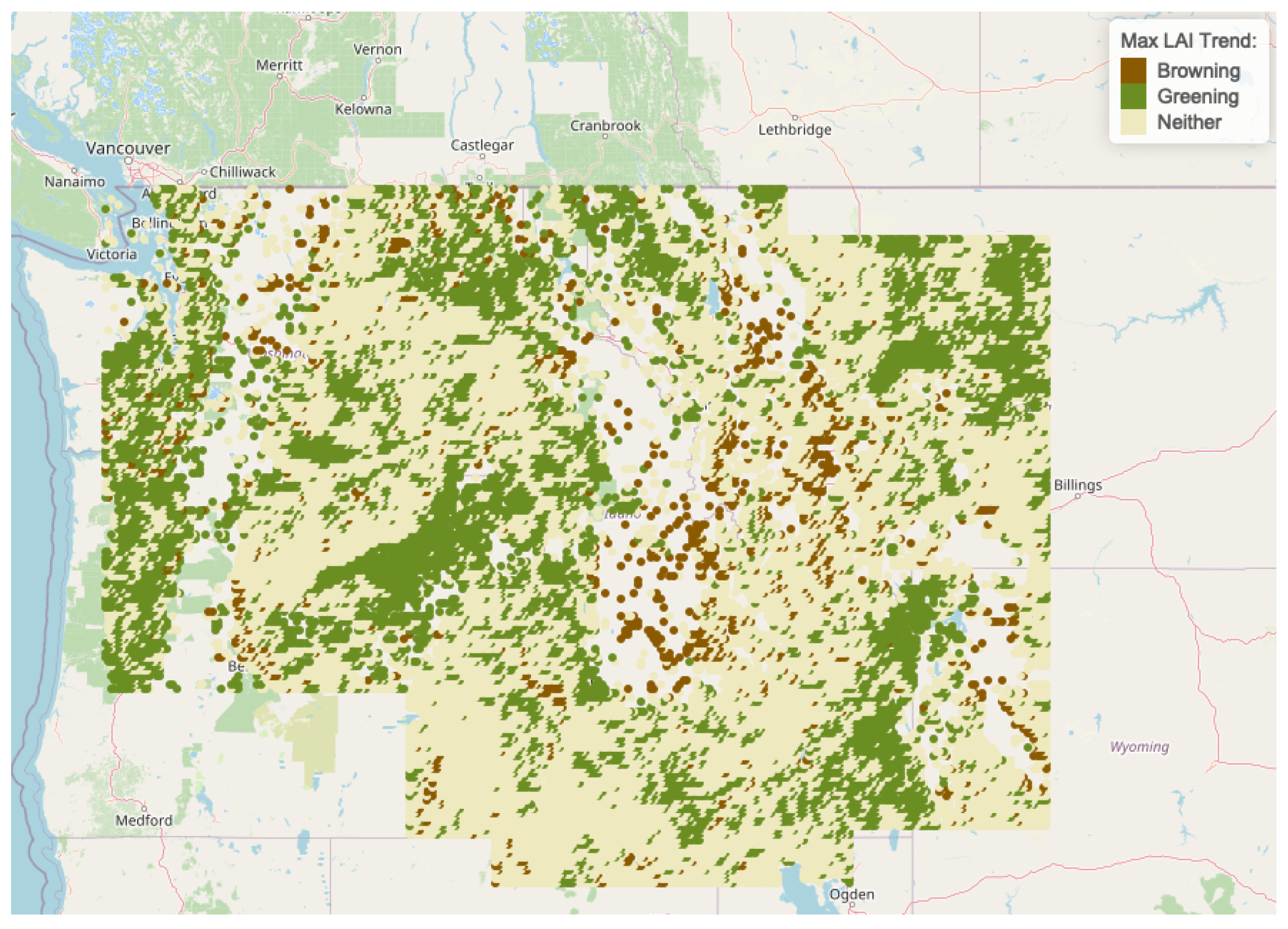
This analysis detects widespread greening earlier in the growing seasons across diverse areas in the CRB from 1996 to 2017. Initial exploration of correlations between annual maximum LAI and time in this region provide evidence of this phenological shift. Figure 4 and Table 1 and Table 2, show calculated correlations between detected annual maximum LAI at each site and time (measured in years). To be explicit, correlations are calculated at each site for 22 years with respect to 22 annual maximum LAI measurements. These are computed from the raw data in the LAI CDR. Significant correlations were determined at α = 0.15 . Sites are referred to as “greening sites” if they have significant positive correlations between LAI and time, whereas sites with significant negative correlations between LAI and time are referred to as “browning sites.” Non-significant correlations are denoted as “Neither” greening nor browning. High frequencies of greening were detected along large sections of the the major CRB rivers (the Columbia and Snake) and in the Pacific coastal region of the CRB. Generous significant levels were chosen in this preliminary stage since, with only 22 replications of annual maximum LAI (over the 22 years), the correlation coefficients are sensitive to anomaly measurements and sub-intervals of decreasing annual maximum LAI. A high anomaly reading in early years makes it difficult to detect an increasing trend across the remaining years. Further, a sudden drop in maximum LAI in later years may leverage the correlation away from a high positive correlation detected in earlier intervals.
The spatial distribution of greening magnitude and timing demanded a more rigorous exploratory analysis that accomplished the following objectives: (1) eliminate/filter anomalies (false high LAI recordings), (2) detect regions that are strongly correlated over time while retaining at least some information regarding spatial proximity, and (3) examine changes/perturbations in the functional structure of annual LAI profiles.
The proposed functional clustering model was implemented on the 22 year smoothed LAI profiles using the dissimilarity matrix outlined in Section 2.6. Sites allocated into the same cluster are determined to have strong multidecadal relationships to each other as inherited from the dissimilarity matrix. 
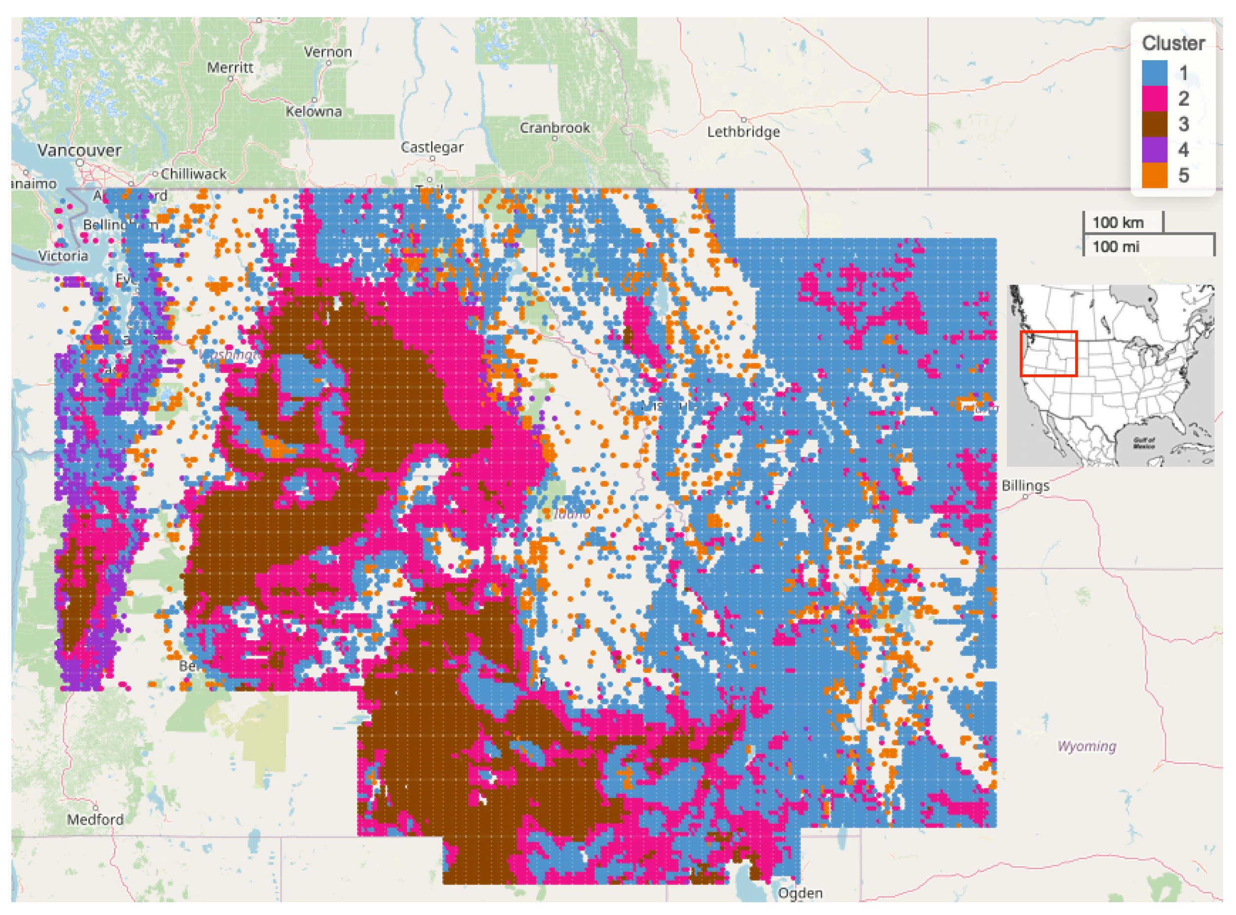
Figure 5 depicts the results of the 5 cluster k-mediods model geographically. The details of the all cluster models for k = 5 are provided in Table 3. We selected k = 5 primarily because the yielded cluster sizes were sufficient for regional-scale inferences. The differences in regional average LAI profiles by cluster provided exceptional separation by the timing, magnitude, and number of annual peaks in LAI. The geographic shape of the clusters also follows many major geographic features in the region, such as river basins and mountain ranges.
It becomes apparent that a simple naming or classifying of clusters is not achievable. Although there is significant separation of the clusters by land cover and elevation, there are clearly other regional or spatially confounding environmental factors separating these clusters. Recent work investigating these clusters has shown that site elevation, water storage potential, and terrain slope are the most important site attributes when predicting cluster allocation of sites [33].
The 5 clusters intuitively distinguish regions with different land cover, elevation, and climate characteristics based on satellite-derived LAI values. Table 1 and Table 2 show that across Clusters 1, 2, 4, and 5, 32–70 percent of sites are identified as greening sites, and extremely low percentages of sites in each cluster are identified as browning sites. 
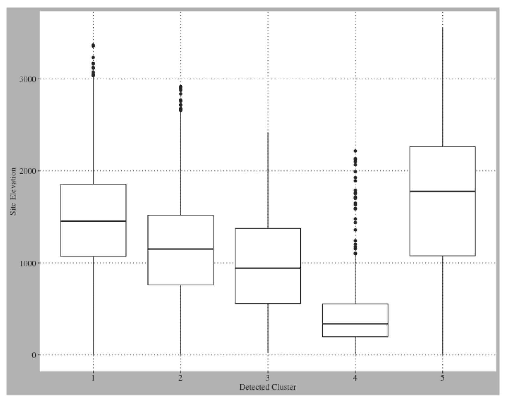
Table 4 shows the land cover classifications for each of the five clusters. Clusters 1, 2, and 3 contain the largest proportion of agricultural sites and the majority land cover classification for these 3 clusters is scrub/shrub. Clusters 4 and 5 are dominantly forested, evergreen sites. All clusters are distinguished by significant differences in elevation distributions, with Cluster 5 containing the highest elevation sites and Cluster 4 containing the lowest elevation sites (Figure A1).
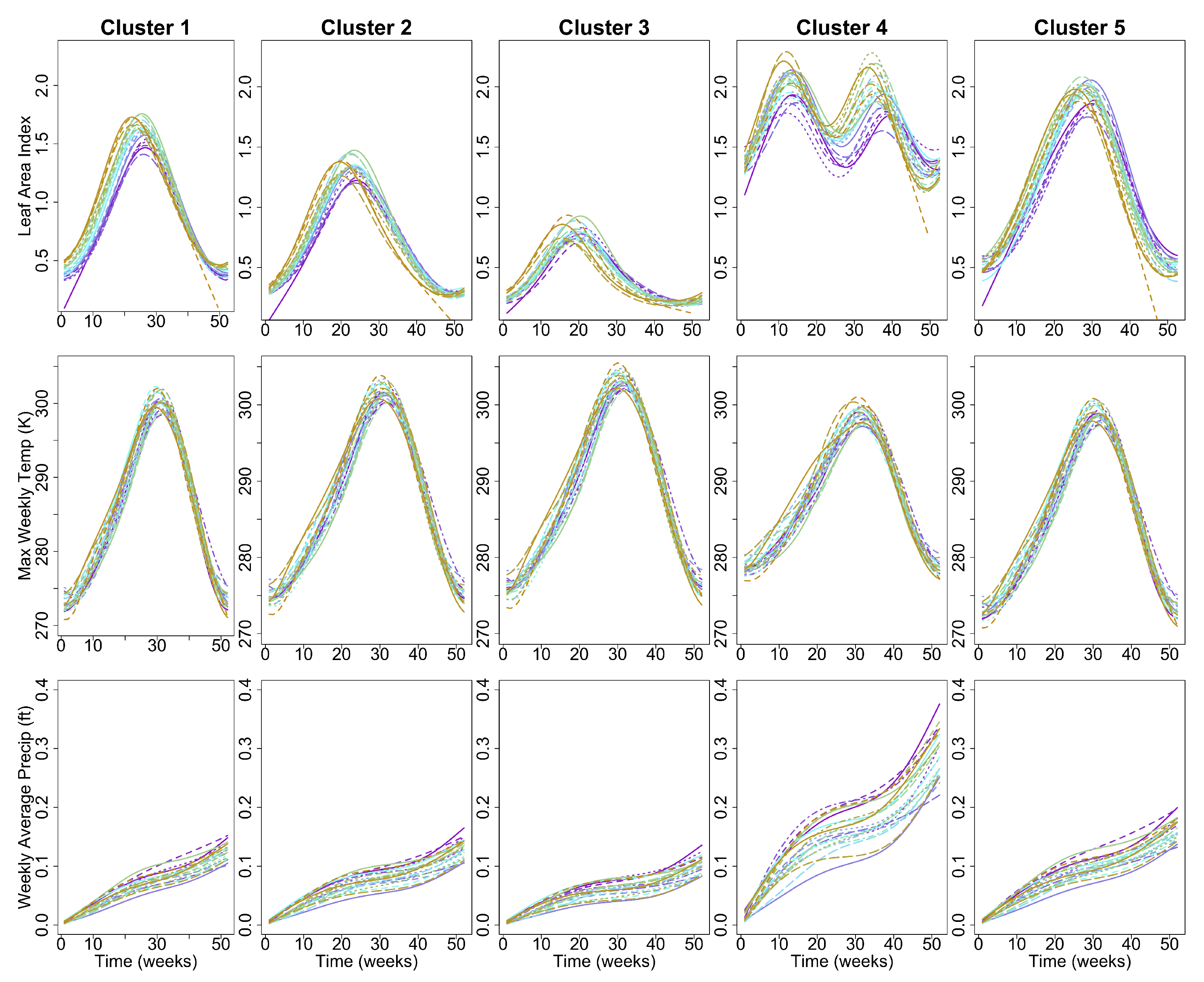
Figure 6 shows annual profiles for weekly maximum LAI, weekly maximum temperature, and average weekly precipitation for each of the five clusters. Annual maximum LAI is highest in the evergreen forested sites in Clusters 4 and 5 and lowest in Cluster 3, which contains sites with the highest proportion of scrub/shrub land cover in the CRB. Annual temperature profiles are similar throughout the CRB region, with slightly lower annual maximum and higher annual minimum temperatures detected throughout the 22 year time period at the low-elevation coastal sites comprising Cluster 4. Annual precipitation profiles are similar for Clusters 1, 2, 3, and 5, with Cluster 4 receiving much greater cumulative precipitation than the other clusters each year.
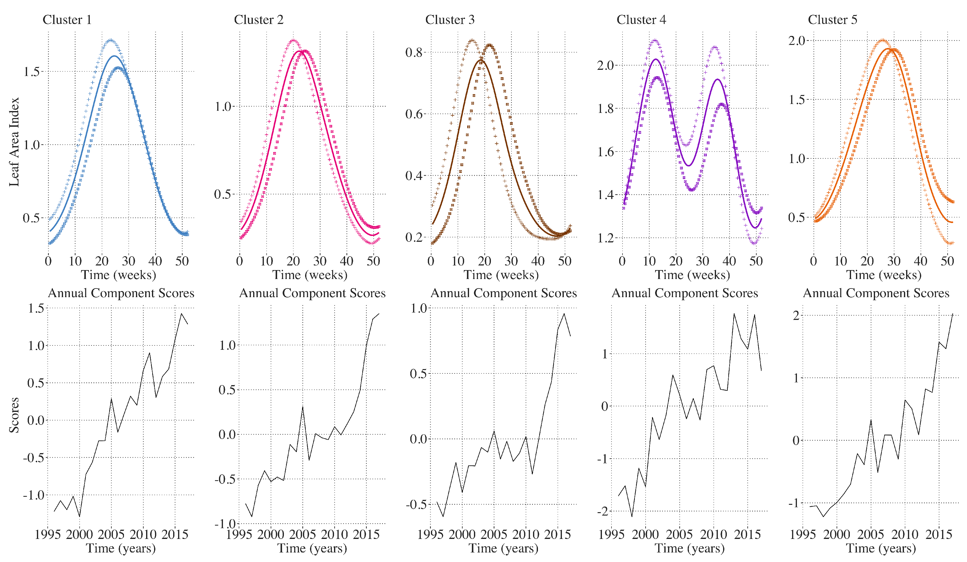
A brief summary of the FPCA results is presented in Table 5. In the FPCA of annual LAI profiles, among all of the clusters, 55–75 percent of the inter-annual variation is explained by the first principal component which is characterized by earlier and higher peaks in annual maximum LAI. This is shown in Figure 7. The linear increase in principal component scores over time indicates a trend toward earlier and higher annual maximum LAI throughout the CRB region. This demonstrates that despite differences in land cover, elevation, and annual precipitation profiles between the five clusters, a clear greening trend is detected over the 22 year period throughout the CRB. In 
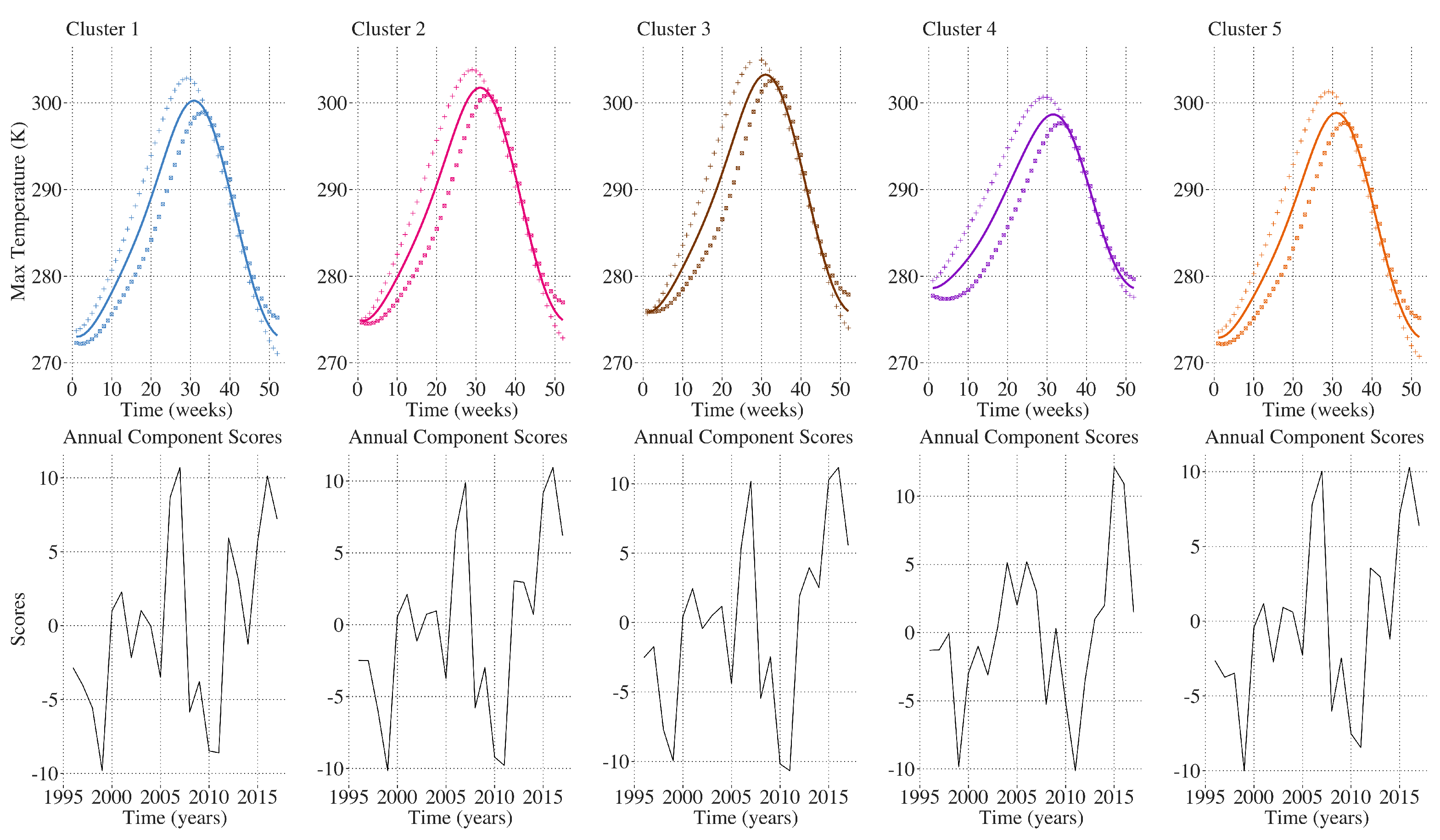
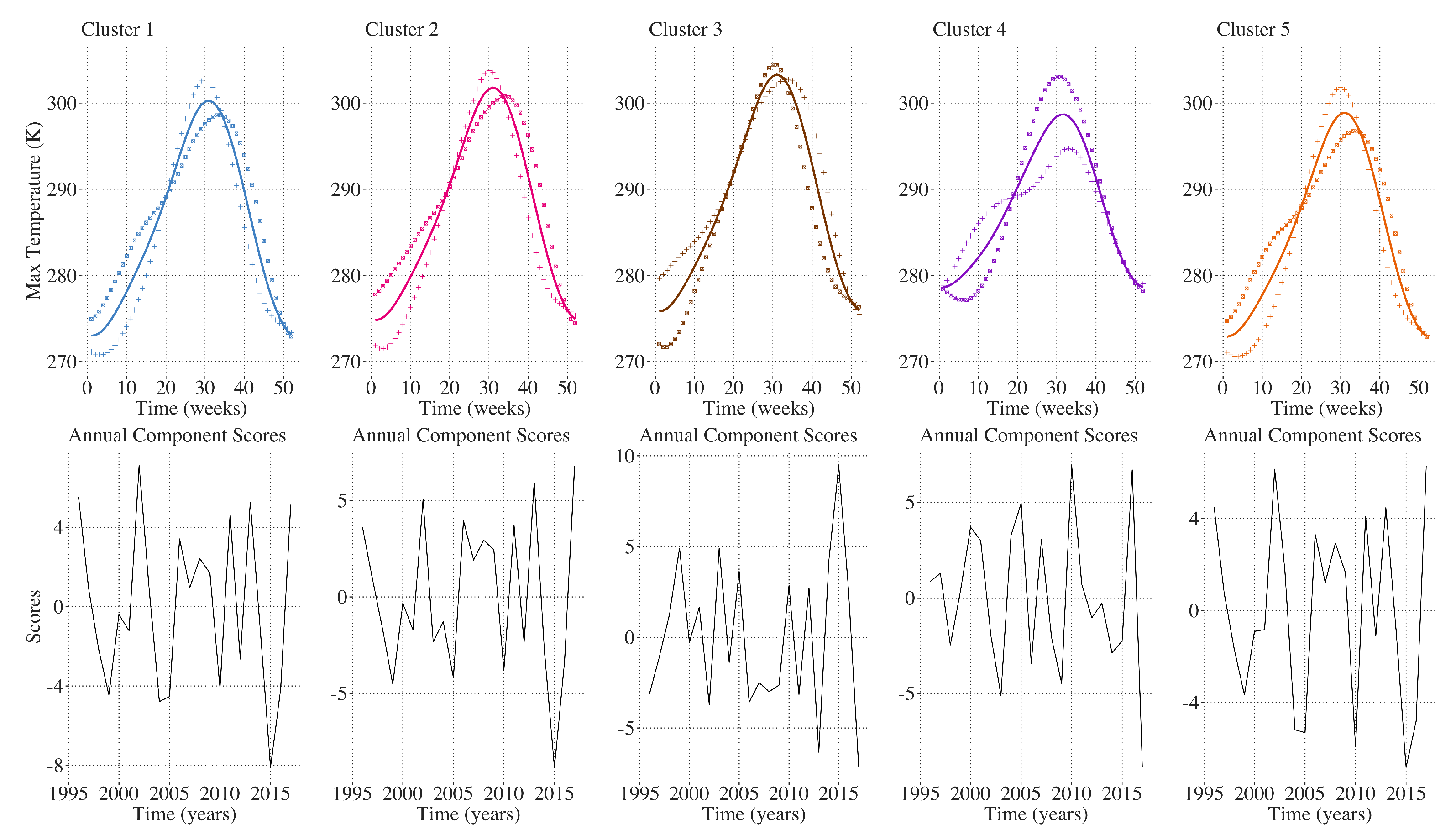
Figure 8, FPCA on temperature shows 45–48 percent of the inter-annual variability is explained by the first principal component which is associated with linearly warmer temperatures from the beginning of the year through the annual peak in summer temperatures. In Figure 9, the second principal component, explaining 20–23 percent of the inter-annual variability among the five clusters, is associated with either significantly warmer temperatures during the first 20 weeks of the year and a lower annual maximum temperature, or cooler temperatures during the first 20 weeks of the year and a higher annual maximum. In 
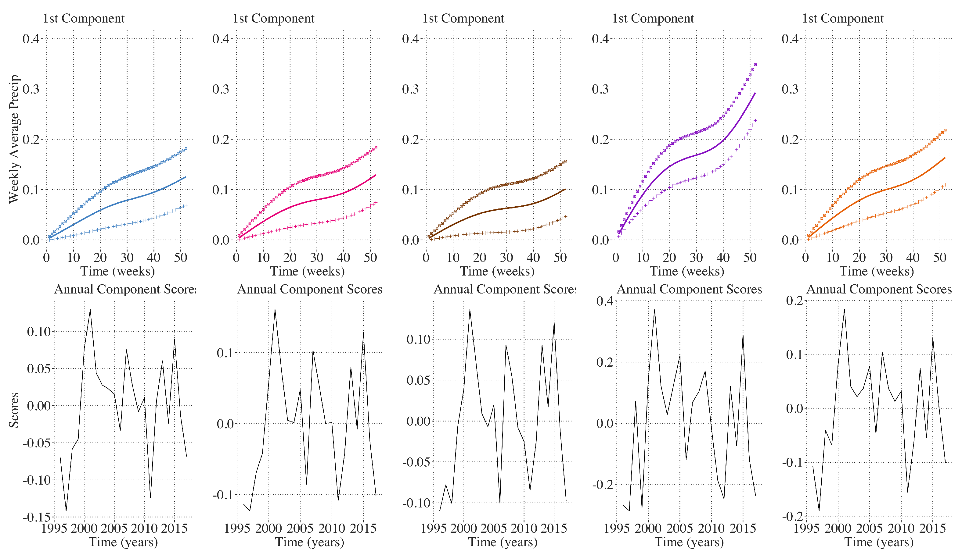
Figure 10, identical analysis on annual cumulative precipitation shows 90 percent of the inter-annual variation among all of the clusters was explained by the first principal component characterized by either greater or less annual cumulative precipitation. Annual maximum temperature and annual precipitation profiles do not demonstrate an obvious trend over the time period 1996–2017 (Figure 8 and Figure 10).
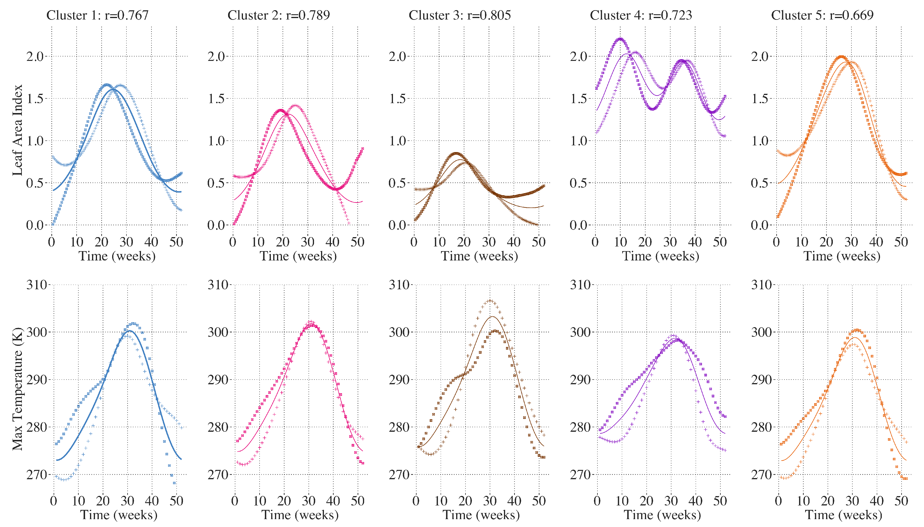
The FCCA reveals correlations between intra-annual variation in temperature and precipitation and the earlier and higher LAI peak being detected in each of the clusters. In each cluster, the shift in phenology toward earlier and higher annual maximum LAI values are correlated with warmer temperatures during the first 20 weeks of the year, shown in 
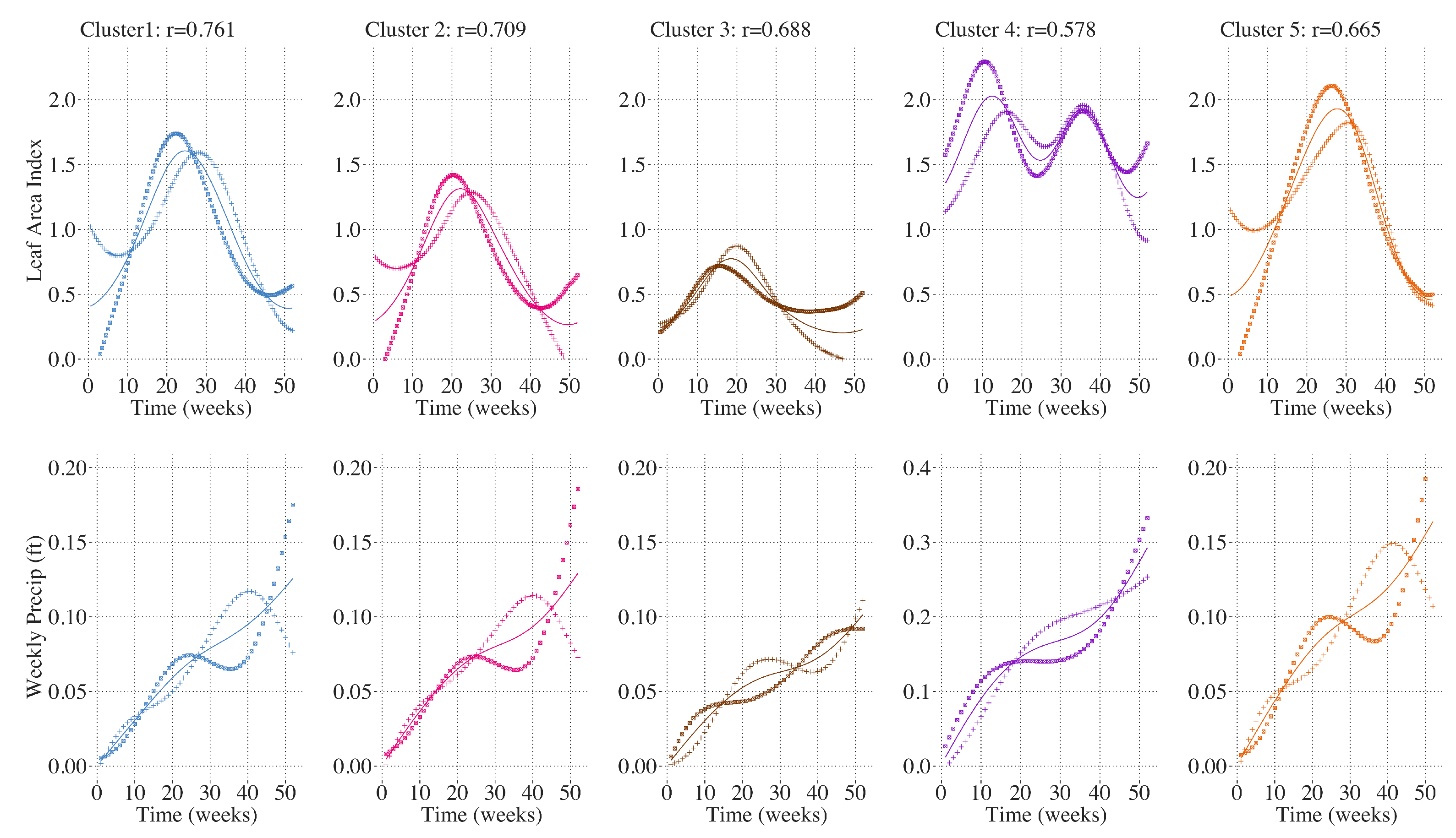
Figure 11. FCCA between LAI and precipitation did not yield a consistent correlation among the clusters. For Clusters 1 and 5, greater and earlier maximum LAI was correlated with large increases in cumulative precipitation in the winter and spring, and later and lower maximum LAI was correlated with greater accumulation in the late summer and early fall. Cluster 2 shows a similar trend except that the correlation between LAI and cumulative precipitation is most strongly driven by differences in fall and early winter where large accumulations of precipitation in the fall are more strongly associated with later and lower maximum LAI. For Cluster 3, greater but not earlier maximum LAI in Cluster 3 was also correlated with greater spring precipitation, shown in Figure 12. For Cluster 4, the first annual peak in LAI is associated with dryer summers and greater accumulation in the winter. Taken together, the results of the functional canonical correlations indicate that the widespread shift in phenology toward an earlier and higher peak in annual LAI in the CRB is largely associated with warmer temperatures early in the year. However, the differences in inter-annual trends in temperature and LAI over the studied time period suggest there are other drivers of the trend in LAI not captured in this analysis. Greater annual maximum temperatures are not as strongly correlated with this shift in LAI and the correlation between annual precipitation and the timing and magnitude of the annual LAI peak varies between the 5 clusters.

4. Discussion

The results of this work demonstrate the utility of FDA for the detection of annual greening trends of high dimensional data of phenological processes, and more specifically, the characterization of the within-year and across-year trends in vegetation dynamics. Annual greening of field measured or remotely-sensed sites is best characterized by multiple parameters, namely the magnitude of the peak “greenness”, the (annual) timing of the peak, the duration of greeness, and the point of maximum change in greenness. Although only the first and second of these parameters are examined in this analysis, all of these features are inherently contained in the sample of 27,196 smooth functions used in this study. Any future work to examine the other features of LAI curves can be performed using the same preprocessing used here. Without the use of spline smoothed LAI curves, the analysis of these individual parameters must be assessed without the same theoretical cohesiveness present in this approach. Ultimately, annual LAI profiles are simple to smooth, and we demonstrate that variation in annual LAI across years is effectively detected and explained using functional principal components analysis.
We believe that the modeling of processes with underlying continuity should take advantage of this continuity when possible. In this analysis, we demonstrate that the modeling of continuous processes in the presence of high volumes of missing values is achievable, and our results lead us to believe that our choice to only consider sites with less than 72 percent missing values is conservative, and such an analysis would be effective with upwards of 80 percent missing values. This provides opportunities to use such methods in regions where remotely-sensed greenness indices are recorded with extreme sparseness, such as boreal, and Arctic climates [7]. We must acknowledge disadvantages of our sampling of sites in the region. First, the quality of the LAI AVHRR CDR has improved across its entire domain from 1982 to present. Beginning in 1996 eliminates some of the years with the lowest quality, but it is possible and likely that we have removed sites that had improved satellite coverage in the later years of the domain. Also, we note that the removal of most sites along the Montana–Idaho border and mountains of Oregon and Washington is not indicating low greenness but rather poor coverage through a substantial portion of years in our study.
Our clustering approach used in this project is effective at separating regions intuitively across an array of variables (land cover, elevation, temperature, and precipitation) with only the use of satellite-derived LAI profiles. We have conducted a deeper investigation of cluster allocation by a larger array of environmental attributes in a secondary work, where we identify strong predictive relationships between elevation, water storage potential, and slope on cluster allocation [33]. The clustering approach in the present study provides the theoretical framework to make regional inferences about changes in climate and greenness. The approach is proficient for analyzing tens or hundreds of thousands of sampled sites without parallel processing or high-performance computing (HPC). Future implementation of this approach using HPC would allow for investigation of regions far greater than the CRB.
Although our cluster model retains some implicit use of proximity of sites (since closer sites have a tendency to have higher correlations), we believe that there are necessary improvements to such a clustering approach, namely the filtering of noise sites (using methods such as DBSCAN) and inducing a spatial weighting (or penalization) on the dissimilarity matrix used in our work. We argue that the merits of the approach taken justify its presentation here, and we encourage further work in unsupervised learning methodology of phenological processes.
We emphasize that our work here is strictly exploratory, and not predictive. The relationships between climate and LAI discussed here are associative by nature, and further work using functional regression models is required to explore the fascinating predictive relationship between these attributes. Recent literature implementing predictive modeling of FPCA scores of NDVI has yielded promising results, and this approach can be extended to model climatic factors (such as CO2 concentration, Gross Primary Production, plant respiration, soil moisture) that predict higher FPCA scores for LAI in recent years in this region [14].
Our work is also insufficient without recognizing disadvantages of the LAI CDR using AVHRR sensors [34,35,36]. Recent literature has shown that this product is lesser to Moderate-Resolution Imaging Spectroradiometer (MODIS) sensors in making valid inferences on field measurement resolution and areas with higher annual precipiation (>1 m) [37,38]. As shown in Figure 6, regional cumulative precipiation averages for all clusters are well below this threshold. We add our work to the body of literature on the detection of changes in remotely-sensed greening, and we emphasize that the methods used in this project are directly extendable to any remotely-sensed time series data.
Numerous studies investigating remotely-sensed vegetation dynamics have reported a “greening” of the planet over the last several decades, attributed to multiple factors including the “fertilization effect” of higher atmospheric [CO2], nitrogen deposition, or increasing temperatures lengthening the growing season in many regions [39,40,41]. In this analysis, we were able to detect such a “greening” across a range of land cover classes and ecosystem types in the CRB of North America from 1996 to 2017. The shift in vegetation dynamics toward earlier and higher annual LAI peaks indicates changes in plant phenology across this region over the studied time period.
Plant phenological events in temperate regions are triggered predominantly by the well-known climatic changes associated with the changing of the seasons. These responses of vegetation to environmental conditions provide a measurable and accurate signature of the impact of climate change on plants [42]. The importance of understanding how plants respond to changing climate conditions has led to considerable work on the influence of climate variables on plant phenology [43]. Our analysis investigates the intra-annual relationships between vegetation dynamics and the climate variables temperature and precipitation throughout the year over a multidecadal timescale. Temperature is the dominant driver of the timing of many plant developmental processes and phenological shifts [44,45,46]. Plants synchronize their growth and development with favorable thermal conditions in order maximize the growing season and minimize the risk of frost damage. Sufficient exposure to cold temperatures in the winter is required for many plants to break dormancy, and a subsequent accumulation of degree days in the spring (time above a given temperature threshold) triggers budburst and the unfolding of leaves [47].
In the present study, earlier and higher annual maximum LAI throughout the CRB was largely correlated with higher temperatures during the first 20 weeks of the year. Phenological responses to environmental conditions can vary significantly among different regions and plant species [48,49]; however, similar trends in vegetation dynamics were found across a range of natural ecosystem and land cover types in the CRB, indicating common responses to abiotic environmental factors across the regional scale of this study. On agricultural land, spring planting date could influence the timing and magnitude of the peak in annual LAI. However, each of the 5 clusters contains a variety of land cover types and relatively small proportions of agricultural land. Because all of the clusters are showing coherent trends in LAI over the time period studied, the effect of differences in planting date on the agricultural fields in each cluster likely does not significantly influence the satellite-observed regional vegetation dynamics in the CRB.
The same intra-annual temperature trend was correlated with the earlier and higher maximum LAI values in each of the five clusters in the CRB. This result shows that greater accumulation of warm temperatures early in the year leads to an earlier onset of budburst and leaf unfolding, as well as an earlier peak of plant productivity in the summer growing season. Intra-annual trends in cumulative precipitation did not demonstrate a uniform correlation with the observed LAI trend among the five clusters in the CRB. This aligns with previous research that shows differential responses of phenology to precipitation between arid and wet regions and an overall lesser or indirect contribution of precipitation to plant phenological shifts compared to temperature [50,51].
A global warming trend of 0.2 degrees C per decade has been observed since the 1980s [52], and recent warming of the Northern Hemisphere, particularly in the winter and spring, is well documented [17,53,54]. Results of the functional principal components analysis on temperature in the CRB showed that greater than 60 percent of the inter-annual variability can be explained by warmer temperatures early in the year. Despite this, significant inter-annual variations in temperature trends exist across the CRB region between 1996 and 2017. Although warmer temperatures early in the year are seemingly the most important factor influencing the greening trend over time in this analysis, a clear trend toward early-year warming over the time period studied is lacking as shown by the lack of linearly increasing principal component scores for temperature over the 22 years. This indicates that while warmer spring temperatures are clearly influential over vegetation dynamics in the CRB, there are likely other factors playing important roles in the observed greening trend over time.
Vegetation dynamics in most plant species are mainly governed by temperature, photoperiod, precipitation, and the interactions among these key variables. The sensitivity of phenological shifts to these climate variables can differ among regions and plant species (especially sensitivities to photoperiod and precipitation [51,55,56]), and many of the underlying biological mechanisms that control phenological responses to these climate variables are still unknown. The influence of different climate variables have on plant phenology are entangled and the combined effects likely promote or constrain observed trends in vegetation dynamics [57,58]. For example, in mid and high latitude regions, warming temperatures in the spring are correlated with increasing day length. In photoperiod-sensitive plant species, early warming before a particular day length threshold is reached could constrain the temperature effect on spring phenology. Also, clouds associated with heavy spring precipitation could lower the sunlight intensity and quality and similarly constrain spring phenology. The timing of snowmelt is also an important factor in spring phenological shifts in regions with cold winters [59,60]. Warming early spring temperatures in regions near the CRB have been correlated with earlier timing of snowmelt [17], which is likely also correlated with the observed phenological shifts toward earlier greening.
Further investigation of the interactive and combined effects of climate variables on vegetation dynamics in the CRB is needed to fully understand the relationship between changing environmental conditions and observed trends in LAI.
The effect of globally increasing concentrations of atmospheric CO2 on vegetative growth should not be overlooked. Increases in anthropogenic emissions and land use change since the industrial revolution has driven the atmospheric CO2 concentration to over 400 parts per million (ppm), a approximately 40 percent increase since pre-industrial times [61]. Higher concentrations of CO2 in the atmosphere suppress the oxygenase activity of the main carbon-fixing enzyme in plants, ribulose 1,5-bisphosphate carboxylase-oxygenase (Rubisco). This leads to reduced rates of the carbon and energy dissipative process of photorespiration and increased photosynthetic carbon assimilation. While increasing concentrations of atmospheric CO2 are not found to change the timing of annual plant phenology [62], greening trends around the world have been attributed to the “fertilization effect” of increasing concentrations of atmospheric CO2 [39,63,64]. Though not investigated in the present study, increasing concentrations of atmospheric CO2 could play a role in the increasing magnitude of annual maximum LAI observed in the CRB.

5. Conclusions

The objectives of this study were to demonstrate the potential of FDA to analyze remotely-sensed vegetation and climate data and provide insight on the effects of changing climate conditions on plant life across a diverse set of ecoregions in the CRB. We did this by constructing smooth-spline estimates of remotely-sensed LAI from 1996 to 2017 across 27,196 sites in the CRB. We created a functional cluster analysis model to group sites with similar LAI profiles and then took regional averages of those groups to investigate trends in intra- and inter-annual variability within each cluster, and the correlations between temperature and precipitation and vegetation dynamics in each cluster. We then determined correlations between intra- and inter-annual vegetation dynamics and temperature and precipitation in each cluster.
Limitations of this study include the lesser quality of the LAI AVHRR CDR data product compared to data products derived from other sensors such as MODIS. Also, the clustering approach used in this study could be improved by assessing the stability of the clustering algorithm for larger numbers of clusters which would provide further insights into changing in phenology for increasingly specific groups of sites. Additionally, spatially weighting the dissimilarity matrix used in our clustering model would likely yield clusters that are more geographically regional; this was not the intent of this work as we were primarily interested in detecting similarities in vegetation dynamics regardless of direct proximity. Despite these limitations, the results from this study provide an innovative framework for using FDA to analyze remotely-sensed vegetation and climate data. This analysis also demonstrates a multidecadal trend toward earlier and higher annual LAI peaks across a diverse set of ecosystems and land cover types in the CRB, strongly correlated with intra-annual temperature trends. This aligns with greening trends and climate-dependent phenological shifts observed across the world in recent decades. We detected these trends and associations holistically using all available weekly measurements of LAI at each of 27,196 sites to derive smooth LAI curves that retain critical information about annual vegetation dynamics. Shifting vegetation dynamics in the CRB could have implications on ecosystem functions and services, plant–animal interactions and distributions, agricultural production, and human activities in the area, and we encourage further work to explore best practices in the analysis of vegetation dynamics to promote improvements to our understanding of the effects of changing climate conditions on vegetation.

Author Contributions

A.B.W. and H.J.D. are both responsible for the conceptualization, investigation, visualization, supervision, administration, and writing of the manuscript. Andrew is responsible for the methodology, software, validation, formal analysis, and data curation. All authors have read and agreed to the published version of the manuscript.

Funding

This research received no external funding.

Institutional Review Board Statement

Not applicable.

Informed Consent Statement

Not applicable.

Data Availability Statement

The data for this study can be found at the following links. NOAA LAI Best Time Series Data: https://www.ncei.noaa.gov/thredds/ncss/grid/ncFC/cdr/lai-fapar-fc/LAI-FAPAR:__Aggregation_best.ncd/dataset.html Accessed on 30 November 2020. ECMWF ERA-Interim Reanalysis: https://www.ecmwf.int/en/forecasts/datasets/reanalysis-datasets/era-interim Accessed on 31 May 2020.

Acknowledgments

We would like to thank the Ainsworth Lab group at University of Illinois Urbana-Champaign and Logan Berner for their discussion and feedback on our project. We would also like to thank the the ENVR Data Challenge 2021 committee for hosting the competition that ultimately resulted in the work found in this project.

Conflicts of Interest

The authors declare no conflict of interest.

Abbreviations

AVHRRAdvanced Very High-Resolution Radiometer
CCACanonical Correlation Analysis
CDRClimate Data Record
CRBColumbia River Basin
DTMDigital Terrain Model
DTWDynamic Time Warping
ECMWFEuropean Centre for Medium-Range Weather Forecasts
ECVEssential Climate Variable
ENVRSection on Statistics and the Environment
ERAECMWF Re-Analysis
FCCAFunctional Canonical Correlation Analysis
FDAFunctional Data Analysis
FPCFunctional Principal Component
FPCAFuncitonal Principal Component Analysis
GCOSGlobal Climate Observing System
GCVGeneralized Cross-Validation
GEODEGlobal Earth Observing and Dynamics of Ecosystems
HPCHigh-Performance Computing
LAILeaf Area Index
MODISModerate-Resolution Imaging Spectroradiometer

Appendix A

Appendix A.1. Preliminary Elevation Distribution Assessment by Cluster

Figure A1. Distribution of site elevations by Cluster. We conducted one-way anova testing and post-hoc Tukey adjusted comparison testing of cluster means, and we detected highly significant (<0.0001) differences in the distribution of elevation across clusters.
Remotesensing 14 00569 g0a1

Appendix A.2. Exploratory Applet Access

Click abwhetten.LAI.CDR (accessed on 31 May 2020) to access applet.

References

  1. Ustin, S.L.; Middleton, E.M. Current and near-term advances in Earth observation for ecological applications. Ecol. Proce. 2021, 10, 1. [Google Scholar] [CrossRef] [PubMed]
  2. Piao, S.; Liu, Q.; Chen, A.; Janssens, I.A.; Fu, Y.; Dai, J.; Liu, L.; Lian, X.; Shen, M.; Zhu, X.; et al. Plant phenology and global climate change: Current progresses and challenges. Glob. Chang. Biol. 2019, 25, 1922–1940. [Google Scholar] [CrossRef] [PubMed]
  3. Bojinski, S.; Verstraete, M.; Peterson, T.C.; Richter, C.; Simmons, A.; Zemp, M. The Concept of Essential Climate Variables in Support of Climate Research, Applications, and Policy. Bull. Am. Meteorol. Soc. 2014, 95, 1431–1443. [Google Scholar] [CrossRef]
  4. Wu, M.; Schurgers, G.; Rummukainen, M.; Smith, B.; Samuelsson, P.; Jansson, C.; Siltberg, J.; May, W. Vegetation–climate feedbacks modulate rainfall patterns in Africa underfuture climate change. Earth Syst. Dyn. 2016, 7, 627–647. [Google Scholar] [CrossRef] [Green Version]
  5. Zeng, Z.; Piao, S.; Li, L.Z.X.; Zhou, L.; Ciais, P.; Wang, T.; Li, Y.; Lian, X.; Wood, E.F.; Friedlingstein, P.; et al. Climate mitigation from vegetation biophysical feedbacks during the past three decades. Nat. Clim. Chang. 2017, 7, 432–436. [Google Scholar] [CrossRef]
  6. Schnase, J.L.; Lee, T.J.; Mattmann, C.A.; Lynnes, C.S.; Cinquini, L.; Ramirez, P.M.; Hart, A.F.; Williams, D.N.; Waliser, D.; Rinsl, P.; et al. Big Data Challenges in Climate Science: Improving the next-generation cyberinfrastructure. IEEE Geosci. Remote Sens. 2016, 4, 10–22. [Google Scholar] [CrossRef] [PubMed]
  7. Berner, L.T.; Massey, R.; Jantz, P.; Forbes, B.C.; Macias-Fauria, M.; Myers-Smith, I.; Kumpula, T.; Gauthier, G.; Andreu-Hayles, L.; Gaglioti, B.V.; et al. Summer warming explains widespread but not uniform greening in the Arctic tundra biome. Nat. Commun. 2020, 11, 4621. [Google Scholar] [CrossRef]
  8. Sumida, A.; Watanabe, T.; Miyaura, T. Interannual variability of leaf area index of an evergreen conifer stand was affected by carry-over effects from recent climate conditions. Sci. Rep. 2018, 8, 13590. [Google Scholar] [CrossRef] [Green Version]
  9. Forzieri, G.; Duveiller, G. Evaluating the Interplay Between Biophysical Processes and Leaf Area Changes in Land Surface Models. J. Adv. Model. Earth Syst. 2018, 10, 1102–1126. [Google Scholar] [CrossRef] [Green Version]
  10. Piao, S.; Fang, J.; Zhou, L.; Guo, Q.; Henderson, M.; Ji, W.; Li, Y.; Tao, S. Interannual variations of monthly and seasonal normalized difference vegetation index (NDVI) in China from 1982 to 1999. J. Geophys. Res. Atmos. 2003, 48. [Google Scholar] [CrossRef]
  11. Ramsay, J.O.; Silverman, B.W. Functional Data Analysis, 2nd ed.; Springer: New York, NY, USA, 2005. [Google Scholar]
  12. Ramsay, J.; Dalzell, C. Some Tools for Functional Data Analysis. J. R. Stat. Soc. Ser. (Methodol.) 1991, 53, 539–572. [Google Scholar] [CrossRef]
  13. Ullah, S.; Finch, C.F. Applications of functional data analysis: A systematic review. BMC Med. Res. Methodol. 2013, 13, 43. [Google Scholar] [CrossRef] [PubMed] [Green Version]
  14. Pesaresi, S.; Mancini, A.; Quattrini, G.; Casavecchia, S. Mapping Mediterranean Forest Plant Associations and Habitats with Functional Principal Component Analysis Using Landsat 8 NDVI Time Series. Remote Sens. 2020, 12, 1132. [Google Scholar] [CrossRef] [Green Version]
  15. Zhao, J.; Huang, S.; Huang, Q.; Wang, H.; Leng, G.; Fang, W. Time-Lagged Response of Vegetation Dynamics to Climatic and Teleconnection Factors. Catena 2020, 189, 104474. [Google Scholar] [CrossRef]
  16. Sebastian, D.E.; Ganguly, S.; Krishnaswam, J.; Duffy, K.; Nemani, R.; Ghosh, S. Multi-Scale Association between Vegetation Growth and Climate in India: A Wavelet Analysis Approach. Remote Sens. 2019, 11, 2703. [Google Scholar] [CrossRef] [Green Version]
  17. Ghaderpour, E.; Vujadinovic, T.; Hassan, Q.K. Application of the Least-Squares Wavelet Software in Hydrology: Athabasca River Basin. J. Hydrol. Reg. Stud. 2021, 36, 100847. [Google Scholar] [CrossRef]
  18. Claverie, M.; Matthews, J.L.; Vermote, E.F.; Justice, C.O. A 30+ Year AVHRR LAI and FAPAR Climate Data Record: Algorithm Description and Validation. Remote Sens. 2016, 8, 263. [Google Scholar] [CrossRef] [Green Version]
  19. Claverie, M.; Vermote, E. NOAA Climate Data Record (CDR) of Leaf Area Index (LAI) and Fraction of Absorbed Photosynthetically Active Radiation (FAPAR), Version 4; NOAA National Centers for Environmental Information: Boulder, CO, USA, 2014. [CrossRef]
  20. Dee, D.P.; Uppala, S.M.; Simmons, A.J.; Berrisford, P.; Poli, P.; Kobayashi, S.; Andrae, U.; Balmaseda, M.A.; Balsamo, G.; Bauer, P. The ERA-Interim reanalysis: Configuration and performance of the data assimilation system. QJR Meteorol. Soc. 2011, 137, 553–597. [Google Scholar] [CrossRef]
  21. MacDonald, Dettwiler and Associates Ltd. (MDA). BaseVue 2013. 2014. Available online: http://www.arcgis.com/home/item.html?id=1770449f11df418db482a14df4ac26eb (accessed on 15 March 2021).
  22. Gesch, D.; Oimoen, M.; Greenlee, S.; Nelson, C.; Steuck, M.; Tyler, D. The National Elevation Data Set. Photogramm. Eng. Remote Sens. 2002, 68, 5–11. [Google Scholar]
  23. Wickham, H. ggplot2: Elegant Graphics for Data Analysis; Springer: New York, NY, USA, 2016; ISBN 978-3-319-24277-4. Available online: https://ggplot2.tidyverse.org (accessed on 10 December 2021).
  24. Baptiste, A. gridExtra: Miscellaneous Functions for “Grid” Graphics. 2015. R Package Version 2.0.0. Available online: http://CRAN.R-project.org/package=gridExtra (accessed on 10 December 2021).
  25. Gervini, D.; Khanal, M. Exploring patterns of demand in bike sharing systems via replicated point process models. J. R. Stat. Soc. Ser. Appl. Stat. 2019, 68, 585–602. [Google Scholar] [CrossRef]
  26. Maechler, M. Cluster Analysis Basics and Extensions. 2021. R Package Version 2.1.1. Available online: https://CRAN.R-project.org/package=cluster (accessed on 1 February 2021).
  27. Froese, V.; Jain, B.; Niedermeier, R.; Renken, M. Comparing temporal graphs using dynamic time warping. Soc. Netw. Anal. Min. 2020, 10, 50. [Google Scholar] [CrossRef]
  28. Gold, O.; Sharir, M. Dynamic Time Warping and Geometric Edit Distance. ACM Trans. Algorithms 2018, 14, 50. [Google Scholar] [CrossRef]
  29. Whetten, A.B. Localized Mutual Information Monitoring of Pairwise Associations in Animal Movement. arXiv 2021, arXiv:2111.10628. [Google Scholar]
  30. Ramon, G. Spatial Prediction for Function Value Data. 2020. R Package Version 2.0. Available online: https://CRAN.R-project.org/package=geofd (accessed on 20 March 2021).
  31. Ramon, G. An R Package for Function-Valued Geostatistical Prediction. Rev. Colomb. EstadíStica Diciembre 2012, 35, 385–407. [Google Scholar]
  32. Cheng, J. Leaflet: Create Interactive Web Maps with the JavaScript ’Leaflet’ Library. 2019. R Package Version 2.0.3. Available online: https://CRAN.R-project.org/package=leaflet (accessed on 1 October 2021).
  33. Whetten, A.B. Characterizing Clustering Models of High-dimensional Remotely Sensed Data Using Subsampled Field-subfield Spatial Cross-validated Random Forests. Int. J. Geospat. Environ. Res. 2021, 8, 4. Available online: https://dc.uwm.edu/ijger/vol8/iss3/4 (accessed on 11 November 2021).
  34. Fensholt, R.; Sandholt, I. Evaluation of MODIS and NOAA AVHRR vegetation indices with in situ measurements in a semi-arid environment. Int. J. Remote Sens. 2005, 26, 2561–2594. [Google Scholar] [CrossRef]
  35. Steven, M.; Malthus, T.J.; Baret, F.; Xu, H.; Chopping, M.J. Intercalibration of vegetation indices from different sensor systems. Remote Sens. Environ. 2003, 88, 412–422. [Google Scholar] [CrossRef]
  36. Hansen, M.C.; DeFries, R.S.; Townshend, J.R.G.; Sohlberg, R.; Dimiceli, C.; Carroll, M. Towards an operational MODIS continuous field of percent tree cover algorithm: Examples using AVHRR and MODIS data. Remote Sens. Environ. 2002, 83, 303–319. [Google Scholar] [CrossRef]
  37. Fensholt, R.; Rasmussen, K.; Nielsen, T.T.; Mbow, C. Evaluation of earth observation based long term vegetation trends—Intercomparing NDVI time series trend analysis consistency of Sahel from AVHRR GIMMS, Terra MODIS and SPOT VGT data. Remote Sens. Environ. 2009, 113, 1886–1898. [Google Scholar] [CrossRef]
  38. Cihlar, J.; Tcherednichenko, I.; Latifovic, R.; Li, Z.; Chen, J. Impact of variable atmospheric water vapor content on AVHRR data corrections over land. IEEE Trans. Geosci. Remote Sens. 2001, 39, 173–180. [Google Scholar] [CrossRef]
  39. Zhu, Z.; Piao, S.; Myneni, R.B.; Huang, M.; Zeng, Z.; Canadell, J.G.; Ciais, P.; Sitch, S.; Friedlingstein, P.; Arneth, A. Greening of the Earth and its drivers. Nat. Clim. Chang. 2016, 6, 791–795. [Google Scholar] [CrossRef]
  40. Fensholt, R.; Langanke, T.; Rasmussen, K.; Reenberg, A.; Prince, S.D.; Tucker, C.; Scholes, R.J.; Lee, Q.B.; Bondeau, A.; Eastman, R.; et al. Greenness in semi-arid areas across the globe 1981–2007—An Earth Observing Satellite based analysis of trends and drivers. Remote Sens. Environ. 2012, 121, 144–158. [Google Scholar] [CrossRef]
  41. Mao, J.; Ribes, A.; Yan, B.; Shi, X.; Thortin, P.E.; Seferian, R.; Ciais, P.; Myneni, R.B.; Douville, H. Human-induced greening of the northern extratropical land surface. Nat. Clim. Chang. 2016, 6, 959–963. [Google Scholar] [CrossRef]
  42. Parmesan, C.; Yohe, G. A globally coherent fingerprint of climate change impacts across natural systems. Nature 2003, 421, 37–42. [Google Scholar] [CrossRef] [PubMed]
  43. Fitchett, J.M.; Grab, S.W.; Thompson, D.I. Plant phenology and climate change: Progress in methodological approaches and application. Prog. Phys. Geogr. Earth Environ. 2015, 39, 460–482. [Google Scholar] [CrossRef]
  44. Piao, S.; Tan, J.; Chen, A.; Fu, Y.H.; Ciasia, P.; Liu, Q.; Janssens, I.A.; Vicca, S.; Zeng, Z. Leaf onset in the northern hemisphere triggered by daytime temperature. Nat. Commun. 2015, 6, 6911. [Google Scholar] [CrossRef] [Green Version]
  45. He, Z.; Du, J.; Zhao, W.; Yang, J.; Chen, L.; Zhu, X.; Chang, X.; Liu, H. Assessing temperature sensitivity of subalpine shrub phenology in semi-arid mountain regions of China. Agric. For. Meteorol. 2015, 213, 42–52. [Google Scholar] [CrossRef]
  46. Menzel, A.; Sparks, T.H.; Estrella, N.; Koch, E.; Aasa, A.; Alm-Kubler, K.; Bissolli, P.; Braslavska, O.; Briede, A. European phenological response to climate change matches the warming pattern. Glob. Chang. Biol. 2006, 12, 1969–1976. [Google Scholar] [CrossRef]
  47. Harrington, C.A.; Gould, P.J.; St Clair, B. Modeling the effects of winter environment on dormancy release of Douglas-fir. For. Ecol. Manag. 2010, 259, 798–808. [Google Scholar] [CrossRef]
  48. Sherry, R.A.; Zhou, X.; Gu, S.; Arnone, J.A., III; Schimel, D.S.; Verburg, P.S.; Wallace, L.L.; Luo, Y. Divergence of reproductive phenology under climate warming. Proc. Natl. Acad. Sci. USA 2007, 104, 198–202. [Google Scholar] [CrossRef] [Green Version]
  49. Richardson, A.D.; Keenan, T.F.; Migliavacca, M.; Ry, Y.; Sonnentag, O.; Toomey, M. Climate change, phenology, and phenological control of vegetation feedbacks to the climate system. Agric. For. Meteorol. 2013, 169, 156–173. [Google Scholar] [CrossRef]
  50. Shen, M.; Piao, S.; Cong, N.; Zhang, G.; Jassens, I.A. Precipitation impacts on vegetation spring phenology on the Tibetan Plateau. Glob. Chang. Biol. 2015, 21, 3647–3656. [Google Scholar] [CrossRef] [PubMed] [Green Version]
  51. Morin, X.; Roy, J.; Sonie, L.; Chuine, I. Changes in leaf phenology of three European oak species in response to experimental climate change. New Phytol. 2010, 186, 900–910. [Google Scholar] [CrossRef] [PubMed]
  52. Hansen, J.; Sato, M.; Ruedy, R.; Lo, K.; Lea, D.W.; Medina-Elizade, M. Global temperature change. Proc. Natl. Acad. Sci. USA 2006, 103, 14288–14293. Available online: www.pnas.orgcgidoi10.1073pnas.0606291103 (accessed on 11 November 2021). [CrossRef] [Green Version]
  53. Schwartz, M.D.; Ahas, R.; Aasa, A. Onset of spring starting earlier across the Northern Hemisphere. Glob. Chang. Biol. 2006, 12, 343–351. [Google Scholar] [CrossRef]
  54. Robeson, S.M. Trends in time-varying percentiles of daily minimum and maximum temperature over North America. Geophys. Res. Lett. 2004, 31. [Google Scholar] [CrossRef] [Green Version]
  55. Adole, T.; Dash, J.; Rodriguez-Galiano, V.; Atkinson, P.M. Photoperiod controls vegetation phenology across Africa. Commun. Biol. 2019, 2, 391. [Google Scholar] [CrossRef] [Green Version]
  56. Ghelardini, L.; Santini, A.; Black-Samuelsson, S.; Myking, T.; Falusi, M. Bud dormancy release in elm (Ulmus spp.) clones—A case study of photoperiod and temperature responses. Tree Physiol. 2010, 30, 264–274. [Google Scholar] [CrossRef] [Green Version]
  57. Jolly, W.M.; Nemani, R.; Running, S.W. A generalized, bioclimatic index to predict foliar phenology in response to climate. Glob. Chang. Biol. 2005, 11, 619–632. [Google Scholar] [CrossRef]
  58. Garonna, I.; de Jong, R.; Stockli, R.; Schmind, B.; Schenkel, D.; Schimel, D.; Schaepman, M.E. Shifting relative importance of climatic constraints on land surface phenology. Environ. Res. Lett. 2018, 13. [Google Scholar] [CrossRef] [Green Version]
  59. Shutova, E.; Wielgolaski, F.E.; Karlsen Makarova, O.; Berlina, N.; Filimonova, T.; Haraldson, E.; Aspholm, P.E.; Flo, L.; Hogda, K.A. Growing seasons of Nordic mountain birch in northernmost Europe as indicated by long-term field studies and analyses of satellite images. Int. J. Biometeorol. 2006, 51, 155–166. [Google Scholar] [CrossRef] [PubMed]
  60. Lambert, A.M.; Miller-Rushing, A.J.; Inouye, W. Changes in snowmelt date and summer precipitation affect the flowering phenology of Erythronium grandiflorum (glacier lily; Liliaceae). Am. J. Bot. 2010, 97, 1431–1437. [Google Scholar] [CrossRef] [PubMed]
  61. IPCC. Summary for Policymakers. In Climate Change 2013: The Physical Science Basis. Contribution of Working Group I to the Fifth Assessment Report of the Intergovernmental Panel on Climate Change; Stocker, T.F., Qin, D., Plattner, G.-K., Tignor, M., Allen, S.K., Boschung, J., Nauels, A., Xia, Y., Bex, V., Midgley, P.M., Eds.; Cambridge University Press: Cambridge, UK; New York, NY, USA, 2013. [Google Scholar]
  62. Hänninen, H.; Slaney, M.; Linder, S. Dormancy release of Norway spruce under climatic warming: Testing ecophysiological models of bud burst with a whole-tree chamber experiment. Tree Physiol. 2007, 27, 291–300. [Google Scholar] [CrossRef] [PubMed] [Green Version]
  63. Donohue, R.J.; Roderick, R.L.; McVicar, T.R.; Farquhar, G.D. Impact of CO2 fertilization on maximum foliage cover across the globe’s warm, arid environments. Geophys. Res. Lett. 2013, 40, 3031–3035. [Google Scholar] [CrossRef] [Green Version]
  64. Haverd, V.; Smith, B.; Canadell, J.G.; Cuntz, M.; Mikaloff-Fletcher, S.; Farquhar, G.; Woodgate, W.; Briggs, P.R.; Trudinger, C.M. Higher than expected CO2 fertilization inferred from leaf to global observations. Glob. Chang. Biol. 2020, 26, 2390–2402. [Google Scholar] [CrossRef] [Green Version]
Figure 1. Flow diagram of the analysis of the LAI CDR and ERA-Interim data products in the CRB region.
Remotesensing 14 00569 g001
Figure 2. The boundary of the Columbia River watershed is represented on the map by the light yellow line.
Remotesensing 14 00569 g002
Figure 3. Illustration of the LAI smoothing process. (Upper) Raw LAI (blue) and spline smoothed LAI (orange) are overlayed for Site X (42.325 N–109.775 W). The spline model retains the functional structure of the raw LAI recording while filtering out anomaly/false recordings. (Lower Left) Spline smoothed LAI for adjacent sites: Site X and Site Y (42.325 N–109.825 W). The Spearman correlation is 0.988. Site X Elevation = 2133.8 m and Site Y Elevation = 2168.8 m, and both sites are classified as scrub/shrub locations. (Lower Right) Spline smoothed LAI for Site X and Site Z (47.425 N–118.225 W). The Spearman correlation is 0.769. Site Z Elevation = 690.5 m and is classified as an agriculture location [23,24]. The correlation in the lower left figure is higher because the annual phenological changes are more synchronized between these sites than between sites in the lower right plot.
Remotesensing 14 00569 g003
Figure 4. Temporal correlation of maximum annual LAI from 1996 to 2017 discretized to Greening, Browning, and Neither using a significance level of α = 0.15 [32].
Remotesensing 14 00569 g004
Figure 5. The functional cluster analysis of the pairwise correlation matrix of the 27,191 B-spline smoothed LAI profiles [32].
Remotesensing 14 00569 g005
Figure 6. Inter-annual regional average weekly maximum LAI, maximum temperature, and cumulative annual precipitation profiles. The curves are colored on a gradient scale where purple curves are closer to 1996 and gold curves are closer to 2017, and a blue transition color in the intermediate years. Noticeable time-dependent changes in LAI were identified where no clear trend in temperature and precipitation is visually observed.
Remotesensing 14 00569 g006
Figure 7. LAI functional principal components results for the first principal component of each cluster. Upper plots solid lines are the mean annual profiles and the (+) markers denote the trend line for the first component added to the mean function with an appropriate scaling factor, and the (☐) markers denote the trend line for the first component subtracted from the mean function with the same scaling factor. The lower plots display the annual scores of the first component as a time series from 1996 to 2017. Years with scores greater than zero are characterized by the (+) trend line and years with scores less than zero are characterized by the (☐) trend line.
Remotesensing 14 00569 g007
Figure 8. Weekly maximum temperature first functional principal component results for the first principal component of each cluster.
Remotesensing 14 00569 g008
Figure 9. Weekly maximum temperature second functional principal component results for the second principal component of each cluster.
Remotesensing 14 00569 g009
Figure 10. Weekly average precipitation first functional principal component results for the first principal component of each cluster.
Remotesensing 14 00569 g010
Figure 11. LAI vs. max. temperature functional canonical correlation results for the first pair of canonical weight functions. The correlation between site attributes is listed above each columns of plots. The (+) markers denote the trend line for the first weight function (for either the LAI weight function or the maximum temperature weight function) added to the mean function with an appropriate scaling factor, and the (☐) markers denote the trend line for the first weight function subtracted from the mean function with the same scaling factor. The strength of the correlation between LAI and maximum temperature is characterized by examining the pair of (+) profiles or (☐) profiles across (for each site attribute).
Remotesensing 14 00569 g011
Figure 12. LAI vs. cumulative precipitation functional canonical correlation results for the first pair of canonical weight functions. The correlation between site attributes is listed above each columns of plots. The (+) markers denote the trend line for the first weight function (for either the LAI weight function or the precipitation weight function) added to the mean function with an appropriate scaling factor, and the (☐) markers denote the trend line for the first weight function subtracted from the mean function with the same scaling factor. The strength of the correlation between LAI and precipitation is characterized by examining the pair of (+) profiles or (☐) profiles across (for each site attribute).
Remotesensing 14 00569 g012
Table 1. Summary of maximum LAI temporal correlation results. Sites with significant positive [negative] correlation using α = 0.15 are designated as Greening [Browning] sites. The significance level of α = 0.15 was chosen since this is a preliminary exploration (as opposed to confirmation) or potential greening/browning trends in the region.
RegionsFreqBrowningGreeningNeither
Cluster 112,54890040877561
Cluster 2673710426463987
Cluster 35593827904721
Cluster 47425517220
Cluster 51571207547817
Table 2. Summary of the maximum LAI annual location correlation results. Sites with significant positive [negative] correlation using α = 0.15 are identified to have Later [Earlier] trends in peak LAI from 1996 to 2017. The significance level of α = 0.15 was chosen since this is a preliminary exploration (as opposed to confirmation) or potential shifts in peak LAI in the region each year.
RegionsEarlierLaterNeither
Cluster 138851578506
Cluster 213981195220
Cluster 31049604484
Cluster 482102558
Cluster 5349261196
Table 3. K-mediod 5 cluster model characteristics.
RegionsFreqMax DissAvg DissDiameterSeparation
Cluster 112,5480.67750.07441.01740.0025
Cluster 267370.67460.07301.04960.0025
Cluster 355930.81580.09561.13540.0033
Cluster 47420.94870.30871.26930.1110
Cluster 515710.86390.23501.18740.0035
Table 4. Summary Statistics of 5 cluster model. Proportion of land cover are zonal statistics from the MDA BaseVue 2013 Land Cover product with the coordinates of each cluster set as the zones. Elevation is extracted for each site from the USGS Ground Elevation digital terrain model.
RegionsFreqProp AgricultureProp ScrubProp EvergreenMed Elev (m)
Cluster 112,5480.1300.2930.2381451.1
Cluster 267370.1610.4550.1551150.3
Cluster 355930.1740.6670.010942.0
Cluster 47420.0090.2410.481337.8
Cluster 515710.0220.2090.6171776.8
Table 5. Percent of variation explained by the first principal component of LAI, maximum temperature, and precipitation.
RegionsAttributeProportion of VariationComponent
Cluster 1LAI0.7571st
Cluster 2LAI0.6391st
Cluster 3LAI0.5541st
Cluster 4LAI0.6471st
Cluster 5LAI0.6041st
Cluster 1Max Temp0.4751st
Cluster 1Max Temp0.2142nd
Cluster 2Max Temp0.4811st
Cluster 2Max Temp0.2102nd
Cluster 3Max Temp0.4821st
Cluster 3Max Temp0.1982nd
Cluster 4Max Temp0.4461st
Cluster 4Max Temp0.2332nd
Cluster 5Max Temp0.4621st
Cluster 5Max Temp0.2252nd
Cluster 1Precip0.9031st
Cluster 2Precip0.9141st
Cluster 3Precip0.9171st
Cluster 4Precip0.9171st
Cluster 5Precip0.9121st
Publisher’s Note: MDPI stays neutral with regard to jurisdictional claims in published maps and institutional affiliations.

