
Spatiotemporal Geostatistical Analysis and Global Mapping of CH4 Columns from GOSAT Observations


1
Key Laboratory of Digital Earth Science, Aerospace Information Research Institute, Chinese Academy of Sciences, Beijing 100094, China
2
University of Chinese Academy of Sciences, Beijing 100049, China
3
School of Earth Science and Resources, China University of Geosciences, Beijing 100083, China
4
Joint Institute for Regional Earth System Science & Engineering (JIFRESSE), University of California, Los Angeles, CA 90095, USA
5
Zhejiang Climate Center, Hangzhou 310017, China
*
Author to whom correspondence should be addressed.
Remote Sens. 2022, 14(3), 654; https://0-doi-org.brum.beds.ac.uk/10.3390/rs14030654
Submission received: 20 October 2021
/
Revised: 28 December 2021
/
Accepted: 25 January 2022
/
Published: 29 January 2022
(This article belongs to the Special Issue Spatial and Spatio-Temporal Statistics: Methods and Applications in Remote Sensing)
Abstract
:Methane (CH4) is one of the most important greenhouse gases causing the global warming effect. The mapping data of atmospheric CH4 concentrations in space and time can help us better to understand the characteristics and driving factors of CH4 variation as to support the actions of CH4 emission reduction for preventing the continuous increase of atmospheric CH4 concentrations. In this study, we applied a spatiotemporal geostatistical analysis and prediction to develop an approach to generate the mapping CH4 dataset (Mapping-XCH4) in 1° grid and three days globally using column averaged dry air mole fraction of CH4 (XCH4) data derived from observations of the Greenhouse Gases Observing Satellite (GOSAT) from April 2009 to April 2020. Cross-validation for the spatiotemporal geostatistical predictions showed better correlation coefficient of 0.97 and a mean absolute prediction error of 7.66 ppb. The standard deviation is 11.42 ppb when comparing the Mapping-XCH4 data with the ground measurements from the total carbon column observing network (TCCON). Moreover, we assessed the performance of this Mapping-XCH4 dataset by comparing with the XCH4 simulations from the CarbonTracker model and primarily investigating the variations of XCH4 from April 2009 to April 2020. The results showed that the mean annual increase in XCH4 was 7.5 ppb/yr derived from Mapping-XCH4, which was slightly greater than 7.3 ppb/yr from the ground observational network during the past 10 years from 2010. XCH4 is larger in South Asia and eastern China than in the other regions, which agrees with the XCH4 simulations. The Mapping-XCH4 shows a significant linear relationship and a correlation coefficient of determination (R2) of 0.66, with EDGAR emission inventories over Monsoon Asia. Moreover, we found that Mapping-XCH4 could detect the reduction of XCH4 in the period of lockdown from January to April 2020 in China, likely due to the COVID-19 pandemic. In conclusion, we can apply GOSAT observations over a long period from 2009 to 2020 to generate a spatiotemporally continuous dataset globally using geostatistical analysis. This long-term Mpping-XCH4 dataset has great potential for understanding the spatiotemporal variations of CH4 concentrations induced by natural processes and anthropogenic emissions at a global and regional scale.
1. Introduction
Atmospheric methane (CH4), as one of the most important greenhouse gases, is second only to carbon dioxide (CO2) in contributing to global warming [1]. The global atmospheric CH4 concentration has increased from a preindustrial level of 722 ppb to approximately 1750 ppb in 2000 and continues to increase [2,3,4,5] due to the influence of anthropogenic emissions such as fossil fuel combustion, agricultural planting, livestock husbandry, biological emissions, etc. [6,7]. Countries all over the world have begun to take actions to reduce CH4 emission to prevent the continuous increase of atmospheric CH4 concentrations [2]. It is necessary to develop a spatiotemporally continuous CH4 data on a global scale to aid in understanding the spatial and temporal variabilities in CH4 emissions so as to support the actions of CH4 emission reduction [8,9].
Ground-based measurement networks have provided long-term and high-precision greenhouse gas data [10,11]. These stations, however, are sparsely and unevenly distributed and highly costly [12]. Satellite observations, which can obtain the column averaged dry-air mole fraction of CH4 (XCH4), have the advantages of global coverage and high observation density. It has become an important way to obtain global and regional atmospheric CH4 [13]. Satellite measurements of atmospheric CH4 mainly include the thermal and near-infrared sensor for carbon observation Fourier transform spectrometer (TANSO-FTS) operated on the Greenhouse Gases Observing Satellite (GOSAT) [14], the Scanning Imaging Absorption Spectrometer for Atmospheric Chartography (SCIAMACHY) onboard the Environmental Satellite (ENVISAT) [15], the tropospheric monitoring instrument (TROPOMI) onboard the European Space Agency’s Sentinel-5 Precursor [16], and the infrared atmospheric sounding interferometer (IASI) instrument flying onboard the MetOp platform [17]. GOSAT, launched in 2009, is a first spacecraft specially measuring the atmospheric CO2 and CH4 column abundances [18].
GOSAT observations, which are sensitivity in detecting the CH4 variation in space and time, has been providing long-term XCH4 retrievals starting from 2009 as an important data source. The XCH4 retrievals from GOSAT observations have been produced and released as L2 products by the National Institute for Environmental Studies (NIES) team [18]. XCH4 are retrieved from an optimal estimation inversion algorithm using the shortwave infrared spectrum observed by TANSO-FTS. These XCH4 retrievals, however, irregularly distribute globally with many gaps in space and time due to GOSAT observing mode [19] such as return period, sampling mode of footprints etc., and the effects of cloud and aerosols [20]. It is difficult to reveal the fine variations of XCH4 in space and time by these XCH4 retrievals with many gaps and in irregular distribution.
Several previous studies have indicated that geostatistical approaches [21,22] can effectively fill in the gaps in satellite observations utilizing correlation structures within greenhouse gas observations and linear unbiased prediction capabilities [23,24,25]. Spatial-only kriging, a conventional geostatistical method, was widely adopted to generate the XCH4 mapping data product. Liu et al. [26] applied spatial kriging interpolation method to obtain the daily mean value of greenhouse gas concentration in East Asia using the L2 product data of XCO2 and XCH4 retrievals by GOSAT satellite. They only used a single year of the XCH4 retrievals to model the spatial variation to fill those gaps. This conventional spatial-only geostatistical method, which only makes use of spatial correlation, does not consider the temporal correlation structure of the CH4 variations, including the annual increase and seasonal cycles. A geostatistical analysis has been extended from space to time [27,28,29] with the accumulation of available data and the development of spatiotemporal variation function. Liu et al. [30] developed a the space-time kriging interpolation approach based on the geostatistical method to fill gaps and generated the spatiotemporal continues XCH4 data in Monsoon Asia [30]. This research indicated that the spatiotemporal geostatistical method showed better performance than the spatial-only geostatistical method. The spatiotemporal geostatistical approach not only provides a probabilistic framework for data analysis and prediction [21] by utilizing the joint spatial and temporal dependences between observations, but also applies a larger dataset in both space and time to support stable parameter estimation and prediction to ensure high accuracy prediction [31]. Previous these studies, however, mostly focused on the regional scale and short periods. A mapping XCH4 data doesn’t developed on a global scale and in long-term yet currently. GOSAT observations has been providing the XCH4 retrievals in a long period from 2009 to now globally. We need to develop an approach to generate the spatiotemporal continuous XCH4 on a global scale using these the available GOSAT long-term XCH4 retrievals.
In this study, we aim to develop an approach to fill the gaps in XCH4 retrievals and generate a global XCH4 mapping dataset (Mapping-XCH4) continuously in space and time based on spatiotemporal geostatistics using XCH4 retrievals from GOSAT observations from 2009 to 2020. The data used in this study and the methodology of mapping XCH4 based on spatiotemporal geostatistics are described in Section 2. The assessments of the generated Mapping-XCH4 dataset, including validation of the Mapping-XCH4 dataset, comparison with CH4 simulations, and variation of XCH4 revealed by the Mapping-XCH4 dataset are shown in Section 3. The performance of the Mapping-XCH4 dataset in revealing the spatiotemporal characteristics of XCH4 corresponding to CH4 emissions over Monsoon Asia is discussed in Section 4. Finally, the conclusion is described in Section 5.
2. Materials and Methods
2.1. Data Used
2.1.1. GOSAT XCH4 Retrievals
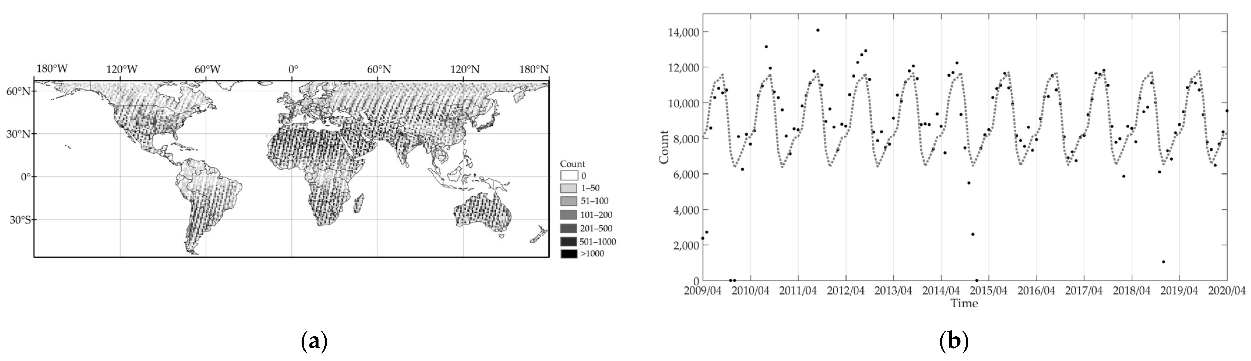
We collected the GOSAT XCH4 retrievals data as Level 2 product (v2.81) released for general users spanning from April 2009 to April 2020, which covers the global land area. We filtered these XCH4 data product using the “quality_flag” tag in the data product documents to get the valid datasets. It has been reported that these XCH4 retrievals have a mean global bias of 1.9 ppb with a standard deviation of 13.4 ppb compared with ground-based observations of the Total Carbon Column Observing Network (TCCON) [32]. Figure 1 shows the density of the collected XCH4 retrieval points from April 2009 to April 2020. As shown in Figure 1, there are many gaps in XCH4 retrievals and the density of data over high latitude and low latitude regions is smaller than that in other regions (Figure 1a). Additionally, the density of retrievals in summer is less than that in winter because of limitations from clear sky conditions and solar zenith angles.
2.1.2. Data for Validation and Analysis
We collected TCCON data and the CH4 simulations from Carbon Tracker-CH4 for the validation of the accuracy of Mapping-XCH4 dataset. Additionally, we collected the surface CH4 emissions data in 2010 from the Emission Database for Global Atmospheric Research (EDGAR).
TCCON, a global network of ground-based Fourier transform spectrometers (FTS) established for the validation of near-infrared total column measurements which has been extensively used for validation of satellite observations [11,33]. The instruments have high accuracy with approximately 0.5% (5 ppb) error in XCH4 retrievals. We collected the available TCCON data released in the 2014 version over 22 sites shown in Figure 1a from 2015 to 2019 to validate the Mapping-XCH4 data.
CarbonTracker-CH4 is released by the National Oceanic and Atmospheric Administration (NOAA). CarbonTracker introduces the assimilation of global atmospheric CH4 observations from surface air samples and tall towers [34,35]. The CarbonTracker-CH4, CT2010, produces estimates of global atmospheric CH4 mole fractions and surface-atmosphere fluxes released from 2000 to 2010. The model-simulated CH4 concentration is gridded CH4 at 4° (latitude) and 6° (longitude) with 25 vertical layers before 2006 and 34 vertical layers after 2006 [36] and with a temporal resolution of 3 h. In comparison with ground-based observations, the model outputs show a mean bias of −10.4 ppb [35]. The CH4 mole fraction profile data from CarbonTracker-CH4 are converted to XCH4 (CT-XCH4) by using the pressure-average method described by Connor et al. [37]. The averaging kernel effect [38] is not considered in the conversion since it has been indicated that the difference is less than 0.1% for XCO2 if averaging kernel smoothing is applied to model simulations or not [39].
To assess the performance of Mapping-XCH4 further, we collected anthropogenic emission data in a 0.1 grid from EDGAR (version 6.0, globally) from 2010 to 2018, which are released by the European Commission’s Joint Research Centre and Netherlands Environmental Assessment Agency [40,41]. EDGAR provides emissions of the three main greenhouse gases (CO2, CH4, and N2O) and fluorinated gases per sector and country. The data are mainly from point source emissions and the global energy statistics database of the International Energy Agency (IEA). The EDGAR CH4 emission data include the emissions from the energy industry, fuel transformation/nonenergy, agriculture, solid waste disposal, fossil fuel fires, large-scale biomass burning, etc. The EDGAR data is a fundamental reference for many studies of surface emissions and have been widely used [42].
2.2. Mapping XCH4 Based on Spatiotemporal Geostatistics
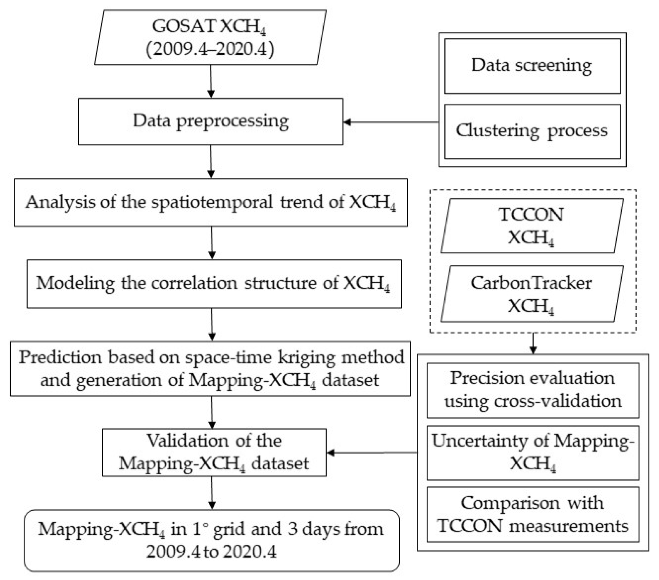
We developed an approach to generate global mapping XCH4 data in a grid of 1° by 1° and intervals of 3 days from 2009 to 2020 by applying spatiotemporal geostatistics to XCH4 retrievals derived from GOSAT observations. Figure 2 shows the main processing steps in the approach, including the analysis of spatiotemporal trend of XCH4, modeling of the correlation structure in space and time, and prediction based on space-time kriging method and generating mapping XCH4. The Mapping-XCH4 data are generated by the optimal prediction of the variable at an unsampled location and time of satellite observation [43,44].
In this study, we only used the XCH4 retrievals with land fractions larger than 90 because the GOSAT retrievals over the ocean from glint mode observations have not been fully validated [45]. We implemented this processing for five mainland subregions in a global land, including Eurasia, Africa, North America, South America, and Oceania. This partition facilitates the processing and geostatistical mapping of XCH4 on a global scale.
2.2.1. Modeling the Spatiotemporal Trend and Correlation Structure of XCH4
XCH4 can be represented by a variable that varies within a spatial domain S and time interval T. Its spatiotemporal variations can be separated into a deterministic trend component and a stochastic residual component , as shown in Equation (1).
Equations (2) and (3).
where , and are the latitude and longitude of the spatial location, respectively. is the marking sequence number of the corresponding time unit, is the background XCH4 at the starting time, and , and are parameters to be estimated by the least-squares technique [26]. As shown in Equation (2), the deterministic spatial trend in , depending on the spatial distribution of CH4 sources and sinks [46], is modeled by a linear surface function [46]. The deterministic temporal trend in , including the interannual XCH4 increase and the inherent seasonal XCH4 cycle, is determined by a set of annual harmonic functions with a simple linear function.
The stochastic residual component in Equation (1), which represents the local variability not explained by the deterministic trend component, is derived by subtracting the trend components from the XCH4 data .
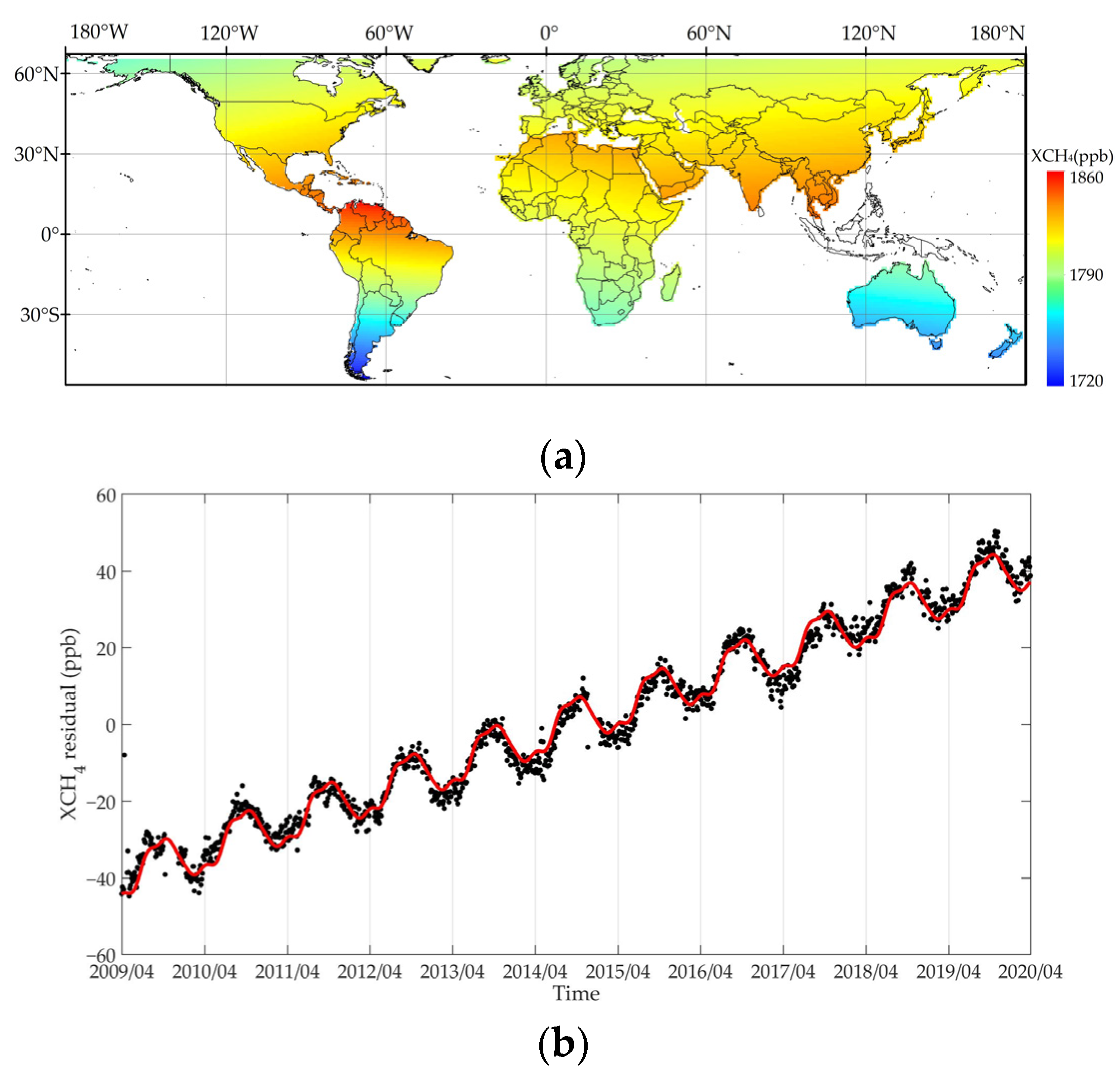
According to the period of GOSAT observation with three days, we set every three days as a time unit, and the annual period is 122 time-units. Figure 3 shows the trend components modeled in space and time. We can find an increasing trend in space from north to south and a temporal trend with a clear annual increase and a seasonal cycle from Figure 3.
In spatiotemporal geostatistical analysis, the optimal kriging prediction of at an unobserved position can be calculated as the linear weighted sum of the XCH4 values that minimizes the mean squared prediction error [22]. The weights for the observations are determined by the distribution of observations and the variogram model, which characterizes the spatiotemporal correlation structure of the data. Therefore, estimating and modeling the variogram are crucial steps in kriging prediction for the global land mapping [46].
The experimental variogram value of XCH4 data at spatial lag and temporal lag is given by:
where is the observation at a spatial location and in a time . is the number of data pairs within a distance of . Once the experimental variogram has been constructed, a spatiotemporal variogram model to fit it. The reason for such a model fit is to make sure the variance model is positive definitive which is required in the calculation of kriging prediction, as is described in Section 2.2.2 below. The spatiotemporal variogram model adopted here is an inseparable combination of the product-sum model [47] and an extra global nugget to capture the nugget effect [48], as given by Equation (4):
where and are the exponential marginal variograms in space and time, respectively, is the fixed spatiotemporal binding parameter to be estimated, and is the global base station value. The admissible value for this is dependent on the sill values of the marginal variograms, namely, . and represent the partial sills of the exponential marginal variograms in space and time, respectively. We used the iterative nonlinear weighted least-square method to estimate all parameters [49].
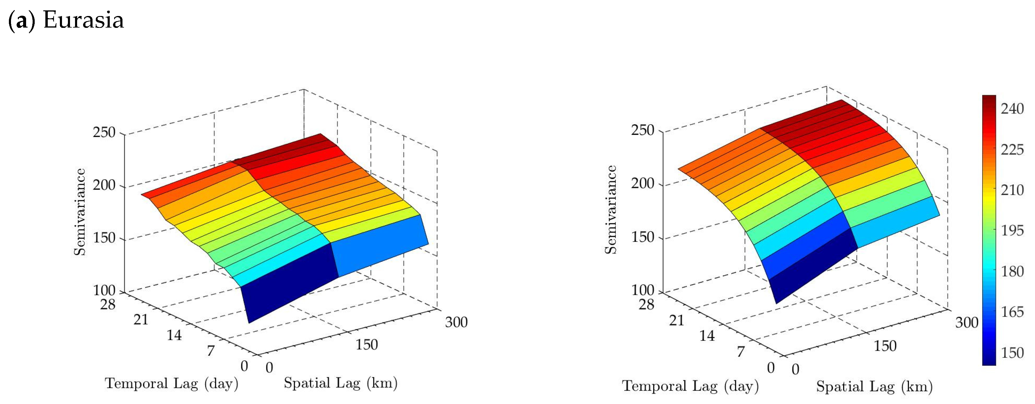
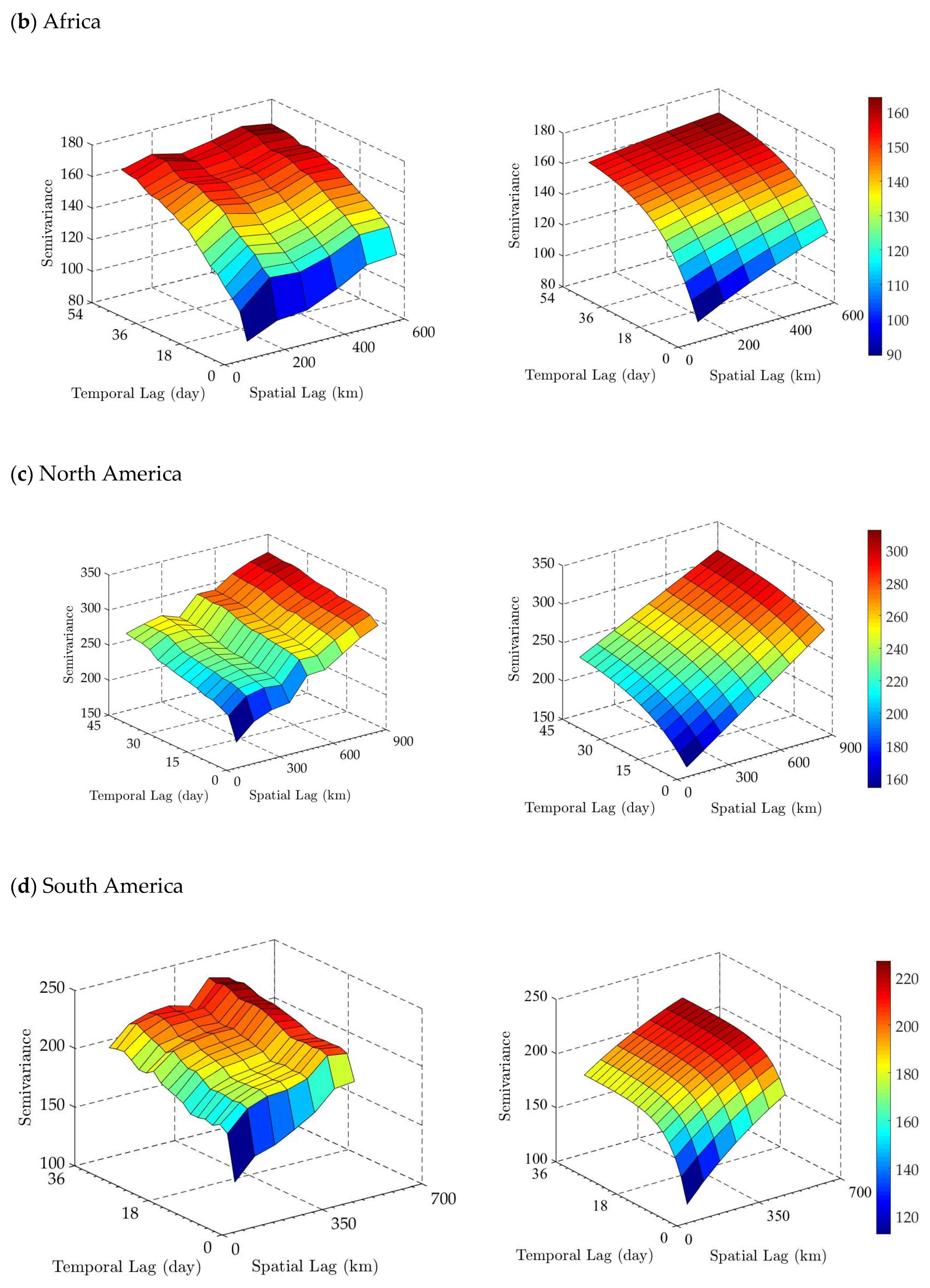
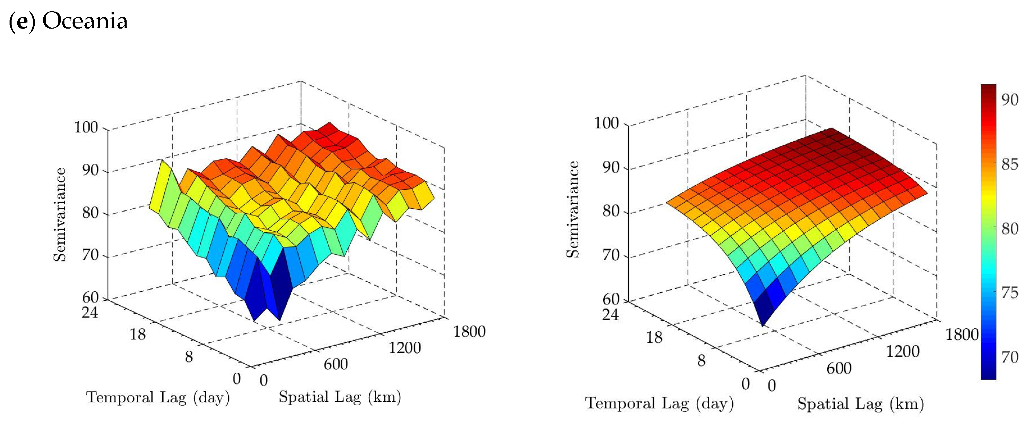
Figure 4 presents the different experimental variogram (left) for the five regions calculated from all GOSAT retrievals by Equation (4) and its fitted variogram model (right) by the product-sum model for five regions. In the variograms shown in Figure 4, the semi-variance values are called nugget and sill when spatial and temporal lag are closet to 0 and infinity, respectively. The ratio of nugget to sill, expressed as a percentage, can be used as an indicator to classify data dependence [50]. In general, a ratio larger than 0.75 indicates a strong spatial or temporal dependence. Table 1 presents the parameters of spatiotemporal variation in five regions. The ratio values of nugget to sill for all regions shown in Table 1 are less than 0.75, which indicates an overall spatial and temporal dependence. The ratio in Eurasia and South America are the lowest which indicates stronger spatial and temporal dependence than the other three regions.
2.2.2. Generating the Mapping-XCH4 Dataset Using Space-Time Kriging
Based on the modeled spatiotemporal variogram, space-time Kriging estimates an arbitrary target point at unobserved location from the stochastic residual component . Supposing that is a prediction of , we estimated as a linear weighted sum of residual data within a kriging neighborhood [22,46] in space and time relative to the prediction location as shown in Equation (5).
where is the number of observations to be used. is the weighting factor assigned to a known observation so as to minimize the prediction error variance while maintaining unbiased prediction. The weighting factor is calculated by Equation (6).
where , is the transpose of matrix, represents the matrix of variogram values between observations, and represents the column vector of variogram values between observations and predictions.
The variance of prediction error, which is a measurement of prediction uncertainty, is shown in Equation (7)
where is the variance of kriging prediction, and 1 is the n × 1 unit vector. The deterministic trend component (the temporal trend of XCH4 as shown in Equation (2) and Figure 3) is tightly constrained since a lot of data available. As indicated by the fitted parameters, the uncertainties are very small compared to the predictive variance in the residual component. Therefore, the uncertainty in the regression mean term is not considered here.
To reduce the computational complexity and maintain local variability, data used in the prediction were searched within an appropriate space-time kriging neighborhood centered on the predicting point [22]. The kriging neighborhood used is a moving cylinder in space and time as described in Zeng et al. [44]. The radii of the search range are initially set to 300 km in space and 20 time-units. The 10 km and 1 time unit for each search process is used as the increment lags if the number of observations is less than 20 within the cylinder neighborhood. At the same time, we set the search range radii limits to 500 km and 40 time-units.
2.3. Precision Evaluation of the Mapping-XCH4 Dataset
We evaluated the performance of the mapping XCH4 dataset using cross-validation and compared it with TCCON measurements and CH4 data simulated by the atmospheric transport model.
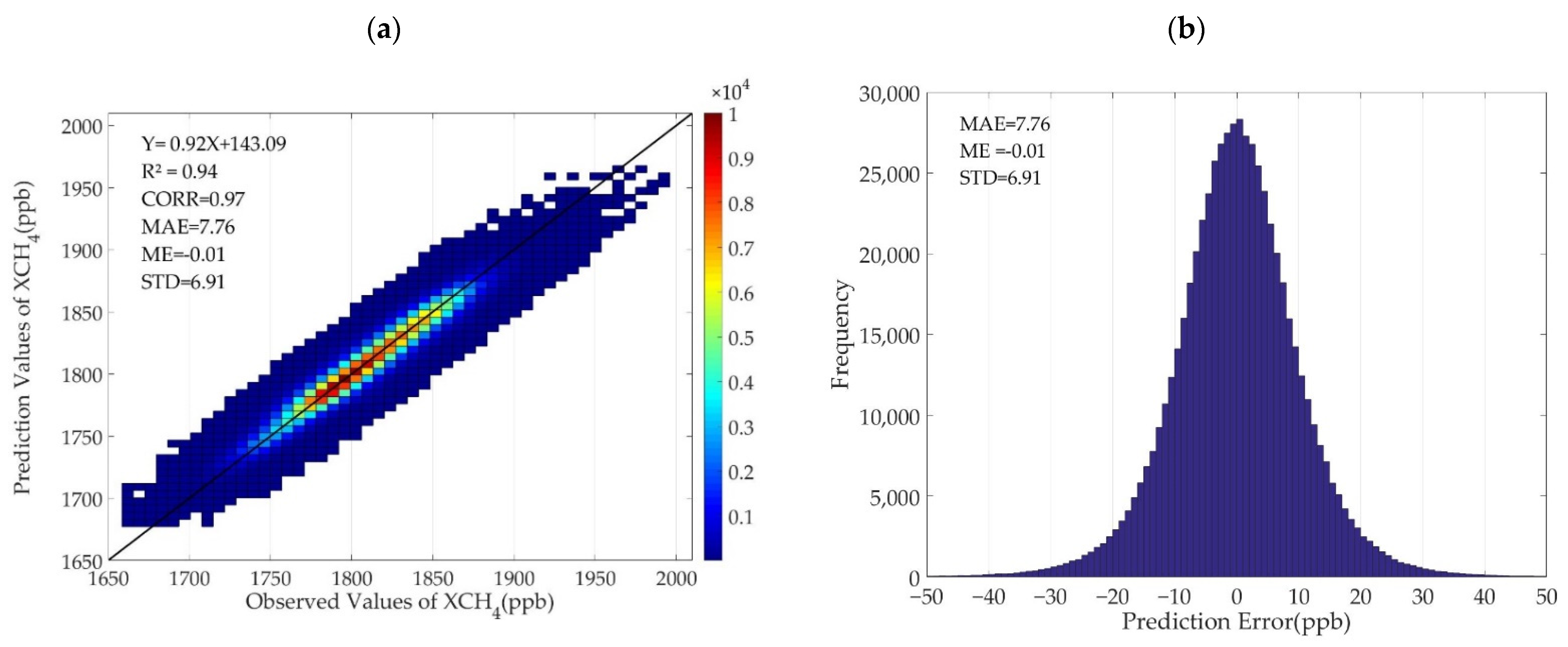
Cross-validation, which is a widely used method for evaluating the prediction accuracy of statistical models [51], can be used to evaluate the prediction accuracy of the spatiotemporal geostatistical method. Cross-validation is implemented by first removing the observation data and then making its prediction using the remaining data. As a result, two datasets, the predicted dataset and the corresponding original dataset , can be obtained. We selected four evaluation criteria, the correlation coefficient (R) between two datasets, the mean absolute prediction error and the percentage of prediction error less than 15 ppb, and the population mean prediction error to evaluate the results [52].
Additionally, we also discussed the performance of the Mapping-XCH4 dataset in detecting the spatial and timely variations from 2009 to 2020 over Monsoon Asia.
3. Evaluation of the Mapping-XCH4 Dataset from 2009 to 2020
3.1. Precision of the Mapping-XCH4 Dataset
3.1.1. Results of Cross-Validation
Figure 5 shows the biases of the predicted values comparing with the corresponding observed values by the cross-validation. The results of cross-validation, as shown in Figure 5, present a significant correlation coefficient (R2) of 0.97 which indicate small prediction biases between the observed XCH4 and the predicted XCH4 data, where the mean MAE is generally 7.76 ppb and the standard deviation (STD) is 6.91 ppb. Figure 5a demonstrates a systematic bias where the observed XCH4 tends to be larger than the predicted XCH4 mostly at high concentrations, while it is smaller than the predicted XCH4 mostly at lower concentrations. This is likely related to the effects of the sensor capability and sensitivity in GOSAT observations for areas with extremely high and low concentrations. The statistical results of cross-validation for the five regions are show in Table 2. It can be seen from Table 2 that the number of predicted data with MAE less than 15 ppb accounts for greater than 83 percent of all validated samples (N). The biases in Eurasia and North America are larger than those in the other regions likely due to the diverse and active surface XCH4 emissions in the two areas.
3.1.2. Uncertainty of Mapping-XCH4
We can obtain the corresponding kriging variance as indicated in Equation (7) for each geostatistical prediction to evaluate the uncertainty of Mapping-XCH4 dataset. The kriging variance depends on both the density of XCH4 retrievals and the data homogeneity surrounding the prediction position. The denser the observations and more homogeneous the XCH4 variation surrounding the prediction position are, the lower the prediction uncertainty [53].
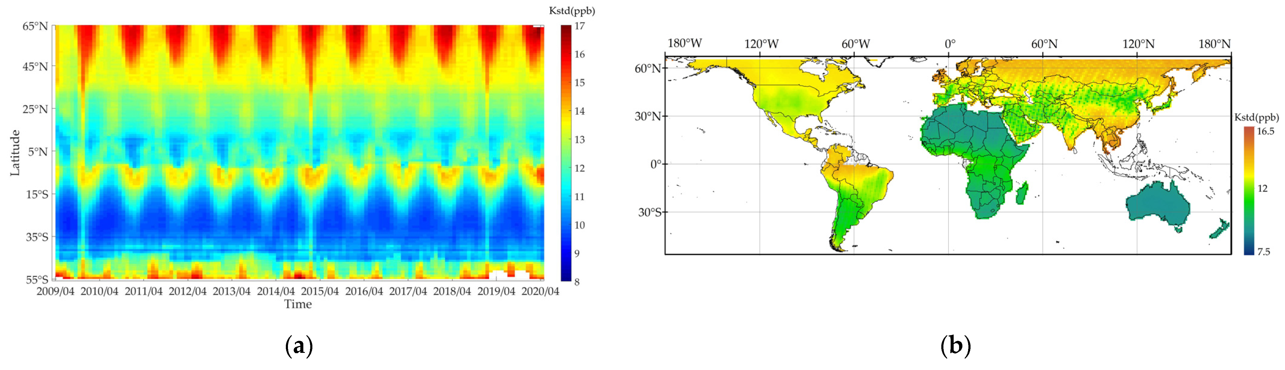
Figure 6a demonstrates the spatiotemporal variation in the kriging standard deviations (Kstd), which is the root of the kriging variance of the Mapping-XCH4 dataset from 2009 to 2020. Figure 6a shows that the uncertainty of Mapping-XCH4 is larger in mid-high latitudes, 35°N–65°N, and around the tropical region, 10°S, where Kstd ranges from 14 ppb to 17 ppb, and seasonally presents a maximum in December or January each year in these areas. In mid-low latitudes, the uncertainty is lower, and Kstd presents a maximum in July or August each year. These high uncertainties are likely due to fewer available observations, which can be seen in Figure 1, less homogeneous variation in XCH4 surrounding the prediction location induced by the effects of atmospheric conditions such as clouds, water vapor, aerosols, etc., and observation of the geometry of the sun-target-sensor geometry.
The magnitude of annual average Kstd, which is shown in Figure 6b, generally presents larger and strip variation in Eurasia compared with the other regions. In particular, Mapping-XCH4 shows higher uncertainties in the southern area of Asia, where Kstd is up to 16 ppb. These results are likely induced by the available GOSAT observations, as shown Figure 1, and inhomogeneous XCH4 variation and atmospheric conditions in these areas.
3.1.3. Comparison with TCCON Measurements
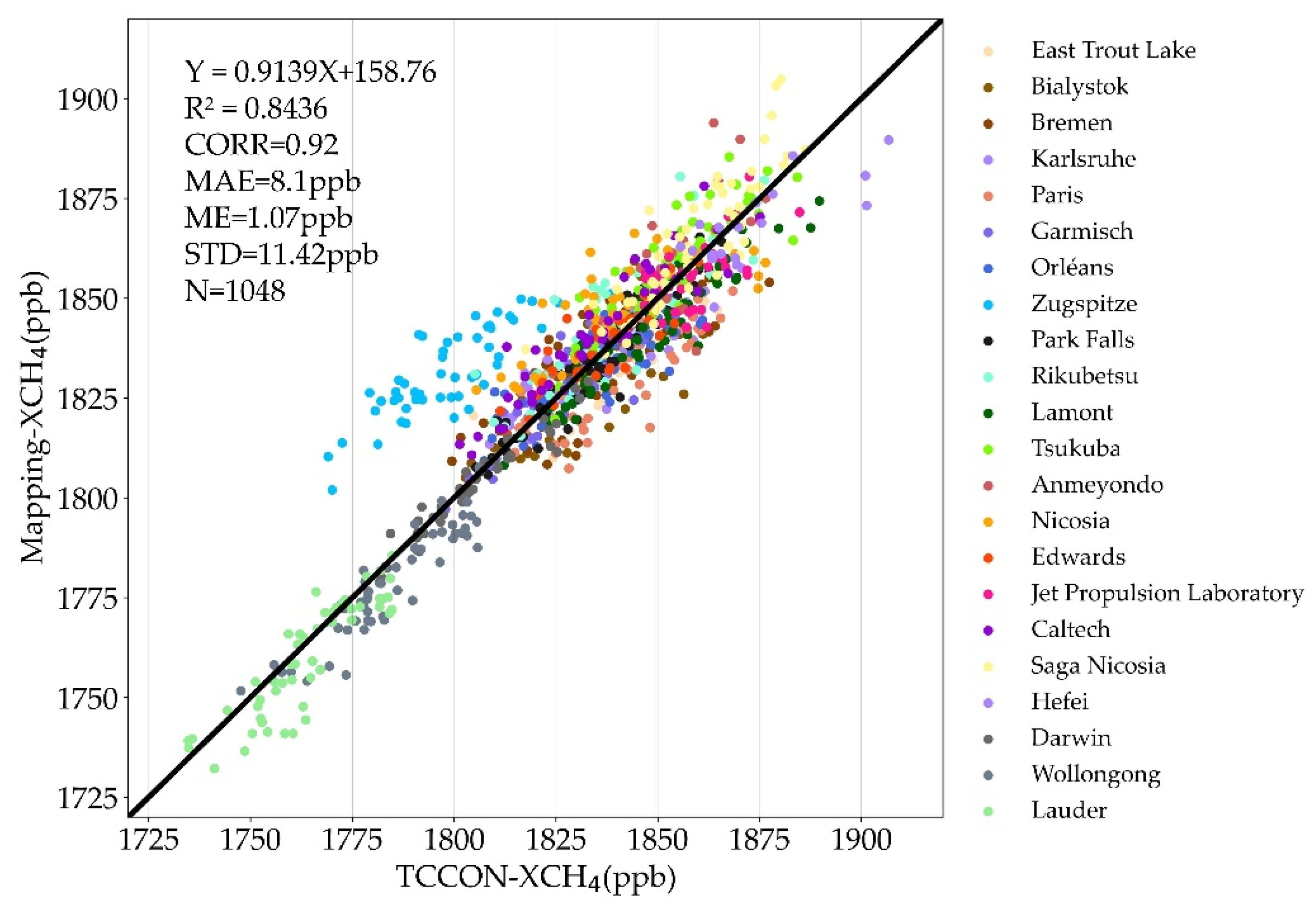
XCH4 from TCCON measurements has high accuracy and can be used for validation of the Mapping-XCH4 [54]. In this study, we selected 22 representative TCCON sites where XCH4 measurements were available from 2015 to 2019. We took 1° × 1° grid and one month as a space-time unit to calculate the mean values of TCCON. Figure 7 shows the biases of Mapping-XCH4 by the comparison of the XCH4 measurements (X-axis) over TCCON sites plotted in different colors and the Mapping-XCH4 (Y-axis) that coincide with TCCON sites in geolocation and time. As seen from Figure 7, the correlation coefficient (CORR), indicating consistency between Mapping-XCH4 and TCCON data, is as high as 0.92, and the mean absolute error (MAE), mean error (ME), and standard deviation (STD) are 8.1 ppb, 1.07 ppb, and 11.42 ppb, respectively.
Overall verification results by TCCON sites (Appendix A Table A1) [55,56,57,58,59,60,61,62,63,64,65,66,67,68,69,70,71,72,73,74,75,76], the MAE is generally 8.10 ppb, while the largest MAEs are over Paris and Zugspitze located in Eurasia, which are 10.61 ppb and 14.60 ppb, respectively. The reasons for these larger biases are likely related to the uncertainty of the Mapping-XCH4 dataset as described above.
3.2. Global XCH4 Variations Revealed by the Mapping-XCH4 Dataset XCH4 in 1° × 1° grids from 2009 to 2020
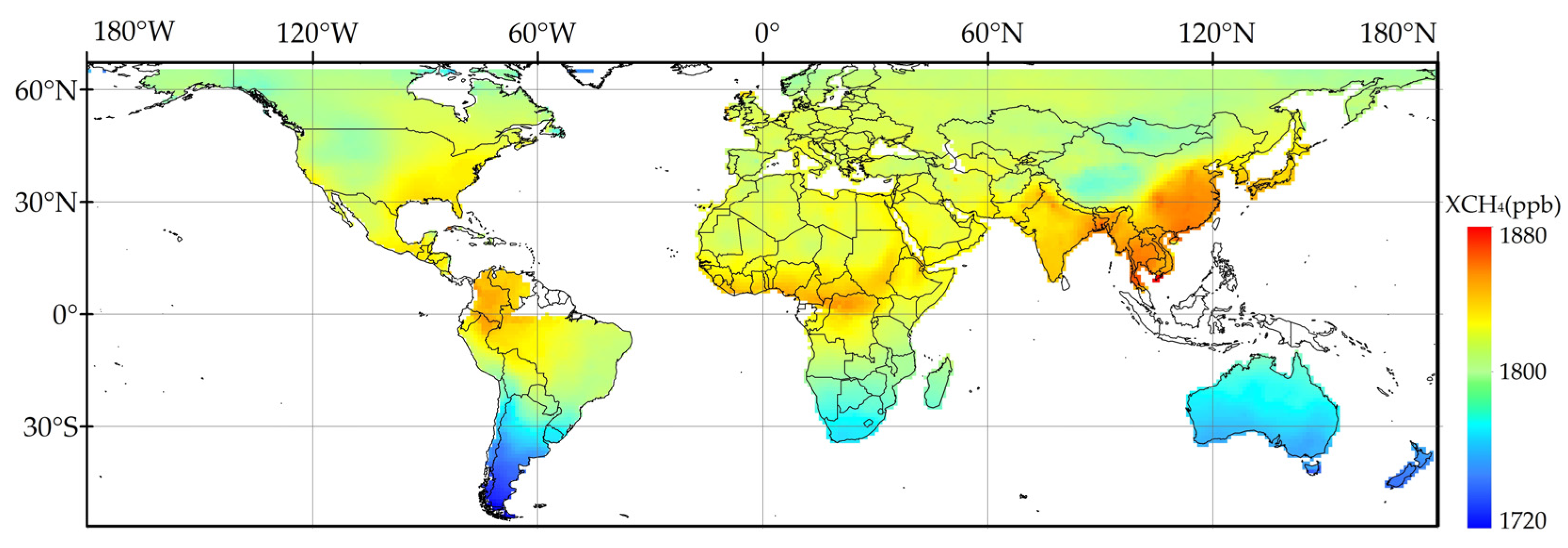
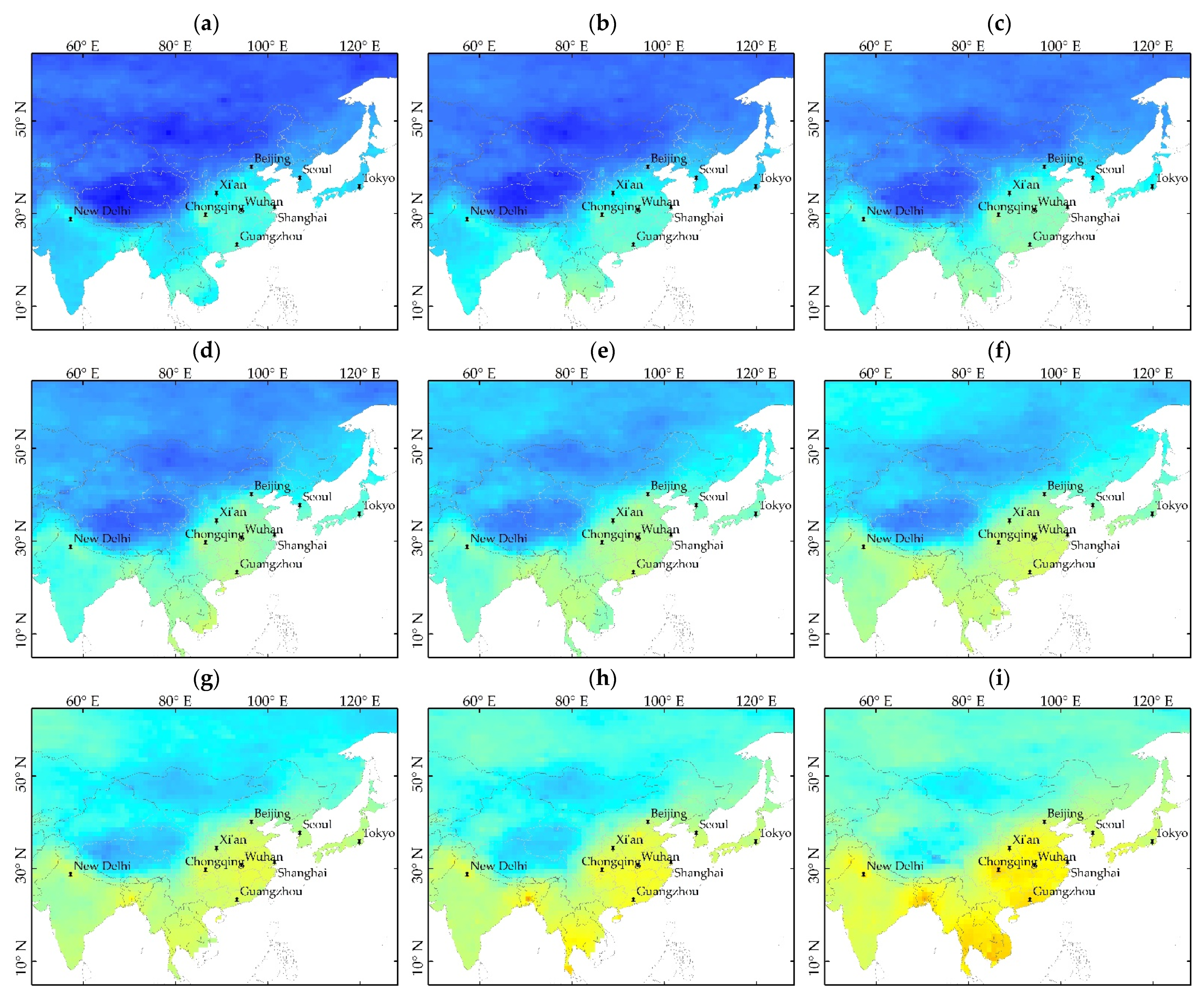
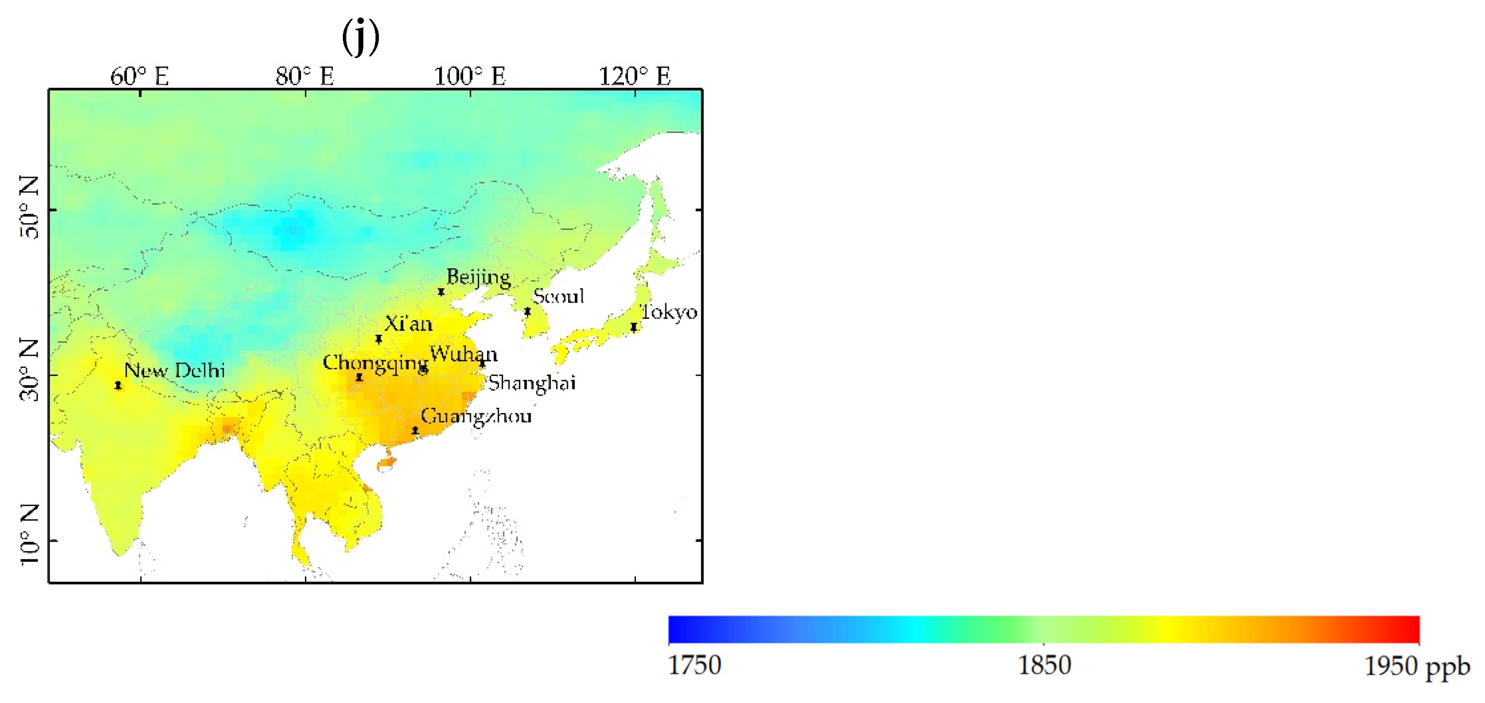
Figure 8 shows the spatial pattern of the annual average XCH4 derived from the Mapping-XCH4 dataset from 2009 to 2020. The local enlarged annual mean Mapping-XCH4 for Monsoon Asia from 2010 to 2020 are shown in Figure A1 in the Appendix A. As shown in Figure 8 and Figure A1 in the Appendix A, the highest XCH4 presents in eastern China and Southeast Asia, which is related to high emissions induced by human activities related to fossil fuel usage and paddy agriculture. It is known that the area of paddy fields in Southeast Asia, including eastern China, accounts for more than 50 percent of the global paddy fields. Spatially, the largest varying amplitude shows in China, where XCH4 generally varies from 1820 ppb to 1860 ppb from the northwest to southeast, and its difference is up to 60 ppb in winter.
The XCH4 around tropical areas in South America and Africa shows higher XCH4 concentrations, which is likely related to wetland emissions. This may also be associated with the uncertainty of Mapping-XCH4 in the tropical area of South America (Figure 6b) caused by much smaller number of available GOSAT XCH4 retrievals (Figure 1a).
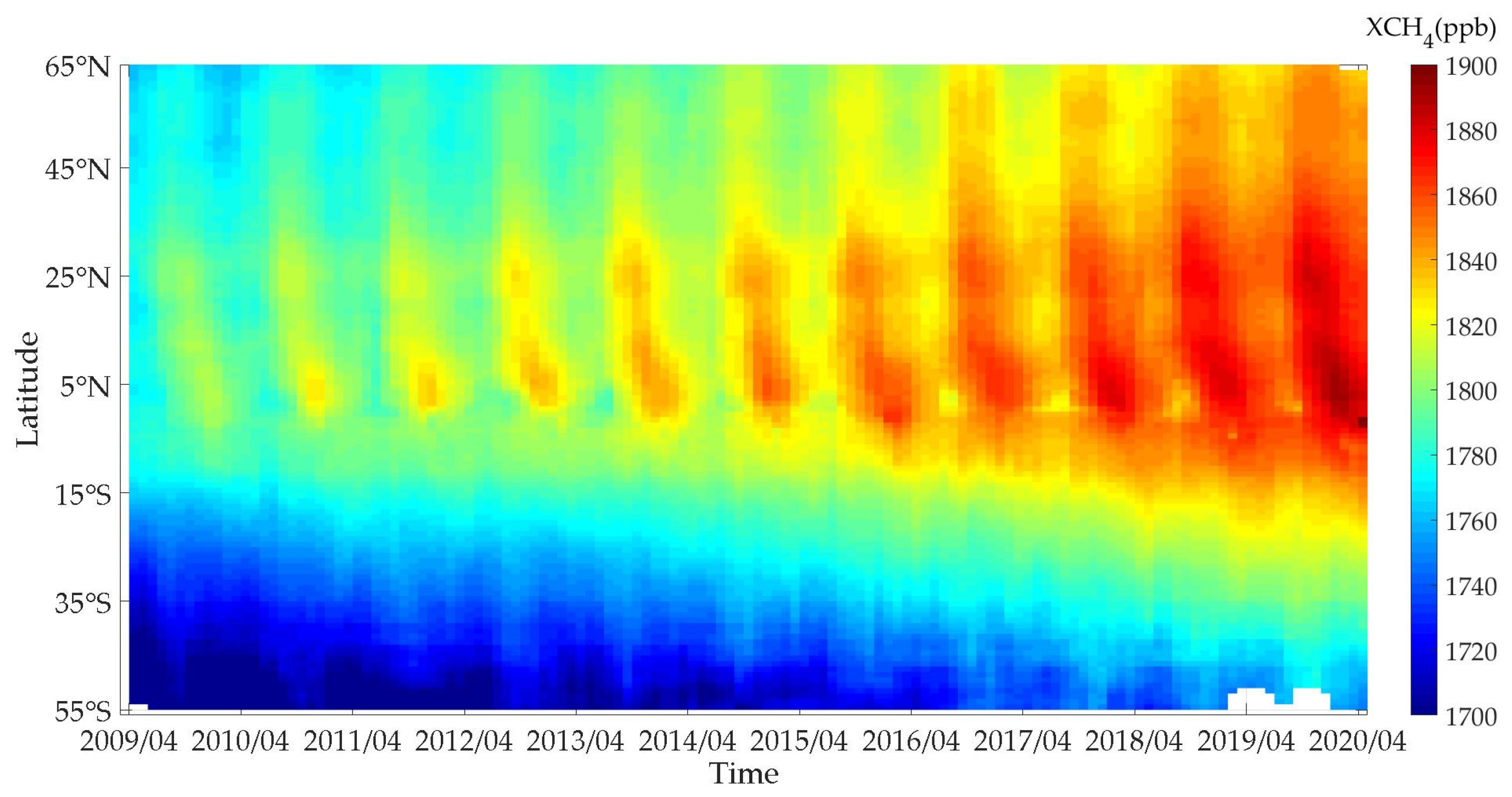
Figure 9 shows the latitudinal and temporal variation in XCH4, which is computed by monthly averaged XCH4 within a 1° latitudinal band using the Mapping-XCH4 dataset in 1° × 1° grids and intervals of three days from April 2009 to April 2020. It can be seen from Figure 9 the Mapping-XCH4 demonstrates an obvious spatial change depending on latitude and a temporally increasing trend in all latitudinal bands. The higher the latitude is, the lower the XCH4 is. Mapping-XCH4 is higher in the Northern Hemisphere than in the Southern Hemisphere due to much higher anthropogenic CH4 emissions in the Northern Hemisphere. High XCH4 values are also present in the equator at approximately 15°N with high temperature and many wetlands, which largely impacts the enhancement of XCH4 surface emissions.
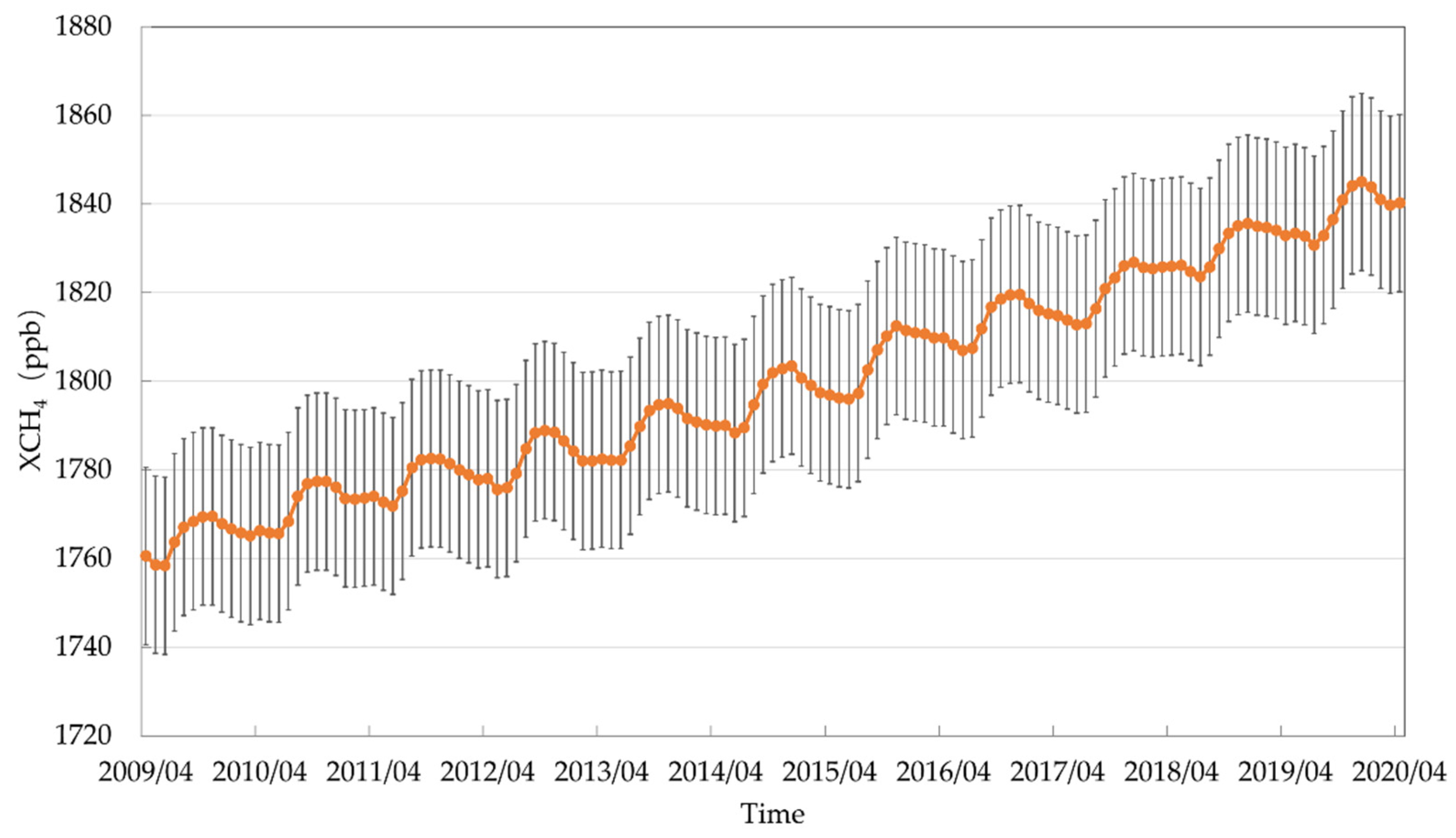
Figure 10 shows the timely variation in globally average XCH4 from 2009 to 2020. The globally average XCH4 presents an annual increase from 2009 to 2020 and seasonal variation which are in agreement with the Global Atmosphere Watch (GAW) report [77]. The maximum XCH4 appeared in November and December, and the minimum appeared in June and July. The seasonal amplitude was up to 11.4 ppb. The seasonal variation in XCH4 is partly driven by the abundance of hydroxyl radicals (OH), the most important sink of CH4, in the atmosphere. As a result, a high abundance of OH in the summer drives down XCH4 [78,79]. Regionally, it could be related to the growth cycle of paddies and vegetation, as well as the change in temperature and humidity caused by the influence of monsoons [80]. Higher temperature and humidity will increase CH4 emissions. Wetlands, such as swamps and lakes, have significant CH4 emissions due to anaerobic environments [80,81].
The mean annual increase in XCH4 was 7.5 ppb/yr during the eleven years from April 2009 to April 2020, which was slightly greater than the mean growth rate of 7.3 ppb/yr during the ten years from Jan 2010 to Dec 2019 reported by the GAW report based on an in situ observational network [77].
3.3. Comparison with Model Simulations of XCH4
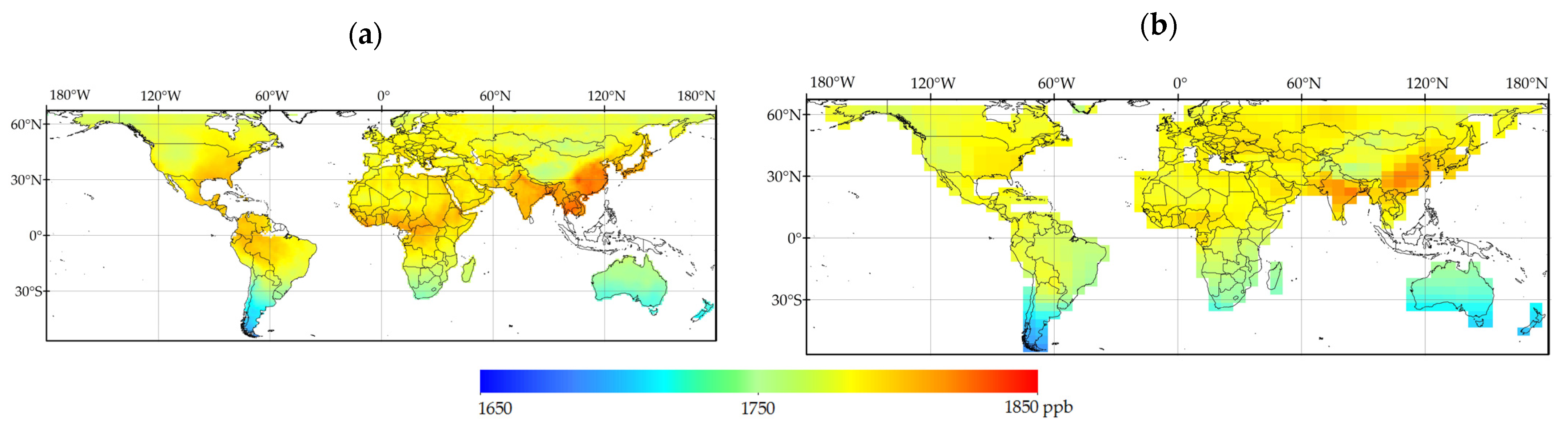
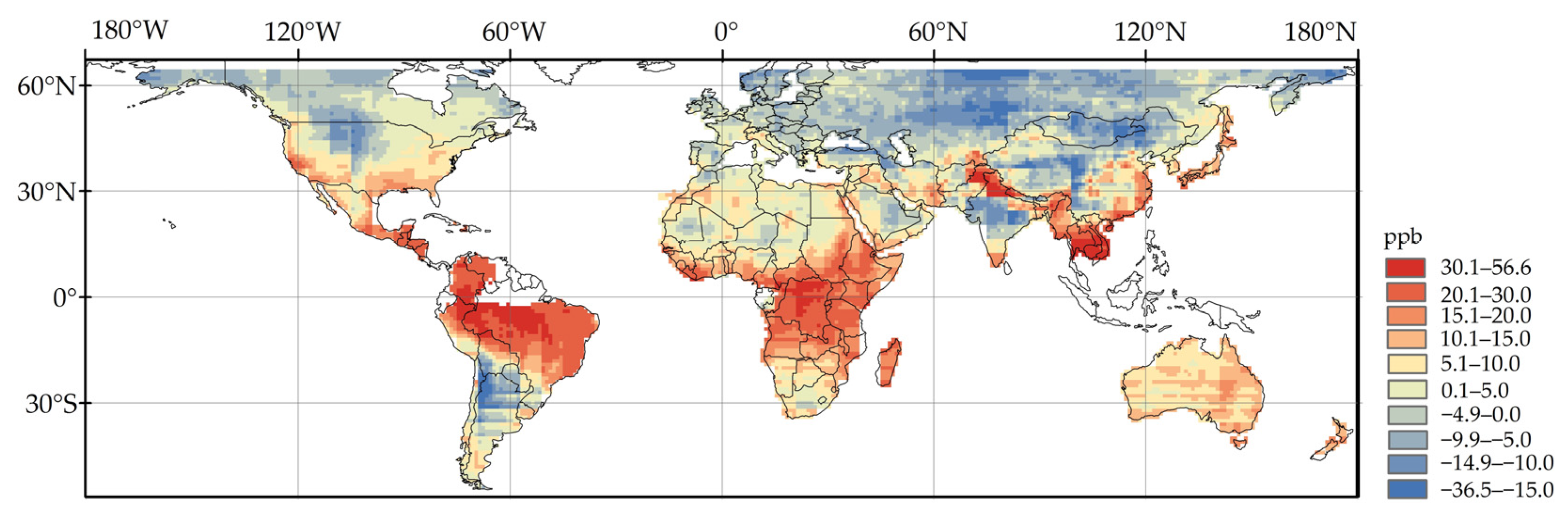
Figure 11 presents the mean XCH4 in 2010 derived from the Mapping-XCH4 dataset and the model simulating XCH4 by CarbonTacker (CT-XCH4) in the same year, and Figure 12 shows their difference. The Mapping-XCH4 generally presents the similar spatial pattern to the CT-XCH4 (Figure 11). The Mapping-XCH4 in Southeast Asia, Northern India and the rainforest in Africa and Southern America, however, are 20–57 ppb larger than the CT-XCH4 as shown in Figure 12. These regions are associated with strong effects of surface emissions, mostly from paddy fields and wetlands in southeastern Asia and tropical areas, and some fossil fuel exploitation and landfills. Mapping-XCH4 in central India, the central area of Northern Asia, North America, and South America is 10–37 ppb smaller than the modeled XCH4.
The large difference in the middle of Africa is likely due to the uncertainty of model simulation in this tropical area rather than the Mapping-XCH4 as the Mapping-XCH4 shows the lowest uncertainties in this area shown in Figure 6b. As a result, the large differences between Mapping-XCH4 and CT-XCH4 mostly arise in the wetland and the paddy fields, which imply that the CT-XCH4 likely have large uncertainty there due to the flaw of prior surface emission in simulating [35].
4. Discussion
4.1. Spatiotemporal Characteristics of Mapping XCH4 Corresponding to the Surface Emissions
The variations in CH4 concentration primarily depend on surface emissions and partly on sinks from chemical reactions in the atmosphere and soil, in addition to atmospheric transport by global and local circulations with seasonality. Surface emissions include anthropogenic emissions from agriculture and waste, fossil fuel production and use, natural emissions from wetlands, geological lakes, termites, biomass burning, etc. The emissions are mostly from agriculture and waste (34%), wetlands (30%), and fossil fuel production and use (19%) [82]. The significantly high correlation between Mapping-XCH4 and the annual surface CH4 emissions in 2010 from the EDGAR emission inventory was shown by Liu et al. [26]. Here, we primarily applied the Mapping-XCH4 dataset from 2009 to 2020 generated by the approach above to reveal the spatiotemporal characteristics of XCH4 corresponding to the surface emissions at the regional scale.
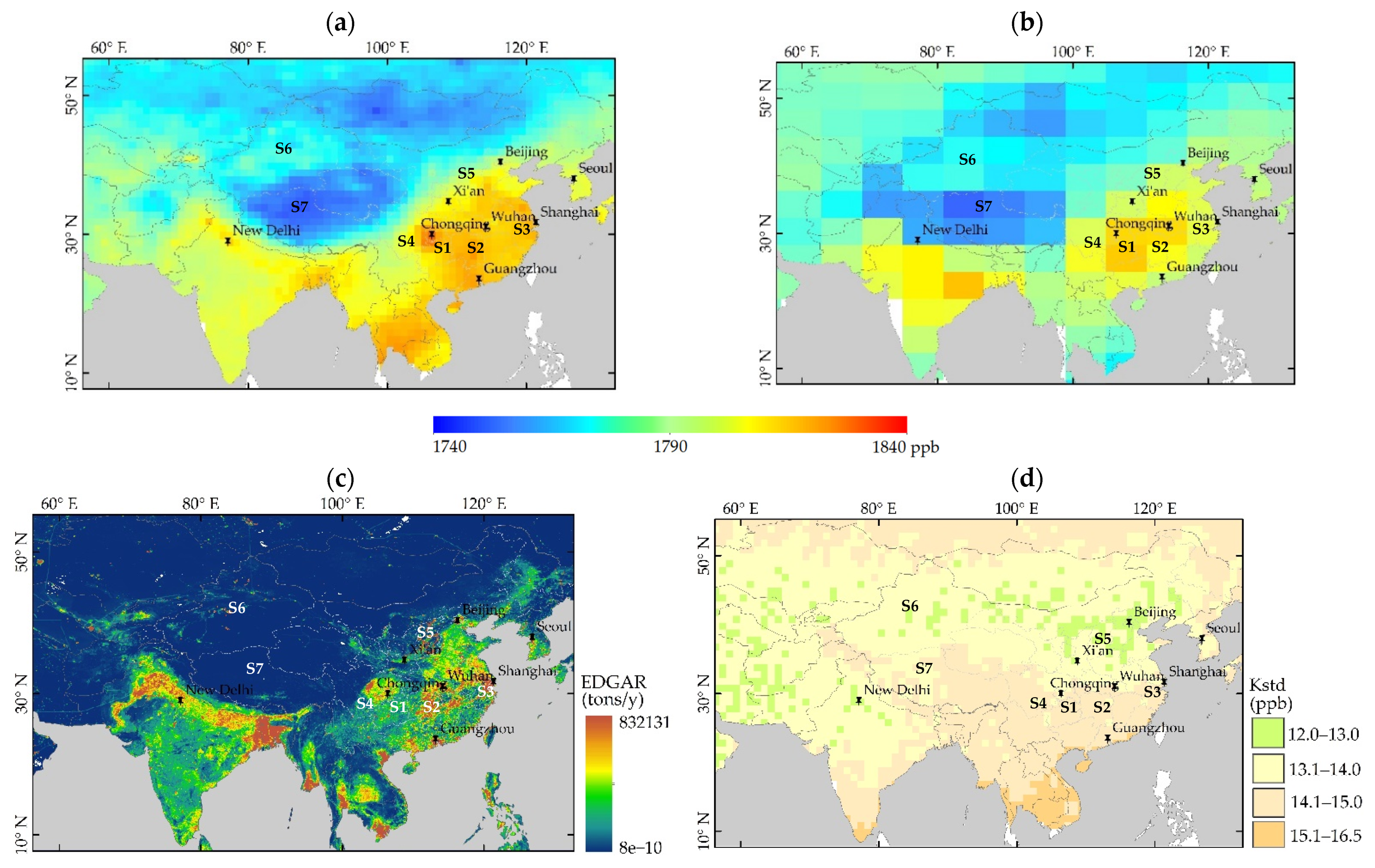
Figure 13 demonstrates the spatial pattern of annual mean XCH4 in 2010 derived from the Mapping-XCH4 and CT-XCH4, respectively, the anthropogenic emissions from EDGAR and the uncertainty (Kstd) of Mapping-XCH4 in the same year. Comparing Mapping-XCH4 with CT-XCH4, as shown in Figure 13a,b, we can find that Mapping-XCH4 reveals a finer spatial variation than CT-XCH4. The spatial pattern of Mapping-XCH4, moreover, is in better agreement with the CH4 emissions of EDGAR (Figure 14) than that of CT-XCH4. In particular, the Sichuan Basin in China, Bangladesh, and northern India with large emissions corresponds to high values in Mapping-XCH4. These large CH4 emissions are mostly related to paddy fields, fossil fuel production and use, and the stagnant effect of the basin terrain [83]. Satellite observations of CO columns and NO2 columns indicated the large magnitude of industrial emissions over this region also [84]. The Mapping-XCH4 does not respond to surface emissions only in the southern tip of the peninsula of South Asia where the large uncertainty of Mapping-XCH4 (Figure 13d) due to a smaller number of available XCH4 retrievals (Figure 1a). These results indicate that the Mapping-XCH4 can reveal and capture the local CH4 emissions in space and time as the Mapping-XCH4 is generated by instantaneous satellite observations that respond to surface emissions [85,86].
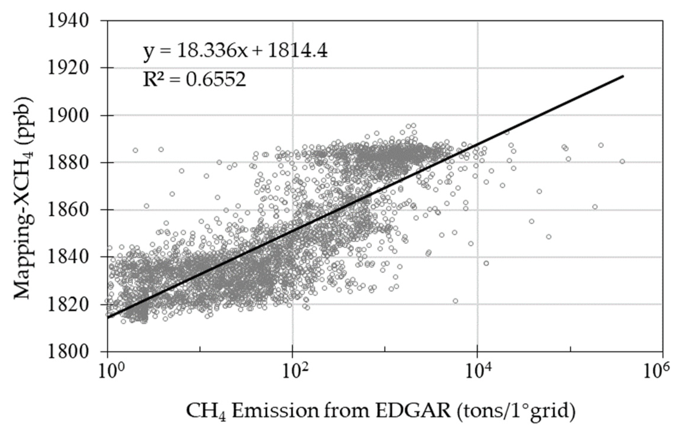
Additionally, Figure 14 shows the correlation between surface emissions and Mapping-XCH4 in Monsoon Asia in 2010. Similarly, a significant linear relationship was also observed by the Mapping-XCH4 data, with a coefficient of determination (R2) of 0.66 and a p value less than 0.01. These results indicated that the variation in CH4 concentration was greatly affected by the surface emissions.
4.2. Temporal Variations of XCH4 for Various Surface Emissions
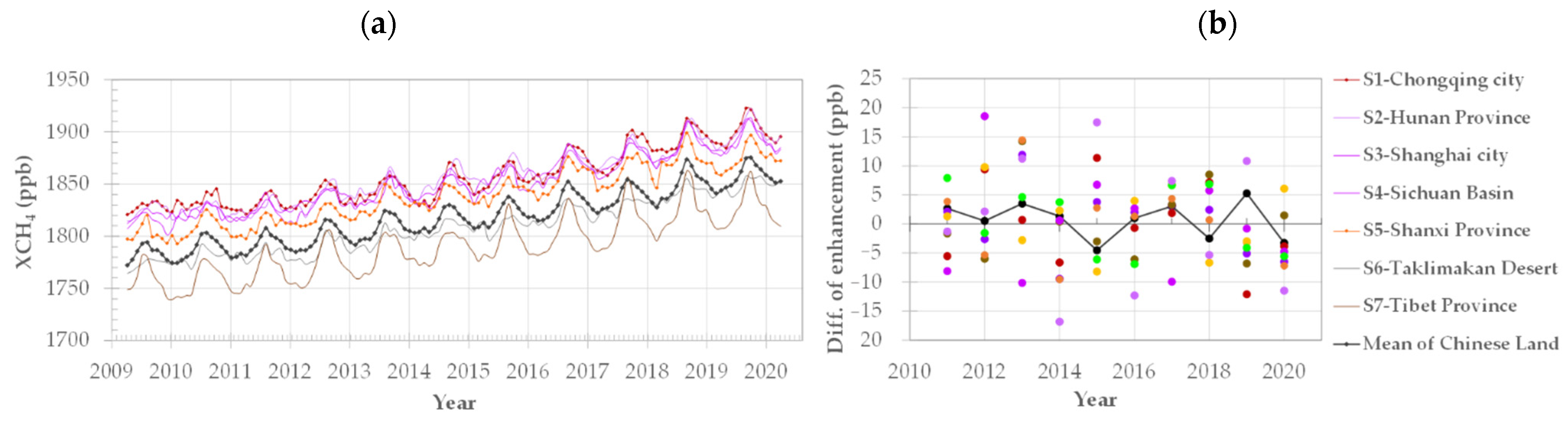
We selected the regions with typical surface emissions which locations are marked as S1–S7 in Figure 13a,c, to investigate the variation of XCH4 revealed by the Mapping-XCH4 datasets. Figure 15 presents a yearly increasing trend from 2009 to 2020 and the difference of annual enhancements for these sampling regions.
It can be seen from Figure 15a that the Tibetan Province (S7) and Taklimakan Deserts (S6) with the lowest emissions (Figure 14), present the minimum XCH4 values of 1790 ± 6.1 ppb and 1808 ± 2.9 ppb, respectively, which are less than the average for all of Chinese land (1818 ± 23.6 ppb). Chongqing (S1), Hunan province (S2), Shanghai city (S3), and the Sichuan Basin (S4) nearly show the highest XCH4, 1858 ± 4.0 ppb, 1857 ± 3.0 ppb, 1853 ± 2.4 ppb, and 1851 ± 8.1 ppb, respectively, which is mostly related to the emissions from the dense oil and gas fields, and paddy fields in addition to the atmospheric accumulation effects due to the geographic basin structure [85]. The XCH4 in Shanxi Province (S5) with high emissions shows the highest standard deviation (9.8 ppb), which is likely induced by many point sources of small or mesoscale coal mines scattered in this region.
The Taklimakan Desert (S6) has the smallest amplitude in seasonal cycle due to less human activity and without vegetation. The Tibetan Province (S7) has the largest amplitude, which is likely induced by the XCH4 emissions from wetlands and meadow grasslands tending to be sensitive to seasonal variations in temperature on the Tibetan Plateau above 4000 m above sea level, the reason of which needs further investigation.
Figure 15b shows the difference of annual enhancement between years during the three months from January to April for the sampling regions. It can be found from Figure 15b that the annual enhancement in 2020 is lower than that in 2019 for the regions except the Shanxi Province (S5) and Taklimakan Deserts (S6), which is likely related with the reduction of anthropogenic emissions caused by the lockdown during this period from January to April in 2020 due to the coronavirus disease 2019 (COVID-19) [87,88]. The NO2 concentration in Shanxi Province during this lockdown period showed the similar change to XCH4 [89], which is likely because the needs of heating in winter did not decrease; thus, there was no significant reduction of emissions from the fossil fuel production and use.
As a result, primarily evaluating the reasonability and potential of the mapping-XCH4 dataset for detecting the variations and the evidence of CH4 above, find (1) the mean annual increase of XCH4 and seasonal variation derived from the Mapping-XCH4 dataset is agreement with that from in-situ observational network; (2) the Mapping-XCH4 dataset could explain the variable of anthropogenic emissions with significant correlation between the Mapping-XCH4 and EDGAR emission inventory (R2 = 0.66) over Monsoon Asia; (3) the Mapping-XCH4 can be used to detect spatiotemporal characteristics regionally, and the evidence of CH4 variations induced by the special events, such as the decrease of XCH4 during January–April in 2020 in China caused by reduction of anthropogenic emission due to the lock down of COVID-19 pandemic.
5. Conclusions
In this study, we proposed a data-driven approach based on a spatiotemporal geostatistical model to generate a global land Mapping-XCH4 dataset in 1° × 1° grids and intervals of 3 days from 2009 to 2020 using XCH4 retrievals derived by GOSAT observations. This Mapping-XCH4 dataset shows better precision with a high correlation coefficient, 0.97, a small mean absolute prediction error of 7.66 ppb in the cross-validation, and good agreement with TCCON sites with a standard deviation of 11.42 ppb. We evaluated the performance of the Mapping-XCH4 dataset by primarily investigating the spatial pattern and timely variation of XCH4 and comparing it with the model simulations. The results show that the timely variations in XCH4 characterized by the Mapping-XCH4 dataset are generally in agreement with the characteristics based on the ground measurements and significantly correlate with the EDGAR emission inventory. The spatial patterns of XCH4 revealed by the Mapping-XCH4 dataset correspond to the distribution of surface CH4 emissions from paddy fields, wetlands, and anthropogenic emissions. Moreover, the Mpping-XCH4 dataset presents a finer spatial pattern than the model simulations. These results demonstrated that the Mapping-XCH4 dataset could help us to investigate the spatiotemporal patterns of XCH4 at global and regional scales. The Mapping-XCH4 dataset has the advantage of being spatiotemporally continuous compared with the original XCH4 retrievals with many gaps in space and time. The Mapping-XCH4 dataset with long-term in grid, such as shown in Figure A1 in Appendix A, facilitates the detection of the driving factors of CH4 variations combined with other satellite observation data, such as ecological parameters of vegetation and land cover related to CH4 natural emissions, and inventory data of agriculture, wetlands, and anthropogenic emissions. This could be like the application of global mapping XCO2 data which are generated by GOSAT observations using geostatistical analysis as well [90,91].
This study assumed that the spatiotemporal correlation structure is similar over the entire processing area. However, this is not always true, as the spatiotemporal variations in different locations are different. The irregular distribution of the original XCH4 retrievals prevents us from resolving this problem. Therefore, the precision of Mapping-XCH4 is mostly due to the number of available GOSAT observations where the more observations there are, the better the geostatistical modeling. Moreover, it also depends on the accuracy of the original XCH4 retrievals derived from satellite observations. Mapping-XCH4 in tropical rainforest areas and high latitudes should receive more attention due to the few observations and limitations of observation conditions there. The uncertainty of Mapping-XCH4 will hopefully be reduced along with increasing XCH4 data available from multiple satellites to improve the geostatistical model.
Author Contributions
L.L. (Luman Li) and L.L. (Liping Lei) conceived and designed the experiments; L.L. (Luman Li) performed the experiments; and H.S. analyzed the data; Z.Z. and Z.H. contributed analytical tools. All authors have read and agreed to the published version of the manuscript.
Funding
This research was funded by the National Key Research and Development Program of China (2020YFA0607503) and the Strategic Priority Research Program of the Chinese Academy of Sciences (XDA19080303).
Acknowledgments
We thank the National Institute for Environment Studies (NIES) for sharing the GOSAT-retrieved XCH4 data products and NOAA ESRL for sharing CarbonTracker-CH4 results. We thank the European Commission Joint Research Centre (JRC) for sharing EDGAR data, which were obtained at https://edgar.jrc.ec.europa.eu/index.php/dataset_ghg60 (accessed on 19 June 2021). The TCCON data were obtained from the TCCON Data Archive hosted by CaltechDATA at https://tccondata.org (accessed on 17 October 2021). We thank TCCON PIs for the TCCON measurements at stations of Anmeyondo, Bialystok, Bremen, Caltech, Darwin, East Trout Lake, Edwards, Garmisch, Hefei, Jet Propulsion Laboratory, Karlsruhe, Lamont, Lauder, Nicosia, Orléans, Paris, Park Falls, Rikubetsu, Saga, Tsukuba, Wollongong, and Zugspitze. The Paris TCCON site has received funding from Sorbonne Université, the French research center CNRS, the French space agency CNES, and Région Île-de-France. The TCCON stations at Rikubetsu are supported in part by the GOSAT series project. Darwin and Wollongong TCCON stations are supported by ARC grants DP160100598, LE0668470, DP140101552, DP110103118 and DP0879468. We thank three anonymous reviewers for their advice on the improvement of the manuscript.
Conflicts of Interest
The authors declare no conflict of interest.
Appendix A

Table A1.
Bias Statistics between the Monthly Average Mapping-XCH4 and TCCON XCH4, which are Calculated as Their Differences for each Coincident Data Pair and Averaged for each Site.
Table A1.
Bias Statistics between the Monthly Average Mapping-XCH4 and TCCON XCH4, which are Calculated as Their Differences for each Coincident Data Pair and Averaged for each Site.
| Sites | Location (Latitude, Longitude) | Coincident Data Pairs | MAE (ppb) | ME (ppb) | Reference |
|---|---|---|---|---|---|
| Lauder | (−45.04°N, 169.68.5°E) | 53 | 5.93 | −3.92 | [55] |
| Wollongong | (−34.41°N, 150.89°E) | 55 | 6.33 | −5.57 | [56] |
| Darwin | (−12.43°N, 130.89°E) | 44 | 3.07 | −1.85 | [57] |
| Hefei | (31.90°N, 117.17°E) | 16 | 7.47 | −4.45 | [58] |
| Saga | (33.24°N, 130.29°E) | 57 | 7.48 | 5.59 | [59] |
| Caltech | (34.14°N, 118.13°E) | 35 | 4.57 | 1.75 | [60] |
| Jet Propulsion Laboratory | (34.20°N, 118.18°E) | 37 | 5.01 | 1.04 | [61] |
| Edwards | (34.96°N, 117.88°E) | 44 | 6.47 | 2.10 | [62] |
| Nicosia | (35.14°N, 33.38°E) | 44 | 7.71 | 3.53 | [63] |
| Tsukuba | (36.05°N, 140.12°E) | 57 | 6.68 | 4.90 | [64] |
| Anmeyondo | (36.54°N, 126.33°E) | 26 | 7.36 | 1.67 | [65] |
| Lamont | (36.60°N, 97.49°E) | 60 | 7.05 | −6.10 | [66] |
| Rikubetsu | (43.46°N, 143.77°E) | 57 | 6.92 | 4.33 | [67] |
| Park Falls | (45.94°N, 90.27°E) | 60 | 4.17 | −0.30 | [68] |
| Zugspitze | (47.42°N, 10.98°E) | 51 | 14.60 | 10.30 | [69] |
| Garmisch | (47.48°N, 11.06°E) | 58 | 4.38 | −0.41 | [70] |
| Orléans | (47.97°N, 2.11°E) | 55 | 6.58 | −1.68 | [71] |
| Paris | (48.85°N, 2.36°E) | 48 | 10.61 | −9.42 | [72] |
| Karlsruhe | (49.1°N, 8.44°E) | 59 | 6.40 | −2.00 | [73] |
| Bremen | (53.1°N, 8.85°E) | 52 | 8.27 | −1.17 | [74] |
| Bialystok | (53.23°N, 23.02°E) | 44 | 7.77 | −3.22 | [75] |
| East Trout Lake | (54.36°N, 104.99°E) | 36 | 6.87 | −4.22 | [76] |
| Overall | - | 1048 | 8.10 | 1.07 | - |
Figure A1.
The annual mean XCH4 in southeastern Asia from 2010 to 2019 is shown in (a)–(j), which are calculated by multitemporal XCH4 data for each year using the Mapping-XCH4 dataset.
Figure A1.
The annual mean XCH4 in southeastern Asia from 2010 to 2019 is shown in (a)–(j), which are calculated by multitemporal XCH4 data for each year using the Mapping-XCH4 dataset.


References
- Wahlen, M. The global methane cycle. Annu. Rev. Earth Planet. Sci. 1993, 21, 407–426. [Google Scholar] [CrossRef]
- Hartmann, D.L. Observations: Atmosphere and surface. In Climate Change 2013: The Physical Science Basis: Contribution of Working GroupI to the Fifth Assessment Report of the Intergovernmental Panel on Climate Change; Cambridge University Press: Cambridge, UK; New York, NY, USA, 2013. [Google Scholar]
- Turner, A.J.; Frankenberg, C.; Kort, E.A. Interpreting contemporary trends in atmospheric methane. Proc. Natl. Acad. Sci. USA 2019, 116, 2805–2813. [Google Scholar] [CrossRef] [PubMed] [Green Version]
- Rigby, M.; Prinn, R.G.; Fraser, P.J.; Simmonds, P.G.; Langenfelds, R.L.; Huang, J.; Cunnold, D.M.; Steele, L.P.; Krummel, P.B.; Weiss, R.F.; et al. Renewed growth of atmospheric methane. Geophys. Res. Lett. 2008, 35, 1–6. [Google Scholar] [CrossRef] [Green Version]
- Dlugokencky, E.J.; Bruhwiler, L.; White, J.W.C.; Emmons, L.K.; Novelli, P.C.; Montzka, S.A.; Masarie, K.A.; Lang, P.M.; Crotwell, A.M.; Miller, J.B.; et al. Observational constraints on recent increases in the atmospheric CH4 burden. Geophys. Res. Lett. 2009, 36, 1–5. [Google Scholar] [CrossRef] [Green Version]
- Nisbet, E.G.; Dlugokencky, E.J.; Bousquet, P. Methane on the rise-again. Science 2014, 343, 493–495. [Google Scholar] [CrossRef] [PubMed] [Green Version]
- Kirschke, S.; Bousquet, P.; Ciais, P.; Saunois, M.; Canadell, J.G.; Dlugokencky, E.J.; Bergamaschi, P.; Bergmann, D.; Blake, D.R.; Bruhwiler, L.; et al. Three decades of global methane sources and sinks. Nat. Geosci. 2013, 6, 813–823. [Google Scholar] [CrossRef]
- Dlugokencky, E.J.; Nisbet, E.G.; Fisher, R.; Lowry, D. Global atmospheric methane: Budget, changes and dangers. Philos. Trans. R. Soc. A 2011, 369, 2058–2072. [Google Scholar] [CrossRef] [PubMed] [Green Version]
- de Gouw, J.A.; Veefkind, J.P.; Roosenbrand, E.; Dix, B.; Lin, J.C.; Landgraf, J.; Levelt, P.F. Daily satellite observations of methane from oil and gas production regions in the United States. Sci. Rep. 2020, 10, 1–10. [Google Scholar] [CrossRef]
- McKain, K.; Wofsy, S.C.; Nehrkorn, T.; Eluszkiewicz, J.; Ehleringer, J.R.; Stephens, B.B. Assessment of ground-based atmospheric observations for verification of greenhouse gas emissions from an urban region. Proc. Natl. Acad. Sci. USA 2012, 109, 8423–8428. [Google Scholar] [CrossRef] [Green Version]
- Wunch, D.; Toon, G.C.; Blavier, J.-F.L.; Washenfelder, R.A.; Notholt, J.; Connor, B.J.; Griffith, D.W.; Sherlock, V.; Wennberg, P.O. The total carbon column observing network. Philos. Trans. R. Soc. A 2011, 369, 2087–2112. [Google Scholar] [CrossRef] [Green Version]
- Butz, A.; Guerlet, S.; Hasekamp, O.; Schepers, D.; Galli, A.; Aben, I.; Frankenberg, C.; Hartmann, J.M.; Tran, H.; Kuze, A.; et al. Toward accurate CO2 and CH4 observations from GOSAT. Geophys. Res. Lett. 2011, 38, 1–6. [Google Scholar] [CrossRef] [Green Version]
- Duren, R.M.; Miller, C.E. Measuring the carbon emissions of megacities. Nat. Clim. Chang. 2012, 2, 560–562. [Google Scholar] [CrossRef]
- Yokota, T.; Yoshida, Y.; Eguchi, N.; Ota, Y.; Tanaka, T.; Watanabe, H.; Maksyutov, S. Global concentrations of CO2 and CH4 retrieved from GOSAT: First preliminary results. Sci. Online Lett. Atmos. Sola 2009, 5, 160–163. [Google Scholar] [CrossRef] [Green Version]
- Bovensmann, H.; Burrows, J.P.; Buchwitz, M.; Frerick, J.; Noël, S.; Rozanov, V.V.; Chance, K.V.; Goede, A.P.H. SCIAMACHY: Mission objectives and measurement modes. J. Atmos. Sci. 1999, 56, 127–150. [Google Scholar] [CrossRef] [Green Version]
- Loyola, D.G.; Gimeno García, S.; Lutz, R.; Argyrouli, A.; Romahn, F.; Spurr, R.J.D.; Pedergnana, M.; Doicu, A.; García, V.M.; Schüssler, O. The operational cloud retrieval algorithms from TROPOMI on board Sentinel-5 Precursor. Atmos. Meas. Tech. 2018, 11, 409–427. [Google Scholar] [CrossRef] [Green Version]
- Wachter, E.D.; Kumps, N.; Vandaele, A.C.; Langerock, B.; Maziere, M.D. Retrieval and validation of MetOp/IASI methane. Atmos. Meas. Tech. 2017, 10, 4623–4638. [Google Scholar] [CrossRef] [Green Version]
- Kuze, A.; Suto, H.; Nakajima, M.; Hamazaki, T. Thermal and near infrared sensor for carbon observation Fourier-transform spectrometer on the Greenhouse Gases Observing Satellite for greenhouse gases monitoring. Appl. Opt. 2009, 48, 6716–6733. [Google Scholar] [CrossRef]
- Tadić, J.M.; Qiu, X.; Yadav, V.; Michalak, A.M. Mapping of satellite Earth observations using moving window block kriging. Geosci. Model Dev. 2015, 8, 3311–3319. [Google Scholar] [CrossRef] [Green Version]
- Yoshida, Y.; Ota, Y.; Eguchi, N.; Kikuchi, N.; Nobuta, K.; Tran, H.; Morino, I.; Yokota, T. Retrieval algorithm for CO2 and CH4 column abundances from short-wavelength infrared spectral observations by the Greenhouse gases observing satellite. Atmos. Meas. Tech. 2011, 4, 717–734. [Google Scholar] [CrossRef] [Green Version]
- Cressie, N.; Wikle, C.K. Statistics for Spatio-Temporal Data; John Wiley & Sons: New York, NY, USA, 2011; pp. 297–360. [Google Scholar]
- Cressie, N. Statistics for Spatial Data; John Wiley & Sons: New York, NY, USA, 1993. [Google Scholar]
- Zeng, Z.C.; Lei, L.P.; Guo, L.J.; Zhang, L.; Zhang, B. Incorporating temporal variability to improve geostatistical analysis of satellite-observed CO2 in China. Chin. Sci. Bull. 2013, 58, 1948–1954. [Google Scholar] [CrossRef] [Green Version]
- Guo, L.J.; Lei, L.P.; Zeng, Z.C.; Zou, P.F.; Liu, D.; Zhang, B. Evaluation of Spatio-Temporal Variogram Models for Mapping XCO2 Using Satellite Observations: A Case Study in China. IEEE J. Sel. Top. Appl. Earth Obs. Remote Sens. 2015, 8, 376–385. [Google Scholar] [CrossRef]
- Katzfuss, M.; Cressie, N. Spatio-temporal smoothing and EM estimation for massive remote sensing data sets. J. Time Ser. Anal. 2011, 32, 430–446. [Google Scholar] [CrossRef]
- Liu, Y.; Wang, X.F.; Guo, M.; Tani, H.S. Mapping the FTS SWIR L2 product of XCO2 and XCH4 data from the GOSAT by the Kriging method-a case study in East Asia. Int. J. Remote Sens. 2011, 33, 3004–3025. [Google Scholar] [CrossRef] [Green Version]
- De Iaco, S.; Posa, D. Predicting spatio-temporal random fields: Some computational aspects. Computers & Geosciences 2012, 41, 12–24. [Google Scholar]
- Finley, A.; Banerjee, S.; Gelfand, A.E. Bayesian dynamic modeling for large space-time datasets using gaussian predictive processes. J. Geogr. Syst. 2012, 14, 29–47. [Google Scholar] [CrossRef]
- Zammit-Mangion, A.; Cressie, N.; Ganesan, A.L.; O’Doherty, S.; Manning, A.J. Spatio-temporal bivariate statistical models for atmospheric trace-gas inversion. Chemom. Intell. Lab. Syst. 2015, 149, 227–241. [Google Scholar] [CrossRef] [Green Version]
- Liu, M.; Lei, L.P.; Liu, D.; Zeng, Z.C. Geostatistical analysis of CH4 columns over Monsoon Asia using five years of GOSAT observations. Remote Sens. 2016, 8, 361. [Google Scholar] [CrossRef] [Green Version]
- Zammit-Mangion, A.; Cressie, N. FRK: An R package for spatial and spatio-temporal prediction with large datasets. J. Stat. Softw. 2021, 98, 1–48. [Google Scholar] [CrossRef]
- NIES GOSAT Project. Summary of the GOSAT Level 2 Data Product Validation Activity; NIES GOSAT Project: Tokyo, Japan, 2019. [Google Scholar]
- Wunch, D.; Toon, G.; Sherlock, V.; Deutscher, N.; Liu, C.; Feist, D.; Wennberg, P. Documentation for the 2014 TCCON Data Release. CaltechDATA. Available online: https://0-doi-org.brum.beds.ac.uk/10.14291/TCCON.GGG2014.DOCUMENTATION.R0/1221662 (accessed on 19 June 2021).
- Peters, W.; Jacobson, A.R.; Sweeney, C.; Andrews, A.E.; Conway, T.H.; Masarie, K.; Miller, J.B.; Bruhwiler, L.; Petron, G.; Hirsch, A.; et al. An atmospheric perspective on North American carbon dioxide exchange: CarbonTracker. Proc. Natl. Acad. Sci. USA 2007, 104, 18925–18930. [Google Scholar] [CrossRef] [Green Version]
- Bruhwiler, L.; Dlugokencky, E.; Masarie, K.; Ishizawa, M.; Andrews, A.; Miller, J.; Sweeney, C.; Tans, P.; Worthy, D. CarbonTracker-CH4: An assimilation system for estimating emissions of atmospheric methane. Atmos. Chem. Phys. 2014, 14, 8269–8293. [Google Scholar] [CrossRef] [Green Version]
- Tsuruta, A.; Aalto, T.; Backman, L.; Hakkarainen, J.; Laanluijkx, I.; Krol, M.C.; Spahni, R.; Houweling, S.; Laine, M.; Dlugokencky, E. Global methane emission estimates for 2000–2012 from CarbonTracker Europe-CH4 v1.0. Geosci. Model Dev. 2017, 10, 1261–1289. [Google Scholar] [CrossRef] [Green Version]
- Connor, B.J.; Boesch, H.; Toon, G.; Sen, B.; Miller, C.; Crisp, D. Orbiting Carbon Observatory: Inverse method and prospective error analysis. J. Geophys. Res. Atmos. 2008, 113, 1–14. [Google Scholar] [CrossRef]
- Rodgers, C.D.; Connor, B.J. Intercomparison of remote sounding instruments. J. Geophys. Res. Atmos. 2003, 108, 1–13. [Google Scholar]
- Cogan, A.J.; Boesch, H.; Parker, R.J.; Feng, L.; Palmer, P.I.; Blavier, J.-F.L.; Deutscher, N.M.; Macatangay, R.; Notholt, J.; Roehl, C.; et al. Atmospheric carbon dioxide retrieved from the Greenhouse gases Observing SATellite (GOSAT): Comparison with ground based TCCON observations and GEOs Chem model calculations. J. Geophys. Res. 2012, 117, 1–17. [Google Scholar] [CrossRef] [Green Version]
- Crippa, M.; Guizzardi, D.; Muntean, M.; Schaaf, E.; Lo Vullo, E.; Solazzo, E.; Monforti-Ferrario, F.; Olivier, J.; Vignati, E. EDGAR v6.0 Global Greenhouse Gas Emissions; European Commission, Joint Research Centre (JRC): Vienna, Austria, 2021. [Google Scholar]
- Crippa, M.; Solazzo, E.; Huang, G.; Guizzardi, D.; Koffi, E.; Muntean, M.; Schieberle, C.; Friedrich, R.; Janssens-Maenhout, G. High resolution temporal profiles in the Emissions Database for Global Atmospheric Research. Sci. Data 2020, 7, 121. [Google Scholar] [CrossRef] [PubMed]
- Baray, S.; Jacob, D.J.; Massakkers, J.D.; Sheng, J.X.; Sulprizio, M.P.; Jones, D.B.; Bloom, A.A.; McLaren, R. Estimating 2010–2015 Anthropogenic and Natural Methane Emissions in Canada using ECCC Surface and GOSAT Satellite Observations. Atmos. Chem. Phys. 2021, 21, 18101–18121. [Google Scholar] [CrossRef]
- He, Z.H.; Lei, L.P.; Zhang, Y.H.; Sheng, M.Y.; Wu, C.J.; Li, L.; Zeng, Z.C.; Welp, L. Spatio-Temporal Mapping of Multi-Satellite Observed Column Atmospheric CO2 Using Precision-Weighted Kriging Method. Remote Sens. 2020, 12, 576. [Google Scholar] [CrossRef] [Green Version]
- Zeng, Z.C.; Lei, L.P.; Hou, S.S.; Ru, F.; Guan, X.H.; Zhang, B. A Regional Gap-Filling Method Based on Spatiotemporal Variogram Model of CO2 Columns. IEEE Trans. Geosci. Remote Sens. 2014, 52, 3594–3603. [Google Scholar] [CrossRef]
- Nguyen, H.; Osterman, G.; Wunch, D.; O’Dell, C.; Castano, R. A method for colocating satellite XCO2 data to ground-based data and its application to ACOS-GOSAT and TCCON. Atmos. Meas. Tech. 2014, 7, 2631–2644. [Google Scholar] [CrossRef] [Green Version]
- Zeng, Z.C.; Lei, L.P.; Strong, K.; Jones, D.B.; Guo, L.; Liu, M.; Deng, F.; Deutscher, N.M.; Dubey, M.K.; Griffith, D.W.T.; et al. Global land mapping of satellite-observed CO2 total columns using spatio-temporal geostatistics. Int. J. Digit. Earth 2017, 10, 426–456. [Google Scholar] [CrossRef] [Green Version]
- De Cesare, L.; Myers, D.E.; Posa, D. Estimating and modeling space-time correlation structures. Stat. Probab. Lett. 2001, 51, 9–14. [Google Scholar] [CrossRef]
- Venetsanou, P.; Anagnostopoulou, C.; Loukas, A.; Lazoglou, G.; Voudouris, K. Minimizing the uncertainties of RCMs climate data by using spatio-temporal geostatistical modeling. Earth Sci. Inform. 2019, 12, 183–196. [Google Scholar]
- Zeng, Z.; Lei, L.; Hou, S.; Li, L. A spatio-temporal interpolation approach for the FTS SWIR product of XCO2 data from GOSAT. IEEE Int. Geosci. Remote Sens. 2012, 852–855. [Google Scholar] [CrossRef]
- Cambardella, C.A.; Moorman, T.B.; Novak, J.M.; Parkin, T.B.; Karlen, D.L.; Turco, R.F.; Konopka, A.E. Field-scale variability of soil properties in lowa Soil. Soil Sci. Soc. Am. J. 1994, 58, 1501–1511. [Google Scholar] [CrossRef]
- Arlot, S.; Celisse, A. A survey of cross-validation procedures for model selection. Stat. Surv. 2010, 4, 40–79. [Google Scholar] [CrossRef]
- Chai, T.; Draxler, R.R. Root mean square error (RMSE) or mean absolute error (MAE)?–Arguments against avoiding RMSE in the literature. Geosci. Model Dev. 2014, 7, 1247–1250. [Google Scholar] [CrossRef] [Green Version]
- Hammerling, D.M.; Michalak, A.M.; Kawa, S.R. Mapping of CO2 at high spatiotemporal resolution using satellite observations: Global distributions from OCO-2. J. Geophys. Res. 2012, 117, 1–10. [Google Scholar] [CrossRef]
- Kivimäki, E.; Lindqvist, H.; Hakkarainen, J.; Laine, M.; Sussmann, R.; Tsuruta, A.; Detmers, R.; Deutscher, N.M.; Dlugokencky, E.J.; Hase, F. Evaluation and analysis of the seasonal cycle and variability of the trend from GOSAT methane retrievals. Remote Sens. 2019, 11, 882. [Google Scholar] [CrossRef] [Green Version]
- Sherlock, V.; Connor, B.; Robinson, J.; Shiona, H.; Smale, D.; Pollard, D. TCCON data from Lauder, New Zealand, 125HR, Release GGG2014R0. 2014. Available online: https://0-doi-org.brum.beds.ac.uk/10.14291/tccon.ggg2014.lauder02.R0/1149298 (accessed on 19 June 2021).
- Griffith, D.W.T.; Velazco, V.A.; Deutscher, N.M.; Paton-Walsh, C.; Jones, N.B.; Wilson, S.R.; Macatangay, R.C.; Kettlewell, G.C.; Buchholz, R.R.; Riggenbach, M. TCCON data from Wollongong (AU), Release GGG2014.R0, TCCON Data Archive, hosted by CaltechDATA. Available online: https://0-doi-org.brum.beds.ac.uk/10.14291/tccon.ggg2014.wollongong01.R0/1149291 (accessed on 19 June 2021).
- Griffith, D.W.T.; Deutscher, N.M.; Velazco, V.A.; Wennberg, P.O.; Yavin, Y.; Keppel-Aleks, G.; Washenfelder, R.; Toon, G.C.; Blavier, J.-F.; Paton-Walsh, C.; et al. TCCON data from Darwin (AU), Release GGG2014.R0, TCCON Data Archive, Hosted by CaltechDATA. Available online: https://0-doi-org.brum.beds.ac.uk/10.14291/tccon.ggg2014.darwin01.R0/1149290 (accessed on 19 June 2021).
- Liu, C.; Wang, W.; Sun, Y.W. TCCON data from Hefei (PRC), Release GGG2014.R0, TCCON Data Archive, Hosted by CaltechDATA. Available online: https://0-doi-org.brum.beds.ac.uk/10.14291/tccon.ggg2014.hefei01.R0 (accessed on 19 June 2021).
- Kawakami, S.; Ohyama, H.; Arai, K.; Okumura, H.; Taura, C.; Fukamachi, T.; Sakashita, M. TCCON data from Saga (JP), Release GGG2014.R0, TCCON Data Archive, Hosted by CaltechDATA. Available online: https://0-doi-org.brum.beds.ac.uk/10.14291/tccon.ggg2014.saga01.R0/1149283 (accessed on 19 June 2021).
- Wennberg, P.O.; Wunch, D.; Roehl, C.M.; Blavier, J.-F.; Toon, G.C.; Allen, N.T. TCCON Data from Caltech (US), Release GGG2014.R1, TCCON Data Archive, Hosted by CaltechDATA. Available online: https://0-doi-org.brum.beds.ac.uk/10.14291/tccon.ggg2014.pasadena01.R1/1182415 (accessed on 19 June 2021).
- Wennberg, P.O.; Roehl, C.; Blavier, J.F.; Wunch, D.; Landeros, J.; Allen, N. TCCON data from Jet Propulsion Laboratory, Pasadena, California, USA, Release GGG2014R0. 2014. Available online: https://0-doi-org.brum.beds.ac.uk/10.14291/tccon.ggg2014.jpl02.R0/1149297 (accessed on 19 June 2021).
- Iraci, L.T.; Podolske, J.; Hillyard, P.W.; Roehl, C.; Wennberg, P.O.; Blavier, J.F.; Allen, N.; Wunch, D.; Osterman, G.; Albertson, R. TCCON Data from Edwards (US), Release GGG2014.R1, Release GGG2014.R1, TCCON Data Archive, Hosted by CaltechDATA. Available online: https://0-doi-org.brum.beds.ac.uk/10.14291/tccon.ggg2014.edwards01.R1/1255068 (accessed on 19 June 2021).
- Petri, C.; Vrekoussis, M.; Rousogenous, C.; Warneke, T.; Sciare, J.; Notholt, J. TCCON Data from Nicosia, Cyprus (CY), Release GGG2014.R0, TCCON Data Archive, Hosted by CaltechDATA. Available online: https://0-doi-org.brum.beds.ac.uk/10.14291/tccon.ggg2014.nicosia01.R0 (accessed on 19 June 2021).
- Morino, I.; Matsuzaki, T.; Horikawa, M. TCCON data from Tsukuba (JP), 125HR, Release GGG2014.R2, TCCON Data Archive, Hosted by CaltechDATA. Available online: https://0-doi-org.brum.beds.ac.uk/10.14291/tccon.ggg2014.tsukuba02.R2 (accessed on 19 June 2021).
- Goo, T.-Y.; Oh, Y.-S.; Velazco, V.A. TCCON data from Anmeyondo (KR), Release GGG2014.R0, TCCON Data Archive, Hosted by CaltechDATA. Available online: https://0-doi-org.brum.beds.ac.uk/10.14291/tccon.ggg2014.anmeyondo01.R0/1149284 (accessed on 19 June 2021).
- Wennberg, P.O.; Wunch, D.; Roehl, C.; Blavier, J.-F.; Toon, G.C.; Allen, N. TCCON data from Lamont (US), Release GGG2014.R1, TCCON Data Archive, Hosted by CaltechDATA. Available online: https://0-doi-org.brum.beds.ac.uk/10.14291/tccon.ggg2014.lamont01.R1/1255070 (accessed on 19 June 2021).
- Morino, I.; Yokozeki, N.; Matsuzaki, T.; Horikawa, M. TCCON data from Rikubetsu (JP), Release GGG2014.R2, TCCON Data Archive, Hosted by CaltechDATA. Available online: https://0-doi-org.brum.beds.ac.uk/10.14291/TCCON.GGG2014.RIKUBETSU01.R2 (accessed on 19 June 2021).
- Wennberg, P.O.; Roehl, C.; Wunch, D.; Toon, G.C.; Blavier, J.-F.; Washenfelder, R.; Keppel-Aleks, G.; Allen, N.; Ayers, J. TCCON Data from Park Falls (US), Release GGG2014.R0, TCCON Data Archive, hosted by CaltechDATA. Available online: https://0-doi-org.brum.beds.ac.uk/10.14291/tccon.ggg2014.parkfalls01.R1 (accessed on 19 June 2021).
- Sussmann, R.; Rettinger, M. TCCON data from Zugspitze (DE), Release GGG2014.R1, TCCON Data Archive, hosted by CaltechDATA. Available online: https://0-doi-org.brum.beds.ac.uk/10.14291/tccon.ggg2014.zugspitze01.R1 (accessed on 19 June 2021).
- Sussmann, R.; Rettinger, M. TCCON data from Garmisch (DE), Release GGG2014.R0, TCCON Data Archive, hosted by CaltechDATA. Available online: https://0-doi-org.brum.beds.ac.uk/10.14291/tccon.ggg2014.garmisch01.R2 (accessed on 19 June 2021).
- Warneke, T.; Messerschmidt, J.; Notholt, J.; Weinzierl, C.; Deutscher, N.M.; Petri, C.; Grupe, P.; Vuillemin, C.; Truong, F.; Schmidt, M.; et al. TCCON data from Orléans (FR), Release GGG2014.R1, TCCON Data Archive, Hosted by CaltechDATA. Available online: https://0-doi-org.brum.beds.ac.uk/10.14291/tccon.ggg2014.orléans01.R1 (accessed on 19 June 2021).
- Te, Y.; Jeseck, P.; Janssen, C. TCCON data from Paris (FR), Release GGG2014.R0, TCCON Data Archive, Hosted by CaltechDATA. Available online: https://0-doi-org.brum.beds.ac.uk/10.14291/tccon.ggg2014.paris01.R0/1149279 (accessed on 19 June 2021).
- Hase, F.; Blumenstock, T.; Dohe, S.; Gross, J.; Kiel, M. TCCON data from Karlsruhe (DE), Release GGG2014.R1, TCCON Data Archive, Hosted by CaltechDATA. Available online: https://0-doi-org.brum.beds.ac.uk/10.14291/tccon.ggg2014.karlsruhe01.R1/1182416 (accessed on 19 June 2021).
- Notholt, J.; Petri, C.; Warneke, T.; Deutscher, N.M.; Buschmann, M.; Weinzierl, C.; Macatangay, R.C.; Grupe, P. TCCON data from Bremen (DE), Release GGG2014.R0, TCCON Data Archive, hosted by CaltechDATA. Available online: https://0-doi-org.brum.beds.ac.uk/10.14291/tccon.ggg2014.bremen01.R1 (accessed on 19 June 2021).
- Deutscher, N.M.; Notholt, J.; Messerschmidt, J.; Weinzierl, C.; Warneke, T.; Petri, C.; Grupe, P.; Katrynski, K. TCCON Data from Bialystok (PL), Release GGG2014.R1, TCCON Data Archive, Hosted by CaltechDATA. Available online: https://0-doi-org.brum.beds.ac.uk/10.14291/tccon.ggg2014.bialystok01.R2 (accessed on 19 June 2021).
- Wunch, D.; Mendonca, J.; Colebatch, O.; Allen, N.T.; Blavier, J.-F.; Roche, S.; Hedelius, J.; Neufeld, G.; Springett, S.; Worthy, D.; et al. TCCON data from East Trout Lake, SK (CA), Release GGG2014.R1, TCCON Data Archive, Hosted by CaltechDATA. Available online: https://0-doi-org.brum.beds.ac.uk/10.14291/tccon.ggg2014.easttroutlake01.R1 (accessed on 19 June 2021).
- WMO (World Meteorological Organization). WMO Greenhouse Gas Bulletin: The State of Greenhouse Gases in the Atmosphere Based on Global Observations through 2019; WMO (World Meteorological Organization): Tokyo, Japan, 2020. [Google Scholar]
- Dlugokencky, E.J.; Steele, L.P.; Lang, P.M.; Masarie, K.A. The growth rate and distribution of atmospheric methane. J. Geophys. Res. 1994, 99, 17021–17043. [Google Scholar] [CrossRef]
- Watson, R.T.; Meira Filho, L.G.; Sanhueza, E.; Janetos, A. Greenhouse gases: Sources and sinks. Clim. Chang. 1992, 92, 25–46. [Google Scholar]
- Thompson, R.L.; Stohl, A.; Zhou, L.X.; Dlugokencky, E.; Fukuyama, Y.; Tohjima, Y.; Kim, S.Y.; Lee, H.; Nisbet, E.G.; Fisher, R.E.; et al. Methane emissions in East Asia for 2000-2011 estimated using an atmospheric Bayesian inversion. J. Geophys. Res. Atmos. 2015, 120, 4352–4359. [Google Scholar] [CrossRef] [Green Version]
- Chandra, N.; Hayashida, S.; Saeki, T.; Patra, P.K. What controls the seasonal cycle of columnar methane observed by GOSAT over different regions in India? Atmos. Chem. Phys. 2017, 17, 12633–12643. [Google Scholar] [CrossRef] [Green Version]
- Friedlingstein, P.; O’sullivan, M.; Jones, M.W.; Andrew, R.M.; Hauck, J.; Olsen, A.; Peters, G.P.; Peters, W.; Pongratz, J.; Sitch, S. Global carbon budget 2020. Earth Syst. Sci. Data 2020, 12, 3269–3340. [Google Scholar] [CrossRef]
- Qin, X.; Lei, L.; He, Z.; Zeng, Z.C.; Matsumi, Y. Preliminary Assessment of Methane Concentration Variation Observed by GOSAT in China. Adv. Meteorol. 2015, 2015, 125059. [Google Scholar] [CrossRef]
- Streets, D.G.; Canty, T.; Carmichael, G.R.; de Foy, B.; Dickerson, R.R.; Duncan, B.N.; Edwards, D.P.; Haynes, J.A.; Henze, D.K.; Houyoux, M.R.; et al. Emissions estimation from satellite retrievals: A review of current capability. Atmos. Environ. 2013, 77, 1011–1042. [Google Scholar] [CrossRef] [Green Version]
- Detmers, R.; Hasekamp, O.; Aben, I.; Houweling, S.; Leeuwen, T.; Butz, A.; Landgraf, J.; Köhler, P.; Guanter, L.; Poulter, B. Anomalous carbon uptake in Australia as seen by GOSAT. Geophys. Res. Lett. 2015, 42, 8177–8184. [Google Scholar] [CrossRef] [Green Version]
- Schneising, O.; Heymann, J.; Buchwitz, M.; Reuter, M.; Burrows, J.P. Anthropogenic carbon dioxide source areas observed from space: Assessment of regional enhancements and trends. Atmos. Chem. Phys. 2012, 12, 31507–31530. [Google Scholar] [CrossRef] [Green Version]
- Stevenson, D.; Derwent, R.; Wild, O.; Collins, W. COVID-19 lockdown NOx emission reductions can explain most of the coincident increase in global atmospheric methane. Atmos. Chem. Phys. Discuss. 2021, 1–8. [Google Scholar] [CrossRef]
- Rajkumar, A.N.; Barnes, J.; Ramachandran, R.; Ramachandran, P.; Upstill-Goddard, R.C. Methane and nitrous oxide fluxes in the polluted Adyar River and estuary, SE India. Mar. Pollut. Bull. 2008, 56, 2043–2051. [Google Scholar] [CrossRef]
- Sheng, M.; Lei, L.; Zeng, Z.; Rao, W.; Zhang, S. Detecting the responses of CO2 column abundances to anthropogenic emissions from satellite observations of GOSAT and OCO-2. Remote Sens. 2021, 13, 3524. [Google Scholar] [CrossRef]
- He, Z.; Zeng, Z.C.; Lei, L.; Bie, N.; Yang, S. A Data-Driven Assessment of Biosphere-Atmosphere Interaction Impact on Seasonal Cycle Patterns of XCO2 Using GOSAT and MODIS Observations. Remote Sens. 2017, 9, 251. [Google Scholar] [CrossRef] [Green Version]
- He, Z.; Lei, L.; Lisa, W.; Zeng, Z.C.; Bie, N.; Yang, S.; Liu, L. Detection of Spatiotemporal Extreme Changes in Atmospheric CO2 Concentration Based on Satellite Observations. Remote Sens. 2018, 10, 839. [Google Scholar] [CrossRef] [Green Version]
Figure 1.
(a) Spatial density of the collected GOSAT XCH4 retrievals in 1° by 1° grid and the locations of TCCON sites used, and (b) temporal variation (gray line) of available GOSAT XCH4 retrieval number (black dots) for each month.
Figure 1.
(a) Spatial density of the collected GOSAT XCH4 retrievals in 1° by 1° grid and the locations of TCCON sites used, and (b) temporal variation (gray line) of available GOSAT XCH4 retrieval number (black dots) for each month.

Figure 2.
The processing flow generating Mapping-XCH4 based on the spatiotemporal geostatistics.

Figure 3.
The trend components derived from eleven years of GOSAT data from April 2009 to April 2020 where (a) is the spatial trend of XCH4, and (b) is the temporal trend (red line) derived by fitting the annual harmonic function and a linear function to the time series of XCH4 residuals (blue dots), which is calculated by averaging the spatially detrended XCH4 data.

Figure 4.
The optimized spatiotemporal experimental variogram of the XCH4 residuals and its fitted variogram model using the product-sum model for five regions: (a–e).
Figure 4.
The optimized spatiotemporal experimental variogram of the XCH4 residuals and its fitted variogram model using the product-sum model for five regions: (a–e).


Figure 5.
(a) Correlation between the predicted values and the corresponding observed values and (b) histogram of the prediction error from cross-validation.
Figure 5.
(a) Correlation between the predicted values and the corresponding observed values and (b) histogram of the prediction error from cross-validation.

Figure 6.
(a) Latitudinal-temporal variability of the uncertainty (Kstd) of predicted XCH4 from 2009 to 2020 with a grid resolution of 1° in latitude and one month in time, (b) the spatial distribution of the annual Kstd of the Mapping-XCH4 dataset from 2009 to 2020.
Figure 6.
(a) Latitudinal-temporal variability of the uncertainty (Kstd) of predicted XCH4 from 2009 to 2020 with a grid resolution of 1° in latitude and one month in time, (b) the spatial distribution of the annual Kstd of the Mapping-XCH4 dataset from 2009 to 2020.

Figure 7.
The relationship between the monthly average values of Mapping-XCH4 (Y-axis) and the XCH4 ground-based measurements (X-axis) over TCCON sites plotted in different colors from 2015 to 2019.
Figure 7.
The relationship between the monthly average values of Mapping-XCH4 (Y-axis) and the XCH4 ground-based measurements (X-axis) over TCCON sites plotted in different colors from 2015 to 2019.

Figure 8.
Spatial distribution of the annual average XCH4 derived from the Mapping-XCH4 data from 2009 to 2020. The blank pixels are the grids where less than five in the eleven-year annual means are available.
Figure 8.
Spatial distribution of the annual average XCH4 derived from the Mapping-XCH4 data from 2009 to 2020. The blank pixels are the grids where less than five in the eleven-year annual means are available.

Figure 9.
Latitudinal-temporal variability of the Mapping-XCH4 dataset from 2009 to 2020 with a grid resolution of 1° in latitude and one month in time.
Figure 9.
Latitudinal-temporal variability of the Mapping-XCH4 dataset from 2009 to 2020 with a grid resolution of 1° in latitude and one month in time.

Figure 10.
Temporal variability in monthly mean XCH4 from April 2009 to April 2020 calculated from Mapping-XCH4 data, where the vertical line in black is the standard deviation of global Mapping-XCH4 data in a month.
Figure 10.
Temporal variability in monthly mean XCH4 from April 2009 to April 2020 calculated from Mapping-XCH4 data, where the vertical line in black is the standard deviation of global Mapping-XCH4 data in a month.

Figure 11.
Spatial distribution of the annual mean in 2010 derived from (a) Mapping-XCH4 data in 1° × 1° grids and (b) the spatial distribution of the CT-XCH4 simulations in 4° × 6° grids.
Figure 11.
Spatial distribution of the annual mean in 2010 derived from (a) Mapping-XCH4 data in 1° × 1° grids and (b) the spatial distribution of the CT-XCH4 simulations in 4° × 6° grids.

Figure 12.
Spatial distribution of annual mean differences between Mapping-XCH4 and CT-XCH4 in 1° × 1° grids in 2010.
Figure 12.
Spatial distribution of annual mean differences between Mapping-XCH4 and CT-XCH4 in 1° × 1° grids in 2010.

Figure 13.
Spatial pattern of annual mean XCH4 in 2010 derived from (a) Mapping-XCH4 and (b) CT-XCH4; (c) anthropogenic emissions from EDGAR in 2010; and (d) the uncertainty (Kstd) of Mapping-XCH4.
Figure 13.
Spatial pattern of annual mean XCH4 in 2010 derived from (a) Mapping-XCH4 and (b) CT-XCH4; (c) anthropogenic emissions from EDGAR in 2010; and (d) the uncertainty (Kstd) of Mapping-XCH4.

Figure 14.
The relationship between CH4 surface emissions and the average XCH4 in 2018 in 1° by 1° grids derived from the Mapping-XCH4 dataset. The black-red line is derived from linear regression of average XCH4 data (Y-axis) and the base 10 logarithm of surface CH4 emissions (X-axis), which shows a significant linear relationship with R2 equal to 0.66 (p value < 0.01).

Figure 15.
The XCH4 variation in the sampling regions: (a) monthly variation of XCH4 from April 2009 to April 2020; (b) the differences of XCH4 yearly enhancement.
Figure 15.
The XCH4 variation in the sampling regions: (a) monthly variation of XCH4 from April 2009 to April 2020; (b) the differences of XCH4 yearly enhancement.

Table 1.
The Parameters of the Spatiotemporal Variogram Model and the Corresponding Nugget/Sill Ratios.
Table 1.
The Parameters of the Spatiotemporal Variogram Model and the Corresponding Nugget/Sill Ratios.
| XCH4 Retrievals | Spatial Lag (km) | Temporal Lag (Days) | Nugget/Sill |
|---|---|---|---|
| Eurasia | 300 | 28 | 0.43 |
| Africa | 600 | 54 | 0.53 |
| North America | 900 | 45 | 0.66 |
| South America | 700 | 36 | 0.43 |
| Oceania | 1800 | 24 | 0.63 |
Table 2.
Results of Cross-Validation for Mapping-XCH4. N is the Number of Validated Sample Pairs.
| Area | N (*104) | R | MAE (ppb) | Percent (MAE < 15 ppb) | ME |
|---|---|---|---|---|---|
| Eurasia | 44.28 | 0.9408 | 8.6319 | 84 | 0.0146 |
| Africa | 40.76 | 0.9636 | 6.9318 | 91 | 0.0021 |
| North America | 13.26 | 0.9314 | 8.8291 | 83 | −0.0072 |
| South America | 13.26 | 0.9604 | 7.7473 | 88 | −0.1034 |
| Oceania | 11.91 | 0.9456 | 6.2717 | 93 | 0.0188 |
Publisher’s Note: MDPI stays neutral with regard to jurisdictional claims in published maps and institutional affiliations. |
© 2022 by the authors. Licensee MDPI, Basel, Switzerland. This article is an open access article distributed under the terms and conditions of the Creative Commons Attribution (CC BY) license (https://creativecommons.org/licenses/by/4.0/).
Share and Cite
MDPI and ACS Style
Li, L.; Lei, L.; Song, H.; Zeng, Z.; He, Z. Spatiotemporal Geostatistical Analysis and Global Mapping of CH4 Columns from GOSAT Observations. Remote Sens. 2022, 14, 654. https://0-doi-org.brum.beds.ac.uk/10.3390/rs14030654
AMA Style
Li L, Lei L, Song H, Zeng Z, He Z. Spatiotemporal Geostatistical Analysis and Global Mapping of CH4 Columns from GOSAT Observations. Remote Sensing. 2022; 14(3):654. https://0-doi-org.brum.beds.ac.uk/10.3390/rs14030654
Chicago/Turabian StyleLi, Luman, Liping Lei, Hao Song, Zhaocheng Zeng, and Zhonghua He. 2022. "Spatiotemporal Geostatistical Analysis and Global Mapping of CH4 Columns from GOSAT Observations" Remote Sensing 14, no. 3: 654. https://0-doi-org.brum.beds.ac.uk/10.3390/rs14030654
Note that from the first issue of 2016, this journal uses article numbers instead of page numbers. See further details here.