Article

Learning-Based Clutter Mitigation with Subspace Projection and Sparse Representation in Holographic Subsurface Radar Imaging

College of Electronic Science and Technology, National University of Defense Technology, Changsha 564211, China
*
Author to whom correspondence should be addressed.
Submission received: 7 December 2021 / Revised: 17 January 2022 / Accepted: 30 January 2022 / Published: 31 January 2022

Abstract

:
The holographic subsurface radar (HSR) is an effective remote sensing modality for surveying shallowly buried objects with high resolution images in plan-view. However, strong reflections from the rough surface and inhomogeneities obscure the detection of stationary targets response. In this paper, a learning-based method is proposed to mitigate the clutter in HSR applications. The proposed method first decomposes the HSR image into raw clutter and target data using an adaptive subspace projection approach. Then, the autoencoder is applied to carry out unsupervised learning to extract the target features and mitigate the clutter. The sparse representation is also combined to further optimize the model and the alternating direction multiplier method (ADMM) is used to solve the optimization problem for precision and efficiency. Experiments using real data were conducted to demonstrate that the proposed method can effectively mitigate the strong clutter with the target preserved. The visual and quantitative results show that the proposed method achieves superior performance on suppressing clutter in HSR images compared with the widely used state-of-the-art clutter mitigation approaches.

1. Introduction

Microwave imaging has been successfully used as a non-destructive remote sensing modality in subsurface targets surveys, including structural assessment [1], landmine detection [2,3,4], and geological exploration [5,6]. Holographic subsurface radar (HSR) is one such technology that uses electromagnetic waves in a frequency band with a narrow width at several discrete frequencies and employs plane scanning of a surface to record subsurface radar holograms with high resolution in plan-view and with low radar cost [7,8]. However, the visibility of shallow buried targets in HSR images is usually obscured by clutter contamination, such as surface reflection, antenna coupling, and the inhomogeneities scattering response [9].
Several techniques were proposed to mitigate the clutter. One simple and convenient method is the mean subtraction (MS) [10]. MS can be regarded as a filter in the time-space domain by averaging the ensemble of radar data and subtracts the mean to reduce the clutter, but this approach will cause distortion to the intensity of target response. Parameter estimation works well when the model parameters are estimated accurately, while how to achieve this estimation is still an open issue [11]. Time gating is an intuitive and simple method to suppress direct coupled waves and ground surface reflection, but application of time gating is prohibited in HSR due to the limited bandwidth and range resolution [12]. The subspace projection methods, such as singular value decomposition (SVD) [13,14,15], principal component analysis (PCA) [16], and independent component analysis (ICA) [17,18], decompose the radar data into several subspaces and remove the clutter subspace for clutter suppression. One issue in subspace projection is the selection of clutter subspace. In [19], morphological component analysis (MCA) is introduced to use different dictionaries to represent clutter morphological component as line-shaped and target morphological component as hyperbola-shaped in radar B-scan images. Its performance depends on the non-adaptive dictionaries that are constructed artificially. Low rank and sparse decomposition (LRSD)-based methods separate the radar data into low rank components, comprising the clutter, and a sparse component, representing the target response [20,21,22,23,24,25]. The clutter and target can be separated by optimizing a low rank and sparse matrix representation problem iteratively.
Recently, learning-based methods were proposed to suppress clutter in subsurface imaging [26,27,28]. In [26], the autoencoders were used to remove the wall interference effects. The main advantage of this technique is that the autoencoders require neither prior information regarding the wall characteristics, nor an analytic model to describe the clutter. The performance of the algorithm is determined by the availability of large training databases of corrupted and clean radar images as well as the hidden layer of the autoencoder. The robust autoencoder (RAE)-based method solves the LRSD problem with the nonlinear representation capability of the autoencoder to catch the low rank components as clutter and achieve better performance than LRSD alone [27]. Another low rank model with an autoencoder was proposed in [28]. This autoencoder has an additional set of parameters to project the input signal to a low rank subspace for clutter mitigation so that the risk of overfitting is reduced and the robustness against noise is improved.
Inspired by the success of low rank and sparse matrix representation and autoencoders for the separation of clutter and target response, this paper proposes a learning-based model with subspace projection and sparse representation for HSR clutter mitigation. Since the clutter in HSR holograms differs from that of radar B-scan images in the difficulties to be formed as the low rank component [29], the initial clutter and target response is decomposed by an adaptive SVD approach [29]. Based on the variance of SVD singular vectors, this approach selects the clutter subspace more accurately and performs better than low rank projection on HSR images. After applying the adaptive SVD, some middle-level clutter can still remain in the initial target images because the real scenes are usually heterogeneous. In this case, the initial target images can be considered noisy. Therefore, instead of large training databases of corrupted and clean radar images in [26], a set of the preprocessed images and their corresponding real target images are used to train the autoencoder, which can reduce the redundant information and risk of overfitting. The real target images are obtained by subtracting the recorded background from the raw radar signals. Then, the trained autoencoder is applied to estimate the target image. Furthermore, we exploit a fidelity term from the estimated target image to inherit the nonlinear representation capability of the autoencoder to capture target response. The optimization model is constituted of the fidelity term, the clutter subspace term, and the joint sparse representation term as well as a set of regularization parameters. Subspace projection and joint sparsity constraint are incorporated to improve the model robustness and reduce the risk of overfitting. The proposed model is solved by the alternating direction method of multipliers (ADMM) [30], and the regularization parameters are estimated using Bayesian optimization [31,32,33,34]. The performance of the proposed method is compared with the commonly used state-of-the-art clutter mitigation algorithms qualitatively and quantitatively.
The rest part of this paper is organized as follows: Section 2 introduces a modified autoencoder model used in this paper, and illustrates the proposed learning-based mitigation method with subspace projection and sparse representation. Section 3 presents the experimental results as well as discussions that demonstrate the effectiveness of our proposed method. Conclusions are drawn in Section 4.

2. Learning-Based Clutter Mitigation for Holographic Subsurface Radar

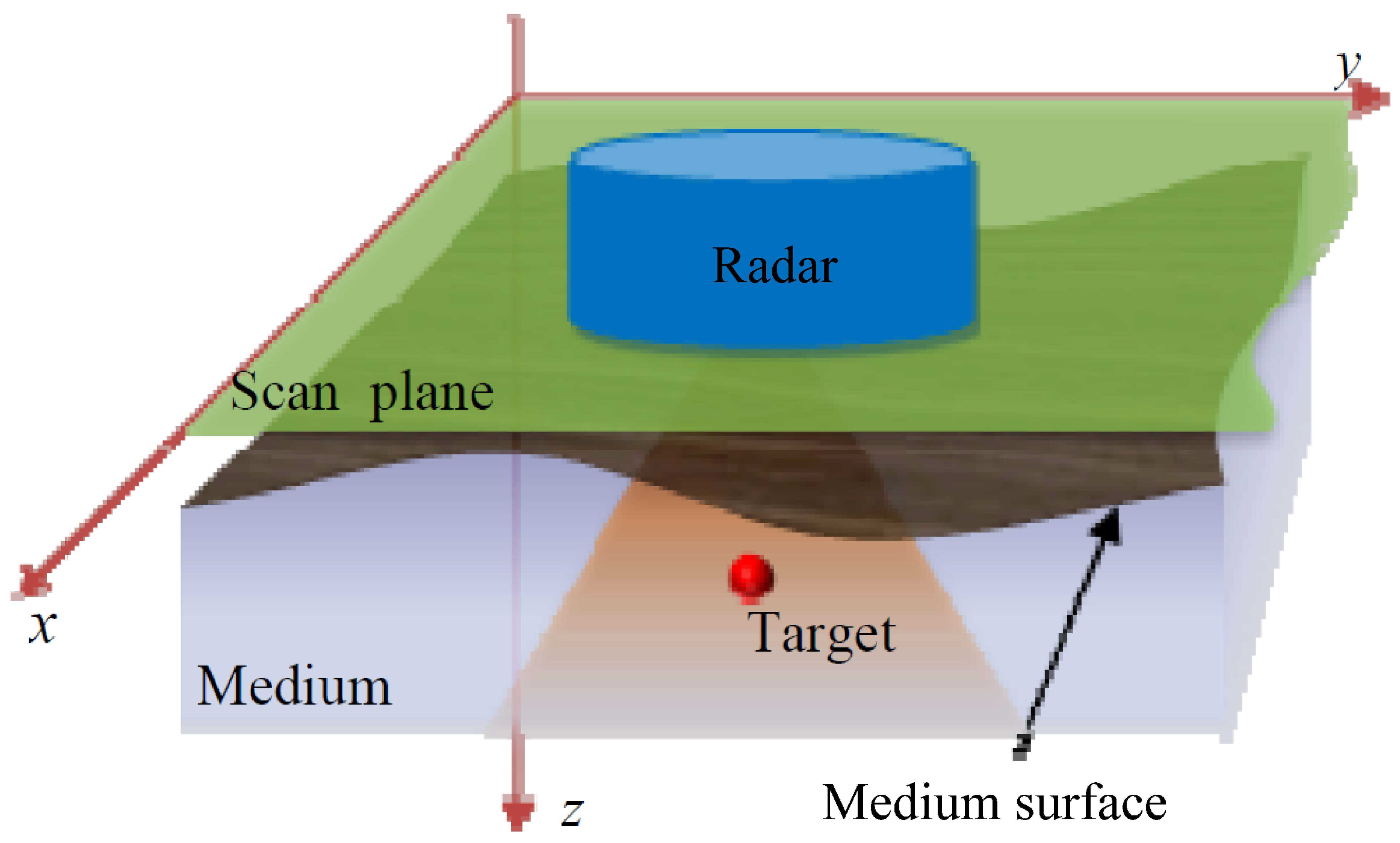
2.1. Holographic Subsurface Radar Model

Unlike GPR B-scan, which is formed along either the cross-track or down-track direction as columns, HSR signals are collected by the radar systems in plan-view scanning of a surface. In this case, each element of the radar echo matrix is an integral of the received signals in the antenna beamwidth at the corresponding scanning location. A simple scenario of HSR imaging through a medium is shown in Figure 1, where a coordinate system is defined to represent the region of interest.
For the simple case of a continuous wave (CW) HSR, the received radar signal at the location ( x , y ) can also be represented as s ( x , y ) . To form a HSR image, the 2-D fast Fourier transform is performed on s ( x , y ) to generate the saliency representation S ( k x , k y ) , where k x and k y denote the wavenumber variables of X and Y directions parallel to scanning plane. Then, a matched filter is imposed on S ( k x , k y ) in the wavenumber domain as
H ( k x , k y ; z ) = j 2 π ( 2 k 0 ) 3 z 3 k z 4 e j k z z
where z denotes the depth in media away from surface, k 0 = 2 π f ε r c denotes the total wavenumber and k z = k 0 2 k x 2 k y 2 denotes the wavenumber variables of Z direction. Finally, the 2-D holographic image can be obtained by implementing the 2-D inverse fast Fourier transform on the results of matched filtering as
I ( x , y ; z ) = IFFT 2 { S ( k x , k y ) × H ( k x , k y ; z ) }
where IFFT2 denotes the 2-D inverse fast Fourier transform. The optimal holographic image can be obtained when the value of z is taken as the actual depth of targets [35,36,37]. In this article, the formed image is a hologram of amplitude and the size is interpolated to 512 × 512 pixels by zero-padding in frequency domain during imaging.
The operating frequency is an important parameter when designing a HSR system, which can be selected according to lateral resolution. For certain transmitting signals, the lateral resolution is related to the accumulated observation angle. Ideally, assume the antennas are omnidirectional and scan along the principal X and Y directions. In this case, the observation angle can reach the range [ π , π ] and the lateral resolution is [7].
δ x = δ y = λ 4
where λ is wavelength of the operating signal.

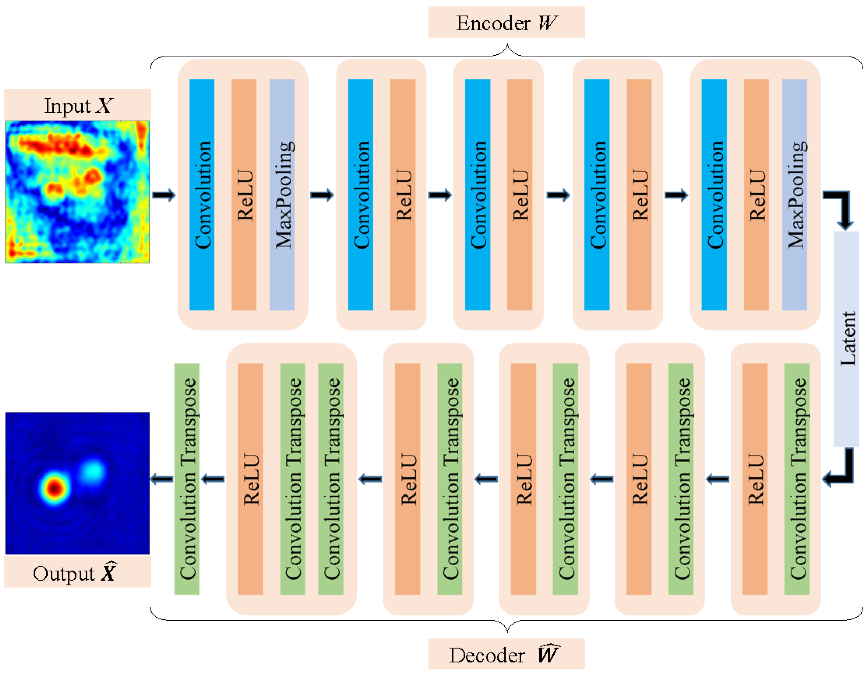
2.2. Theory of Autoencoder

An autoencoder is a type of unsupervised learning artificial neural network that uses an encoder and a decoder to reconstruct the input data. Figure 2 shows the network structure of our autoencoder, used to mitigate clutter. The encoder contains five convolution layers with the kernel of (3, 3), and each convolutional layer is followed by rectified linear unit (ReLU) as the activation function of the convolutional layers which can avoid the phenomenon of gradient vanishing compared to other activation functions (like Sigmoid or tanh). The maxpooling operation is performed with 2 × 2 windows and a stride of 2 to downsample the feature maps after the first and last convolutional layer. The decoder part can be understood as the reverse operation of the encoder to restore the latent vector and ultimately obtain the profile with the same dimensions as the encoder input, therefore completing the denoizing of the images. The input layer and hidden layer form the encoder to compress the high-dimensional input into a low-dimensional latent-space representation. On the other hand, the output layer works as the decoder to reconstruct the input by the inverse mapping from the latent-space representation. Autoencoders have been widely used in data denoizing, dimensionality reduction, and image generation [38,39,40,41,42]. In [26], an autoencoder-based clutter mitigation method was proposed due to the advantage that this technique requires neither prior information regarding the penetrable medium characteristics nor analytic framework to describe the through-medium interference. Instead, the cluttered radar images are considered to be the noisy input and their corresponding target images are treated as clean output. Then, the autoencoder-based algorithm learns how to denoize and clean the corrupted images with training data of clutter and target images.
Mathematically, the training dataset is comprised of K cluttered images { X 1 , X 2 , . . . , X K } i = 1 K and their corresponding clean target images { X 1 t , X 2 t , . . . , X K t } i = 1 K , which are captured by subtracting the background (radar signals collected from the same scene with targets removed) from the raw signals. For the input clutter image X , image denoizing process of the autoencoder can be divided into two steps. In the first step, the encoder tries to learn a compressed latent representation Z of the input X , i.e.,
Z = f ( WX )
where f ( · ) is a nonlinear activation function, and W is the weight matrix of the encoder.
In the second decoder step, an estimated output target image X ^ is reconstructed by the inverse mapping
X ^ = W ^ Z
where W ^ is the weight matrix of the decoder.
Weight matrixes W and W ^ can be optimized during the training stage by minimizing the loss function
min W , W ^ i = 1 K X i t W ^ f ( WX i ) 2 2

2.3. Test of the Standard Autoencoder

For intuitional explanation of the autoencoder performance, two test sets were collected at the Laboratory of Cognitive Radar, National University of Defense Technology, Changsha, China. The stepped-frequency signals, covering a 10–30-GHz frequency band with a step size of 10 MHz, were implemented with the Vector Network Analyzer. The first set (Scene I) was acquired from a scene with a metal circular ring against a concrete slab. Photographs of the measurement setup are depicted in Figure 3. The concrete slab was constructed as a wall with a thickness of 3 cm and relative permittivity (approximately) equals to 6. For the ring target, the radiuses of the inner and outer circle are 2 cm and 4 cm, respectively. The antennas were mounted on a 2D-scanning frame (with a dimension length of 25 cm and width 25 cm with a scanning step of 0.5 cm) and positioned 5 cm above from the slab. All settings of the second scene (Scene II) were the same except that the slab thickness was changed to 5 cm and the measurement geometry can also refer to Figure 3. The autoencoder was trained with a set of 5000 cluttered images and their corresponding target images obtained by background subtraction (80% for training and 20% for validation, the same as in the following article). The training data were recorded of 10 various scenes by our HSR systems, which can record a hologram less than 20 s. In each scene we obtained 500 training images by setting different kinds of targets or targets at different locations with a certain type of of medium such as concrete, planks, bricks, etc.
Figure 4 shows the formed HSR holograms of these two test sets and their corresponding output images obtained with the standard autoencoder, respectively. For quantitative analysis, the Signal to Clutter Ratio (SCR) was adopted to assess the effectiveness of clutter mitigation processing. The SCR can be calculated as
SCR = 10 log ( N c N t p R t I ( p ) 2 p R c I ( p ) 2 )
where I ( p ) is the p-th pixel in the image. N c and N t are the number of pixels in the clutter region R c and target region R t , respectively.
Figure 4a presents the raw holographic image of Scene I obtained at 10 GHz, where the target can be noticed but the clutter is also obvious. Figure 4b shows the image after applying the autoencoder. Comparing Figure 4a,b, we can see the autoencoder-based algorithm effectively removes clutter in the HSR imaging result with a SCR improvement of 11.0 dB. However, in Figure 4c, we can hardly see the target signature since the useful signal suffers extra attenuation through the thicker concrete of Scene II and the surface reflections are dominant in the HSR image. By employing the standard autoencoder, as shown in Figure 4d, the target response is still obscured by the heavy clutter. One reason for the poor performance of the autoencoder in Scene II could be that the target image is totally overlapped by strong clutter, and in this case, the massive redundant information increases the difficulty of extracting target information. It could also be an overfitting problem due to the limited training pairs.
Furthermore, we double the amount of radar data to train the autoencoder. Figure 5a,b shows the formed images of Scene I and Scene II after clutter mitigation by the retrained autoencoder, respectively. Compared to Figure 4b, the target image in Figure 5a is slightly clearer and the SCR is improved by 0.7 dB. The image of the target is still not distinguishable in Figure 5b, which indicates that simply increasing the amount of training data is not the key to improving the performance of standard autoencoder when the target response overlaps with strong clutter.

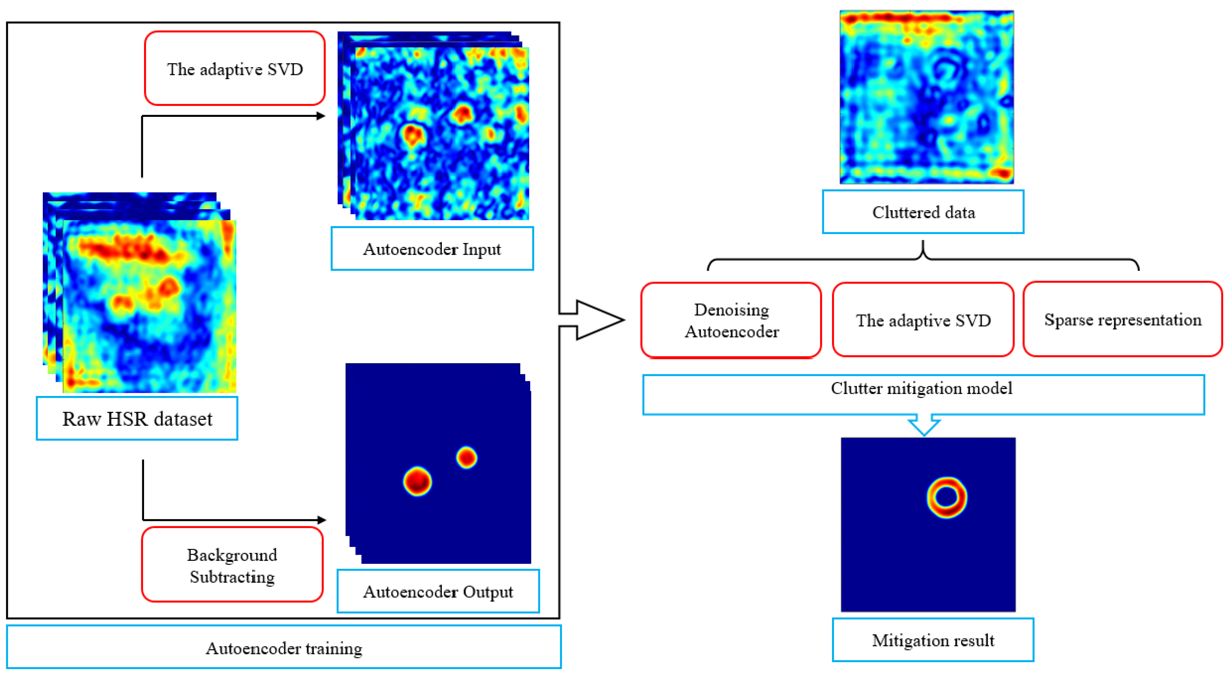
2.4. Denoising Autoencoder for HSR with Subspace Projection

In this section, the adaptive SVD approach is introduced into the autoencoder model [29]. This SVD method concludes that the subspace distribution of target response is related to the variance of left singular vectors based on analysis of the signal cross-correlation characteristics and provides a reliable reference for removing the clutter and extracting the target signal when the obscure barrier is relatively homogeneous. Since the real scene could not be completely homogeneous, a relatively clearer target image with most of the clutter removed is usually obtained after the adaptive SVD. Therefore, the target image with residual clutter can be considered noisy. Then, if we use the target images produced by subspace projection and their corresponding clean target images for training, the clutter mitigation is alleviated by a denoizing process. For the input cluttered image X i , output target image of the denoizing autoencoder model can be written as
X ^ i t = D ( E ( Y i ) )
where X ^ i t is the target image estimated by the denoizing autoencoder, Y i is the target subspace calculated by the adaptive SVD in X i , E ( · ) and D ( · ) represent the encoder and decoder, respectively.
In the modified model, 5000 subspace projection matrixes and their corresponding real target images are similarly applied to train the autoencoder, therefore reducing the redundant information and improving the extraction of salient information. Figure 6a shows the imaging result of Scene II obtained after the adaptive SVD. With calculated clutter subspace removed, the target response is much stronger than that shown in Figure 4c. Figure 6b presents the output image produced by the denoizing autoencoder with subspace projection, which has less clutter than those from standard autoencoder or the adaptive SVD, i.e., in Figure 4d and Figure 6a.

2.5. Learning-Based Clutter Mitigation with Subspace Projection and Sparse Representation

By using the denoizing autoencoder with subspace projection, a clear target image tensor with most of the clutter removed is obtained, yet, there is residual clutter that may raise false alarms. Inspired by the success of Robust Principal Component Analysis (RPCA) in GPR clutter mitigation that separates the clutter and target image by solving a LRSD problem [20], we optimize the autoencoder model to further mitigate the clutter under the RPCA framework.
Mathematically, an observed HSR data matrix X can be decomposed as three components, i.e., the clutter matrix C , the target matrix T and the noise matrix N whose Frobenius norm is assumed to satisfy N F ε for ε > 0 . Thus, the recorded data can be modelled by
X = C + T + N
Since directly extracting the target matrix from the model is a non-convex problem, RPCA treats clutter as a low-rank matrix and targets as a sparse matrix based on LRSD theory. Then Equation (9) can be rewritten as
X = L + S + N
where L R M × N and S R M × N correspond to the low-rank clutter and sparse target parts, respectively, thus the problem in Equation (10) can be solved by following convex optimization [21].
min L , S L * + λ S 1 s . t . X L S F ε
where · * denotes the nuclear norm used to sum singular values of the matrix, · 1 denotes the l 1 norm which calculates the sum of the absolute values of the matrix entries, and λ is a positive regularization parameter that controls the sparsity of the sparse matrix S . Under certain noise sparsity and rank upper-bound assumptions, the low-rank clutter matrix L and sparse target matrix S can be recovered.
However, the performance of RPCA on HSR images is not so good as that on radar B-scan images due to the difficulty for appropriate low-rank matrixes to represent clutter in such plan-view holograms where clutter distributes homogeneously [29]. Therefore, the proposed method catches the sparse target component in a similar way to RPCA, i.e., by the l 1 norm, but inherits the subspace selection capability of the adaptive SVD to suppress the strong HSR clutter. In addition, by combining the denoizing autoencoder terms, the clutter mitigation model can be reformulated as a constrained optimization problem
min C , T 1 2 T D ( E ( Y ) ) F 2 + α C * + β T 1 s . t . X C T F ε
where Y is the initial target estimated by the adaptive SVD, and α and β are the regularization parameters. The first item of model is used to constrain that the calculated target matrix approximates the result of the autoencoder. Instead of setting the initial parameter values to zero by RPCA, the proposed model applies clutter and target matrixes obtained by the adaptive SVD as initial values to iterate, therefore improving the extracting of salient information for more optimal solutions.
The constrained problem Equation (12) can be addressed by the following augmented Lagrangian function [30].
L ( C , T , Z ) = 1 2 T D ( E ( Y ) ) F 2 + α C * + β T 1 + Z H ( X C T ) + μ 2 X C T F 2
where Z denotes the Lagrangian multiplier and μ > 0 is a penalty parameter. Then the variables C , T , and Z can be solved by the ADMM algorithm which updates each variable alternately by minimizing the augmented Lagrangian function with other variables fixed. Therefore, (13) is decomposed as following subproblems.
C k + 1 = arg min C α C * + μ 2 X C T k + Z k μ F 2
T k + 1 = arg min C 1 2 T D ( E ( Y ) ) F 2 + β T 1 + μ 2 X C k + 1 T + Z k μ F 2
Z k + 1 = Z k + μ ( X C k + 1 T k + 1 )
Since subproblem (14) is a least-squares problem regularized by a nuclear norm penalty, it can be solved by singular value shrinkage [30]. The shrinkage operator T ( a , b ) is defined as follows
T ( a , b ) = a b a > b 0 a b a + b a < b
Then we can update C k + 1 by applying the singular value thresholding [43].
SVD ( X T k + Z k μ ) = U Σ V T
C k + 1 = U T ( Σ , α μ ) V T
where U and V are unitary matrixes, and Σ is a diagonal matrix of singular values.
Subproblem (15) can be rewritten after some algebraic manipulations as
T k + 1 = arg min C β T 1 + μ 2 μ μ + 1 ( X C k + 1 + Z k + D ( E ( Y ) ) μ ) T F 2 + C
where C is a constant term independent of T . To solve the squares problem regularized by the l 1 norm, we can use the shrinkage operator as
T k + 1 = T ( μ μ + 1 ( X C k + 1 + Z k + D ( E ( Y ) ) μ ) , β μ )
Suppose the size of an acquired holographic image is M × N ( M N ) , the solving procedures are summarized in Algorithm 1. The proposed clutter mitigation algorithm estimates the clutter and target matrix by solving several subproblems, which have an overall computational complexity of O ( M 3 + N 2 + N 3 ) for each iteration. Even though the proposed model is slightly more computationally expensive than RPCA, which has an overall computational complexity of O ( M N 2 ) for each iteration, it is much more efficient than MCA which has an extra requirement for appropriate dictionaries. Considering an image of size 512 × 512 , the running-time of RPCA, MCA and the proposed algorithm in the same platform are 1.8 s, 291.4 s and 4.1 s, respectively.
The structure of the proposed method is shown in Figure 7. First, the raw dataset of various scenes mentioned above is acquired by our radar system. Then, the input and out datasets are obtained for supervised training by applying the adaptive SVD and background subtracting to the raw dataset. The autoencoder can learn how to denoize or clean the cluttered images using training data comprising both cluttered and clean data. After training the denoizing autoencoder, the proposed clutter mitigation model is performed by minimizing a constrained optimization problem with the adaptive SVD and joint sparsity constraints. Finally, a test image out of the training set is employed to evaluate the performance of the model.
Algorithm 1:The ADMM for the learning-based model with subspace projection and sparse representation
Input: X , Z 0 = 0 , T 0 = Y , C 0 = X Y , α , β , μ = 0.25 i = 1 M j = 1 N | X ( i , j ) | / M N ,
     K = 50 , ε = 1 e 6
Output: C, T
  • fork = 1 : K do
  • SVD ( X T k + Z k / μ ) = U Σ V T
  • C k + 1 = U T ( Σ , α / μ ) V T
  • T k + 1 = T ( ( X C k + 1 + Z k + D ( E ( Y ) ) / μ ) μ / ( μ + 1 ) , β / μ )
  • Z k + 1 = Z k + μ ( X C k + 1 T k + 1 )
  • if ( C k + 1 C k F ε ) ( T k + 1 T k F ε ) then
  •   Break
  • end
  • end

2.6. Regularization Parameters Tuning

Two regularization parameters, α and β , are used in the proposed algorithm to control the amount of target and clutter information in solutions. For instance, setting a large value of β mitigates more background clutter at the expense of removing weak target response. Therefore, selecting appropriate regularization parameters plays a significant role in suppressing clutter while maintaining the sparse target matrix. In RPCA [20], the regularization parameter is designed to 1 / max ( M , N ) . However, this formula may not be appropriate for the proposed algorithm since the autoencoder term and extra regularization parameters are introduced into the model. Grid search and random search are often employed to determine the regularization parameters. However, these methods are time-consuming for a large searching boundary. Parameters tuned with domain knowledge is efficient but not globally accurate. Here, Bayesian optimization, which has been used to tune hyperparameters for global optimization problem in machine learning [32,33,34], is adopted to estimate α and β .
Let ψ denote the regularization parameters set, i.e., ψ = [ α , β ] Λ , where Λ is the bounded space of the regularization parameters. Then, the Bayesian optimization problem can be defined as
ψ * = arg max ψ Λ f ( ψ )
where f ( ψ ) denotes the cost function used to evaluate the quality score of the target matrix T . In this paper, the cost function is defined as the SCR of images obtained from the validation set X v . To perform Bayesian optimization, a prior p ( f ) over the function should be selected to express assumptions about the function being optimized. Here we choose the Gaussian process prior due to its flexibility and tractability. During the Gaussian process, the posterior distribution of f ( ψ ) with the former n iteration values can be estimated by the mean function m ( ψ ) and variance function δ 2 ( ψ ) , i.e.,
p ( f | f 1 : n ) N o r m a l ( m ( ψ ) , δ 2 ( ψ ) )
where N o r m a l ( · ) denotes the joint Gaussian distribution. Since the variance can be calculated with the mean and covariance, thereby, the Gaussian posterior distribution is obtained by the covariance function c ( ψ i , ψ j ) instead of the variance function. In general, the mean function is considered to be a constant, and the covariance function is represented as a kernel function to determine the Gaussian process [44]. The automatic relevance determination (ARD) squared exponential kernel is commonly used in the Gaussian process. However, sample functions with this covariance function are too smooth to describe complex optimization problems in practice. Therefore, the ARD Matérn 5/2 kernel [45] is selected as the covariance function and is defined as
K M 52 ( ψ i , ψ j ) = θ 0 ( 1 + 5 r ( ψ i , ψ j ) + 5 3 r 2 ( ψ i , ψ j ) exp ( 5 r ( ψ i , ψ j ) )
where r ( ψ i , ψ j ) is the Mahalanobis distance and θ 0 denotes the covariance amplitude.
After obtaining the posterior distribution of f ( ψ ) , an acquisition function is required to estimate the optimal solution ψ * . Here, the Expected Improvement (EI) [46] is chosen as the acquisition function. Suppose ψ m a x = arg max ψ Λ 1 : n f ( ψ ) denotes the best current observation value at iteration n. The expected improvement function is given by
a E I ( ψ ) = max ( Δ ( ψ ) , 0 ) + δ ( ψ ) ϕ ( Δ ( ψ ) δ ( ψ ) ) | Δ ( ψ ) | Φ ( Δ ( ψ ) δ ( ψ ) )
where Δ ( ψ ) = m ( ψ ) f ( ψ m a x ) , δ ( ψ ) is the standard deviation function associated with the Gaussian process, and ϕ ( · ) and Φ ( · ) are the probability density function and the cumulative distribution function of the standard norm distribution, respectively. Then, the final optimal solution can be written as
ψ * = arg max ψ Λ a E I ( ψ )
In this article, a validation set comprising 1000 of the 5000 former mentioned holographic images was used to tune the regularization parameters. Initially, the parameters of the proposed algorithm are set to α = β = 0.0001 . The search intervals were set as 0.0001 α 0.9 and 0.0001 β 0.9 . To compute the cost function SCR, target regions are determined by background subtracting to remove the clutter. The regularization parameters used in the proposed model are selected as α = 0.4486 and β = 0.5987 .

3. Experimental Results

In this section, the proposed clutter mitigation is corroborated on the laboratory data collected with the experimental HSR system developed by our research group. First, the experimental setup is described. Then, the performance analysis and comparison with those of existing clutter mitigation methods are presented qualitatively and quantitatively, followed by the investigation on the effect of the training data.

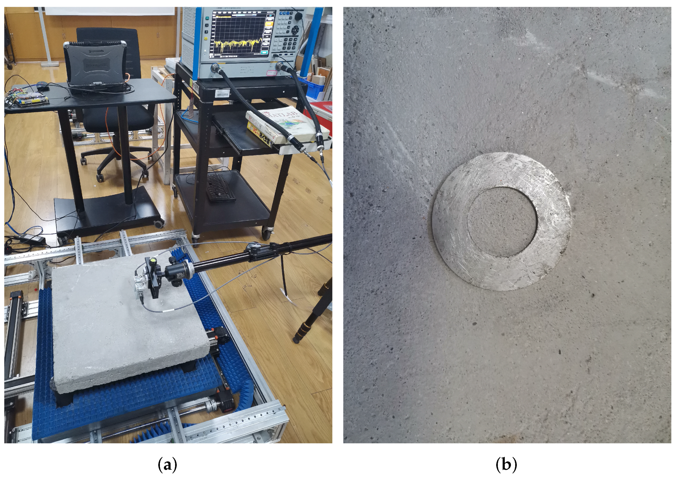
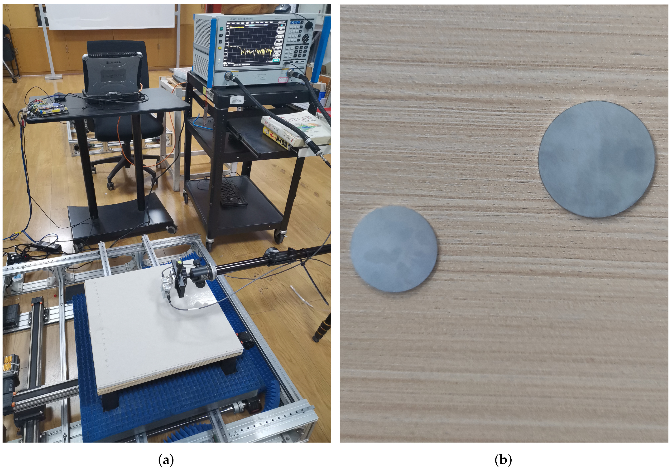
3.1. Experimental Setup

In addition to Scene II, two other real radar data were collected at our laboratory to validate the performance of the proposed method on detecting multi-targets and complicated-shaped targets. One test set was acquired from a scene with two targets behind the simulated wall (Scene III). Targets of interest consisted of two metal circles with the diameters of 3 cm and 4 cm, respectively. A 2-cm-thick pine wood and a 1-cm-thick gypsum slab partition were incorporated into the wall. Another data set used a model pistol as the target, which was overlapped with several paper documents and buried in a handbag (Scene IV). The antennas were kept 3 cm above the media surface and moved 40 steps at an interval of 0.6 cm along the 2D horizontal directions. The generated stepped-signal has a bandwidth of 20 GHz centered at 20 GHz. Figure 8 and Figure 9 present the photographs of the measurement setup of Scene III and Scene IV, respectively.

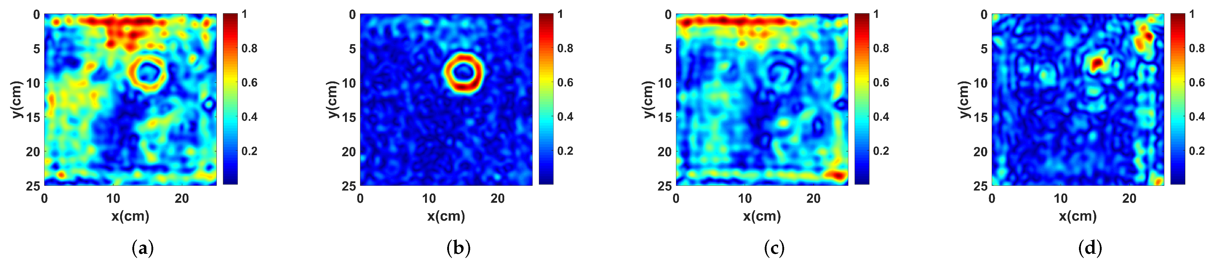
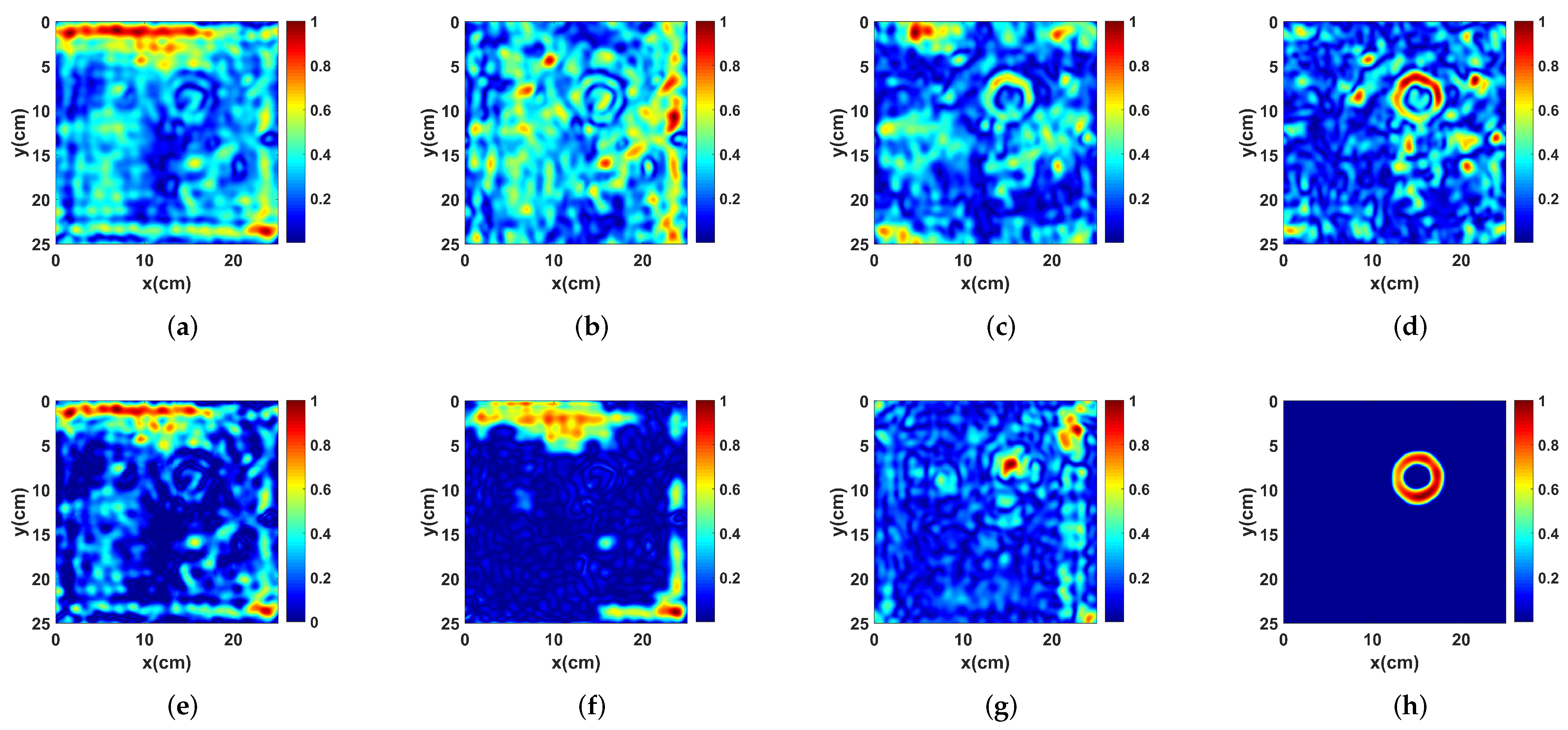
3.2. Performance Analysis and Comparison

For comparison purposes, six baseline methods, including PCA [16], the standard SVD [13], the adaptive SVD [29], RPCA [21], MCA [19], and the standard autoencoder [38], were implemented and evaluated on the same test scene. Figure 10 shows the obtained images at 10 GHz before and after clutter mitigation of Scene II. The dataset comprising 5000 holographic images mentioned above was used to training the autoencoder.
As shown in Figure 10a, we can hardly see the ring target in the imaging result of Scene II because the target response is much weaker than the surface reflections. The output images acquired from subspace projection methods are displayed in Figure 10b–d. Though the clutter subspaces are estimated to be reduced, the images of target in Figure 10b–d are still destroyed by the clutter to varying degrees. Figure 10e depicts the result of the RPCA method; since the clutter in the holographic image has irregular shapes, it is difficult to achieve a low-rank matrix to remove the clutter. The result of the MCA method is shown in Figure 10f, where most of the clutter is suppressed but target is also removed, demonstrating that constructing adaptive subdictionaries to separate the clutter and target component in HSR images is still a open issue. The standard autoencoder fails to extract the target feature because the response is too weak to be detected, as is shown in Figure 10g. After applying the proposed method, the result is presented in Figure 10h, where the clutter is completely removed without compromising the target image. A quantitative analysis of different clutter mitigation methods in terms of SCR is listed in Table 1. Among these seven methods, the proposed method produces the best SCR of 32.5 dB, followed by the adaptive SVD with a SCR of 7.2 dB. Though the standard autoencoder achieves the third highest SCR of 4.4 dB, it distorts the target shape, which is unacceptable for subsurface objects detection.
The holographic images of Scene III at 11 GHz are presented in Figure 11. Without any preprocessing, Figure 11a depicts an image where the target response is obscured by strong clutter. With the availability of subspace projection methods, part of the strong clutter is removed, and the target signatures in the hologram obtained from the adaptive SVD are stronger than those from PCA and the standard SVD, as is shown in Figure 11b–d. This is because PCA and the standard SVD assume that the wall clutter only resides in the first subspace while the reflections backscattered from a heterogeneous wall have been proved to span a multidimensional subspace which is difficult to be accurately estimated [14]. Figure 11e,f shows the results obtained using RPCA and MCA. Though the relatively weak clutter is reduced effectively, chunk clutter still remains in the processed images because both methods capture the sparse components in the radar data to represent the targets. However, the clutter can scatter in various sizes and shapes if the holographic images are not preprocessed. The results in Figure 11g,h show that the autoencoder-based methods not only successfully mitigate the strong clutter but also preserve the target responses. Compared to the standard autoencoder, the proposed method performs slightly better in terms of producing a clearer target image and revealling the reflections of the circle metals. The SCRs of these methods listed in Table 1 also demonstrate the effectiveness of our proposed method. Specifically, the SCR improvement over the standard autoencoder, RPCA, the adaptive SVD, MCA, PCA, and the standard SVD is 11.1, 21.1, 23.3, 23.5, 25.1, and 25.5 dB, respectively.
Figure 12 depicts the holographic images of Scene IV at 17 GHz before and after clutter mitigation. Without clutter mitigation, the target shape in the image shown in Figure 12a is barely identifiable compared with that in Figure 12b–d, which present the results after applying PCA, the standard SVD, and the adaptive SVD methods for clutter removal, respectively. Among these subspace projection methods, the adaptive SVD achieves the best performance and successfully reconstructs the pistol-like target image due to the subspace identification based on the cross-correlation characteristics of radar signal. However, the scattered clutter is increased when the subspace is removed. Figure 12e,f illustrates that RPCA and MCA can effectively suppress the scattered clutter but fail to recover the target response which is obscured by strong interference. It can be seen in Figure 12g that the standard autoencoder reconstructs two chunk targets instead of the pistol shape, while the proposed method yields a relatively accurate target image because the training data are modified to improve the generalization ability of the autoencoder, as shown in Figure 12h. Since the targets are not well recognized in the above images, Figure 12i presents the result of background subtraction as an extra reference. Though our proposed method still obtains the highest SCR on Scene IV compared with the other clutter mitigation methods, the SCR improvement is much lower than those on Scene II and Scene III, which demonstrates the proposed method achieves better performance when the target shape is regular or standardized.

3.3. Effect of Training Data

In general, the generalization ability of trained neural networks is related to the amount of training data. Therefore, the amount of training data can also affect the performance of proposed learning-based clutter mitigation method. To investigate the influence of training data, five datasets are constructed with different amounts of training radar signals. Set I contains 1000 radar images acquired from 10 different test scenes (In each scene, we obtained 100 training images by setting different kinds of targets or targets at different locations with a certain type of of medium such as concrete, planks, bricks, etc.). Various targets and materials are used in the test scenes. Similarly, Set II, III, IV, and V comprise 2000, 5000, 8000, and 10,000 radar signals obtained from the same 10 scenes (In each scene we obtained 200, 500, 800, and 1000 training images by setting different kinds of targets or targets at different locations with a certain type of of medium such as concrete, planks, bricks, etc.), respectively. After training the learning-based model with these datasets, we applied the proposed method on Scene I to IV and evaluate the performance in terms of SCR, which is presented in Table 2.
From Table 2, it can be clearly seen that SCR of the proposed method can be improved by increasing the amount of training data. Trained on these datasets, on average, the SCR is improved by 8.0 dB when the amount of training data is increased from 1000 to 2000, whereas the improvement falls to 0.55 dB when the amount of training data is increased from 8000 to 10,000. This slight improvement in SCR indicates that the proposed model does not require a large quantity of training sets to achieve good performance.

3.4. Discussion

The qualitative and quantitative results of Section 3 clearly demonstrate that the proposed method can effectively mitigate the clutter and improve the SCR. This superiority is attributed to the learning-based model and the availability of training dataset comprising of cluttered radar images captured in diverse scenes and the corresponding clean images obtained by background subtraction. In addition, with the assistance of the adaptive SVD, strongest clutter in HSR images can be preprocessed, thereby reducing redundant information and improving the extraction of salient information. Furthermore, the sparse representation is also combined to further optimize the model and the alternating direction multiplier method (ADMM) is used to solve the optimization problem for precision and efficiency. Though reconstructing the target image of irregular shape is still a challenge because the analytic model is not considered in the proposed method, as is shown in Figure 12, experiments carried out on several datasets demonstrate that the proposed method achieves superior performance in mitigating the strong clutter in HSR images with the target preserved compared with the existing clutter mitigation methods in terms of SCR.

4. Conclusions

In this paper, a learning-based clutter mitigation method is proposed for holographic subsurface imaging. First, an autoencoder-based clutter mitigation scheme is presented. Then, taking advantage of the adaptive SVD, the performance of autoencoder in extracting the target response is improved when the useful signal overlaps with strong clutter. The sparse representation is also combined to further enhance the sparse target profile and the ADMM method is used to solve the optimization problem for precision and efficiency. Both visual and quantitative results on real data have demonstrated that, compared with the existing clutter mitigation methods, the proposed method achieves superior performance on mitigating the strong clutter in HSR images with the target preserved. Future work will focus on improving the method with a more suitable neural network to reconstruct the irregular target signature.

Author Contributions

Conceptualization, C.C. and Y.L.; methodology, C.C.; software, C.C. and T.L.; validation, C.C., B.Y. and T.L.; formal analysis, C.C.; investigation, C.C.; resources, C.C. and Y.L.; data curation, C.C.; writing—original draft preparation, C.C.; writing—review and editing, C.C., B.Y. and T.L.; visualization, C.C.; supervision, Y.S.; project administration, T.L.; funding acquisition, T.L. All authors have read and agreed to the published version of the manuscript.

Funding

This research was funded by National Natural Science Foundation of China under Contract No.61901501.

Data Availability Statement

Not applicatable.

Conflicts of Interest

The authors declare no conflict of interest.

References

  1. Catapano, I.; Ludeno, G.; Soldovieri, F.; Tosti, F.; Padeletti, G. Structural assessment via ground penetrating radar at the Consoli Palace of Gubbio (Italy). Remote Sens. 2017, 10, 45. [Google Scholar] [CrossRef] [Green Version]
  2. Ho, K.C.; Gader, P.D. A linear prediction land mine detection algorithm for hand held ground penetrating radar. IEEE Trans. Geosci. Remote Sens. 2002, 40, 1374–1384. [Google Scholar] [CrossRef]
  3. Feng, X.; Sato, M.; Liu, C.; Takahashi, K.; Zhang, Y. Topographic correction of elevated GPR. IEEE J. Sel. Top. Appl. Earth Obs. Remote Sens. 2014, 7, 799–804. [Google Scholar] [CrossRef]
  4. Núñez-Nieto, X.; Solla, M.; Gómez-Pérez, P.; Lorenzo, H. GPR signal characterization for automated landmine and UXO detection based on machine learning techniques. Remote Sens. 2014, 6, 9729–9748. [Google Scholar] [CrossRef] [Green Version]
  5. Zhu, S.; Huang, C.; Su, Y.; Sato, M. 3D ground penetrating radar to detect tree roots and estimate root biomass in the field. Remote Sens. 2014, 6, 5754–5773. [Google Scholar] [CrossRef] [Green Version]
  6. Jadoon, K.; Weihermüller, L.; McCabe, M.; Moghadas, D.; Vereecken, H.; Lambot, S. Temporal monitoring of the soil freeze-thaw cycles over a snow-covered surface by using air-launched ground penetrating radar. Remote Sens. 2015, 7, 12041–12056. [Google Scholar] [CrossRef] [Green Version]
  7. Ivashov, S.; Razevig, V.; Vasilyev, I.; Zhuravlev, A.; Bechtel, T.; Capineri, L. Holographic subsurface radar of RASCAN type: Development and applications. IEEE J. Sel. Top. Appl. Earth Obs. 2011, 4, 763–778. [Google Scholar] [CrossRef]
  8. Huang, C.; Liu, T. The impact of an uneven medium surface in holographic penetrating imaging and a method to eliminate the interference. In Proceedings of the IEEE International Conference of IEEE Region 10 (TENCON 2013), Xi’an, China, 22–25 October 2013; pp. 1–4. [Google Scholar]
  9. Kovalenko, V.; Yarovoy, A.G.; Ligthart, L.P. A novel clutter suppression algorithm for landmine detection with GPR. IEEE Trans. Geosci. Remote Sens. 2007, 45, 3740–3751. [Google Scholar] [CrossRef]
  10. Solimene, R.; Cuccaro, A.; DellAversano, A.; Catapano, I.; Soldovieri, F. Ground clutter removal in GPR surveys. IEEE J. Sel. Top. Appl. Earth Obs. Remote Sens. 2014, 7, 792–798. [Google Scholar] [CrossRef]
  11. Brunzell, H. Detection of shallowly buried objects using impulse radar. IEEE Trans. Geosci. Remote Sens. 1999, 37, 875–886. [Google Scholar] [CrossRef] [Green Version]
  12. Daniels, D.J. Ground Penetrating Radar, 2nd ed.; IEEE: London, UK, 2004. [Google Scholar]
  13. Abujarad, F.; Nadimy, G.; Omar, A. Clutter reduction and detection of landmine objects in ground penetrating radar data using singular value decomposition. In Proceedings of the 3rd International Workshop on Advanced Ground Penetrating Radar, Delft, The Netherlands, 2–3 May 2005; pp. 37–42. [Google Scholar]
  14. Riaz, M.; Ghafoor, A. Through-wall image enhancement based on singular value decomposition. Int. J. Antennas Propag. 2012, 4, 1–20. [Google Scholar] [CrossRef]
  15. Tivive, F.; Bouzerdoum, A.; Amin, M. A subspace projection approach for wall clutter mitigation in through-the-wall radar imaging. IEEE Trans. Geosci. Remote Sens. 2015, 53, 2108–2122. [Google Scholar] [CrossRef] [Green Version]
  16. Lu, Q.; Pu, J.; Wang, X.; Liu, Z. A clutter suppression algorithm for GPR data based on PCA combining with gradient magnitude. Appl. Mech. Mater. 2014, 644–650, 1662–1667. [Google Scholar] [CrossRef]
  17. Zhao, A.; Jiang, Y.; Wang, W. Exploring independent component analysis for GPR signal processing. In Proceedings of the Progress in Electromagnetics Research Symposium, Hangzhou, China, 22–26 August 2005; pp. 750–753. [Google Scholar]
  18. Chen, W.; Wang, W.; Gao, J.; Xu, J. GPR clutter noise separation by statistical independency promotion. In Proceedings of the 14th International Conference on Ground Penetrating Radar, Shanghai, China, 4–8 June 2012; pp. 367–370. [Google Scholar]
  19. Zhou, Y.; Chen, W. MCA-based clutter reduction from migrated GPR data of shallowly buried point target. IEEE Trans. Geosci. Remote Sens. 2019, 57, 432–448. [Google Scholar] [CrossRef]
  20. Candès, E.J.; Li, X.; Ma, Y.; Wright, J. Robust Principal Component Analysis? J. ACM 2011, 58, 11. [Google Scholar] [CrossRef]
  21. Song, X.; Xiang, D.; Zhou, K.; Su, Y. Improving RPCA-based clutter suppression in GPR detection of antipersonnel mines. IEEE Geosci. Remote Sens. 2017, 17, 1338–1442. [Google Scholar] [CrossRef]
  22. Zhang, Z.; Ely, G.; Aeron, S.; Hao, N.; Kilmer, M. Novel methods for multilinear data completion and de-noising based on Tensor-SVD. In Proceedings of the 2014 IEEE Conference on Computer Vision and Pattern Recognition, Columbus, OH, USA, 23–28 June 2014; pp. 3842–3849. [Google Scholar]
  23. Lu, C.; Feng, J.; Chen, Y.; Liu, W.; Lin, Z.; Yan, S. Tensor robust principal component analysis: Exact recovery of corrupted low-Rank tensors via convex optimization. In Proceedings of the 2016 IEEE Conference on Computer Vision and Pattern Recognition, Las Vegas, NV, USA, 27–30 June 2016; pp. 5249–5257. [Google Scholar]
  24. Wei, D.; Wang, A.; Feng, X.; Wang, B. Tensor completion based on triple tubal nuclear Norm. Algorithms. 2018, 11, 94. [Google Scholar] [CrossRef] [Green Version]
  25. Zhang, L.; Peng, Z. Infrared small target detection based on partial sum of the tensor nuclear norm. Remote Sens. 2019, 11, 382. [Google Scholar] [CrossRef] [Green Version]
  26. Vishwakarma, S.; Ummalaneni, V.; Iqbal, M.; Majumdar, A.; Ram, S. Mitigation of through-wall interference in radar images using denoising autoencoders. In Proceedings of the 2018 IEEE Radar Conference (RadarConf18), Oklahoma City, OK, USA, 23–27 April 2018; pp. 1543–1548. [Google Scholar]
  27. Ni, Z.; Ye, S.; Shi, C.; Li, C.; Fang, G. Clutter suppression in GPR B-Scan images using robust autoencoder. IEEE Geosci. Remote Sens. 2020, 19, 3500705. [Google Scholar] [CrossRef]
  28. Tivive, F.; Bouzerdoum, A. Clutter removal in through-the-wall radar imaging using sparse autoencoder with low-rank projection. IEEE Trans. Geosci. Remote Sens. 2021, 59, 1118–1129. [Google Scholar] [CrossRef]
  29. Chen, C.; He, Z.; Song, X.; Liu, T.; Su, Y. A subspace projection approach for clutter mitigation in holographic subsurface imaging. IEEE Geosci. Remote Sens. 2022, 19, 1–5. [Google Scholar] [CrossRef]
  30. Boyd, S.; Parikh, N.; Chu, E.; Peleato, B.; Eckstein, J. Distributed Optimization and Statistical Learning via the Alternating Direction Method of Multipliers. Found. Trends Mach. Learn. 2011, 3, 1–122. [Google Scholar] [CrossRef]
  31. Tivive, F.; Bouzerdoum, A.; Abeynayake, C. GPR target detection by joint sparse and low-rank matrix decomposition. IEEE Trans. Geosci. Remote Sens. 2019, 57, 2583–2595. [Google Scholar] [CrossRef] [Green Version]
  32. Snoek, J. Scalable Bayesian optimization using deep neural networks. In Proceedings of the 32nd International Conference on Machine Learning, Lille, France, 7–9 July 2015; pp. 2171–2180. [Google Scholar]
  33. Czarnecki, W.; Podlewska, S.; Bojarski, A. Robust optimization of SVM hyperparameters in the classification of bioactive compounds. J. Cheminform. 2015, 57, 1–15. [Google Scholar] [CrossRef] [PubMed] [Green Version]
  34. Yao, C.; Cai, D.; Bu, J.; Chen, G. Pre-training the deep generative models with adaptive hyperparameter optimization. Neurocomputing 2017, 5247, 144–155. [Google Scholar] [CrossRef]
  35. Ivashov, S.I.; Capineri, L.; Bechtel, T.D.; Razevig, V.V.; Inagaki, M.; Gueorguiev, N.L.; Kizilay, A. Design and Applications of Multi-Frequency Holographic Subsurface Radar: Review and Case Histories. Remote Sens. 2021, 13, 3487. [Google Scholar] [CrossRef]
  36. Song, X.; Su, Y.; Zhu, C. Improving holographic radar imaging resolution via deconvolution. In Proceedings of the 15th International Conference on Ground Penetrating Radar, Brussels, Belgium, 30 June–4 July 2014; pp. 633–636. [Google Scholar]
  37. Song, X.; Su, Y.; Huang, C. Landmine detection with holographic radar. In Proceedings of the 16th International Conference on Ground Penetrating Radar (GPR), Hong Kong, China, 13–16 June 2016; pp. 1–4. [Google Scholar]
  38. Gondara, L. Medical image denoising using convolutional denoising autoencoders. In Proceedings of the 2016 IEEE 16th International Conference on Data Mining Workshops (ICDMW), Barcelona, Spain, 12–15 December 2016; pp. 241–246. [Google Scholar]
  39. Zhou, H.; Feng, X.; Dong, Z.; Liu, C.; Liang, W. Application of Denoising CNN for Noise Suppression andWeak Signal Extraction of Lunar Penetrating Radar Data. Remote Sens. 2021, 13, 779. [Google Scholar] [CrossRef]
  40. Meng, Z.; Zhan, X.; Li, J. An enhancement denoising autoencoder for rolling bearing fault diagnosis. Measurement 2018, 130, 448–454. [Google Scholar] [CrossRef] [Green Version]
  41. Ashfahani, A.; Pratama, M.; Lughofer, E. DEVDAN: Deep evolving denoising autoencoder. Neurocomputing 2020, 390, 297–314. [Google Scholar] [CrossRef] [Green Version]
  42. Zhu, W.; Mousavi, S.M.; Beroza, G.C. Seismic signal denoising and decomposition using deep neural networks. IEEE Trans. Geosci. Remote Sens. 2019, 57, 9476–9488. [Google Scholar] [CrossRef] [Green Version]
  43. Maleki, A.; Anitori, L.; Yang, Z.; Baraniuk, R. Asymptotic analysis of complex LASSO via complex approximate message passing (CAMP). IEEE Trans. Inf. Theory 2013, 59, 4290–4308. [Google Scholar] [CrossRef] [Green Version]
  44. Snoek, J.; Larochelle, H.; Adams, R. Practical Bayesian optimization of machine learning algorithms. In Proceedings of the 25th International Conference on Neural Information Processing Systems, Lake Tahoe, NV, USA, 3–6 December 2012; pp. 2951–2959. [Google Scholar]
  45. Kemp, C.; Matern, B. Spatial Variation. J. R. Stat. Soc. A. Stat. D 1988, 37, 84. [Google Scholar] [CrossRef]
  46. Mockus, J.; Tiesis, V.; Zilinskas, A. The application of Bayesian methods for seeking the extremum. Towards Glob. Optim. 1978, 2, 117–129. [Google Scholar]
Figure 1. Geometry of holographic subsurface radar system.
Remotesensing 14 00682 g001
Figure 2. Architecture of an autoencoder. The input layer receives a cluttered image X and reconstructs the output target image X ^ with the latent-space representation.
Remotesensing 14 00682 g002
Figure 3. Photograph of measurement setup of Scene I. (a) View of the test scene. (b) Hidden target.
Remotesensing 14 00682 g003
Figure 4. HSR images obtained from different clutter before and after using the standard autoencoder. (a) Imaging result of Scene I. (b) Autoencoder result of Scene I. (c) Imaging result of Scene II. (d) Autoencoder result of Scene II.
Remotesensing 14 00682 g004
Figure 5. HSR images obtained from the standard autoencoder with double the amount of training data. (a) Autoencoder result of Scene I. (b) Autoencoder result of Scene II.
Remotesensing 14 00682 g005
Figure 6. HSR images obtained from the adaptive SVD and denoizing autoencoder on Scene II. (a) Result of the adaptive SVD. (b) Result of the denoizing autoencoder.
Remotesensing 14 00682 g006
Figure 7. Structure of the proposed learning-based clutter mitigation with subspace projection and sparse representation. (Words in the blue box indicate the above datasets or models, whereas words in the red box indicate the procedures).
Remotesensing 14 00682 g007
Figure 8. Photograph of measurement setup of Scene III. (a) View of the test scene. (b) Hidden targets.
Remotesensing 14 00682 g008
Figure 9. Photograph of measurement setup of Scene IV. (a) View of the test scene. (b) Hidden target.
Remotesensing 14 00682 g009
Figure 10. HSR images of Scene II before and after using different clutter mitigation methods. (a) No clutter mitigation. (b) Result of PCA. (c) Result of the standard SVD. (d) Result of the adaptive SVD. (e) Result of RPCA. (f) Result of MCA. (g) Result of the standard autoencoder. (h) Result of the proposed method.
Remotesensing 14 00682 g010
Figure 11. HSR images of Scene III before and after using different clutter mitigation methods. (a) No clutter mitigation. (b) Result of PCA. (c) Result of the standard SVD. (d) Result of the adaptive SVD. (e) Result of RPCA. (f) Result of MCA. (g) Result of the standard autoencoder. (h) Result of the proposed method.
Remotesensing 14 00682 g011
Figure 12. HSR images of Scene IV before and after using different clutter mitigation methods. (a) No clutter mitigation. (b) Result of PCA. (c) Result of the standard SVD. (d) Result of the adaptive SVD. (e) Result of RPCA. (f) Result of MCA. (g) Result of the standard autoencoder. (h) Result of the proposed method. (i) Result of background subtraction.
Remotesensing 14 00682 g012
Table 1. SCR of Different Clutter Mitigation Methods.
Scene IIScene IIIScene IV
None−3.3 dB2.2 dB4.4 dB
PCA−1.1 dB3.2 dB4.2 dB
The standard SVD2.9 dB2.8 dB4.8 dB
The adaptive SVD7.2 dB5.0 dB5.7 dB
RPCA−5.8 dB7.2 dB6.9 dB
MCA−3.2 dB4.8 dB6.7 dB
The standard autoencoder4.4 dB17.2 dB8.1 dB
The proposed method32.5 dB28.3 dB10.0 dB
Table 2. SCR of the proposed method with different amounts of training data.
Training DatasetNumber of DataSCR
Scene IScene IIScene IIIScene IV
Set I100015.1 dB13.4 dB18.9 dB6.9 dB
Set II200032.8 dB18.9 dB25.1 dB9.5 dB
Set III500033.4 dB32.5 dB28.3 dB10.0 dB
Set IV800034.1 dB32.8 dB32.1 dB10.7 dB
Set V10,00034.2 dB32.9 dB33.4 dB11.4 dB
Publisher’s Note: MDPI stays neutral with regard to jurisdictional claims in published maps and institutional affiliations.

