
3D Lightning Location Method Based on Range Difference Space Projection

1
School of Computer Science, Chengdu Normal University, Chengdu 611130, China
2
Key Laboratory of Interior Layout Optimization and Security, Institutions of Higher Education of Sichuan Province, Chengdu Normal University, Chengdu 611130, China
*
Author to whom correspondence should be addressed.
Remote Sens. 2022, 14(4), 1003; https://doi.org/10.3390/rs14041003
Submission received: 11 January 2022
/
Revised: 13 February 2022
/
Accepted: 16 February 2022
/
Published: 18 February 2022
(This article belongs to the Special Issue Remote Sensing of Lightning and Its Applications in Atmospheric Electricity Studies)
Abstract
:Most lightning location networks obtain the position results by optimizing the goodness of fit to determine that all combinatorial time differences of arrivals (TDOAs) are due to a common discharge. This paper proposes a three-dimensional (3D) lightning location method based on range difference (RD) space projection. The proposed method projects all the measurements into the RD space, which has the space-invariant feature of the equivalence cell and can be partitioned soundly. Aiming at the problem of computational cost of the procedure of the projection, the hierarchical strategy is proposed to improve computational efficiency. The performance of the RD space projection based on the hierarchical strategy is analyzed via Monte-Carlo simulations. The results show that the proposed method can locate lightning sources in real time with high accuracy. The results also show that the location accuracy is limited by the level of the inherent time uncertainty, the layout, and the size of the receiver network. Under the fixed layout and size of the receiver network, and the fixed measurement noise uncertainty, the positioning precision cannot be improved more even if the grid step is small enough or the number of receivers is large enough.

1. Introduction
Lightning is a kind of strong discharge phenomenon occurring in convective weather, which is one of the most common disastrous weather phenomena in nature. With the wide application of microelectronic equipment and electrical equipment, the direct and indirect disasters caused by lightning are becoming more and more serious. Therefore, the detection and early warning of lightning have become urgent tasks to be solved.
The three-dimensional (3D) location technology of lightning provides key information for the research of the development mechanism of the lightning and early warning of the lightning because it not only can monitor the cloud-to-ground lightning (CG) well, but it can also observe the development process by using early lightning electromagnetic radiation during intra-cloud lightning (IC) [1,2,3,4]. Therefore, various studies have recently been carried on the fine location technology of the total lightning. The representative location systems are Lightning Mapping Array (LMA) system and Los Alamos Sferic Array (LASA) system. The LMA system adopted the time difference of arrival (TDOA) technique that is based on GPS clock synchronization and can detail the lightning channel structure [5,6,7,8]. The LASA system is a fast electric field location network in the VLF/LF band and is capable of high-precision, three-dimensional locations of total lightning discharge using the TOA method [9,10,11]. Later, a series of similar detection systems have been developed around the world, including the Huntsville Alabama Marx Meter Array, a Broadband Observation network, an LF near-field interferometric-TOA 3D Lightning Mapping Array, etc. [12,13,14,15,16,17,18,19]. Based on the above work, Fan et al. introduced a signal processing method (empirical mode decomposition (EMD) technology) to filter the original waveform to improve the accuracy of the peak time extraction, which further improves the location accuracy [18]. Furthermore, the time reversal (TR) technology can also be used in the 3D location of lightning discharges [20,21,22]. For example, Chen et al. used the TR method to find the optimal solution in the space limited by the linear initial solution of the TOA method [21]. Li et al. combined the TDOA technique and electromagnetic TR technique to image lightning channels [22]. In addition, the deep-learning technology has been introduced in the location of total lightning [23]. The ABA (A, B double time base) data acquisition system based on first input first output memory is adopted in a low frequency 3D lightning mapping network [24].
The lightning location based on the TOA technique can be roughly divided into two categories. The one works by solving a group of non-linear equations by some iteration [23,25,26] or analytical algorithm in principle [27,28], and the other adopts the numerical grid traverse algorithm (GTA), which builds a grid database first and then finds the grid point that matches the time differences [15,29]. Different from the iteration algorithm, the GTA does not need an initial value and is inherently accurate but has computing burdensome. Qin et al. proposed a GPU-based GTA algorithm, which has a fast location speed, although the matching ability is not improved [30].
Recently, multi-target positioning for a passive sensor network via bistatic range (BR) space projection is proposed [31,32]. This method uses the projection strategy to solve multi-target positioning problems in the viewpoint of the imaging technique. Projection strategy is the traversal method and similar to the GTA, which partitions the surveillance region into a group of grids and substitutes the grid point into equations. However, the difference between the projection strategy (PS) and GTA is that GTA obtains the positioning results by optimizing the objective function, and PS accumulates the vote for each grid and picks up the grid that has the maximum vote value as the positioning results. In addition, the BR space projection method is proposed to eliminate the space-variant feature in the geographic space in the face of a vast surveillance region.
Based on the work of [31,32], in this study, we propose a 3D lightning location method based on the range difference (RD) space projection. We present a detailed derivation procedure of the space-variant feature in the geographic space and project the TDOAs into the RD space, which is space-invariant. Considering the computational cost, a hierarchical search strategy from coarse to fine is proposed. This method has fine location ability based on the analysis of the Monte Carlo simulation.
2. Model of TDOA Lightning Detection Sensor Network
The lightning location receiver network, based on TDOA, consists of (3) spatially separated receiver stations, which is illustrated in Figure 1. The sampled time series from all the receivers are synchronized using a GPS clock.
Since a TDOA-based positioning system does not measure absolute time, but instead measures the time difference that a signal arrives at the TDOA receivers with respect to the reference TDOA receiver, the TDOAs are expressed as
where is the absolute time of arrival to the reference receiver, is the absolute time that the lightning source arrives at the th receiver, and is the number of receivers, excluding the reference receiver (receiver 0). The TDOAs are converted to RDs by multiplying by , the speed of light in air:
where is the RDs of the lightning source to the th receiver and the reference receiver.
Assuming that the receivers’ positions are given, we have
where, denotes the positions of the th receiver, denotes the reference receiver that is located at the origin of the coordinates, denotes the position of the lightning source, denotes the range of the th receiver and the lightning source, denotes the range of the reference receiver and the lightning source, and means 2-norm.
Considering the reference receiver is located at the origin, one can create the RD equations by combining all the receivers’ information as:
Equation (4) is a group of hyperbolic equations that can be solved by some iteration [23,25,26] or analytical algorithm [27,28]. Unfortunately, we cannot determine that all the observed TDOAs are due to a common discharge because there might have been flipping and superposition in the different receivers. Flipping is caused by the change of relative positions of the receivers and the lightning sources. Superposition is caused by the coinciding of the different lightning flashes in some receivers. Flipping and superposition might cause some TDOAs that should be used more than once when creating the RD equation, which indicates that the relative position cannot be used as a rule to allocate TDOAs. Besides these, there might be some false TDOAs in the echoes because of the existence of noise.
Since a TDOA may participate in multiple combinations in the calculation at the same time, leading to multiple location results, the goodness of fit is compared in all combinations to select the best result [13,28]. However, flipping, superposition, and false echoes lead to the idea that there might be dozens of candidate TDOAs in practice, and the combination of the possible RD equations is considerable (assume that there are ten receivers and five candidates for every receiver, the number of the possible RD equations is 510). Thus, we must find some new ways to solve the lightning location problem.
3. Geographic Space Projection
3.1. Geographic Space Projection
Differing from the iteration algorithm to solve the non-linear equations, the traversing algorithm discretizes the network region into a series of grids, finds the grid point that matches the TDOAs, and then votes the corresponding grid. After traversing all of the grids and equations, the grids whose votes are equal to the number of equations is the solution of the equations.
In fact, the traversing strategy is popular in the microwave imaging processing field, such as the back projection algorithm [33]. Thus, the multi-target location problem can be solved by some classical imaging algorithm, such as the back projection algorithm [34,35], which is illustrated in Figure 2.
Based on the back projection algorithm, a geographic projection is proposed, and the steps are listed as follows:
- Step 1.
- Partition the solution region into a group of grids by the grid step and assign a representative for each of them.
- Step 2.
- Select one representative, calculate its’ TDOA according to Equation (4). Compare the calculated TDOA with the observed TDOA ; if the absolute difference is less than the designated threshold , , the representative gets a vote, if else do nothing.
- Step 3.
- Change the receiver one by one and repeat step 2 until all receivers are processed.
- Step 4.
- Change the representative one by one and repeat steps 2 and 3 until the whole solution domain is processed.
- Step 5.
- Select the representatives whose value of vote is greater than the designated threshold . The coordinates of those representatives are the estimated lightning sources’ position.
A discretized 2D region is illustrated in Figure 3.
3.2. Equivalence Cell
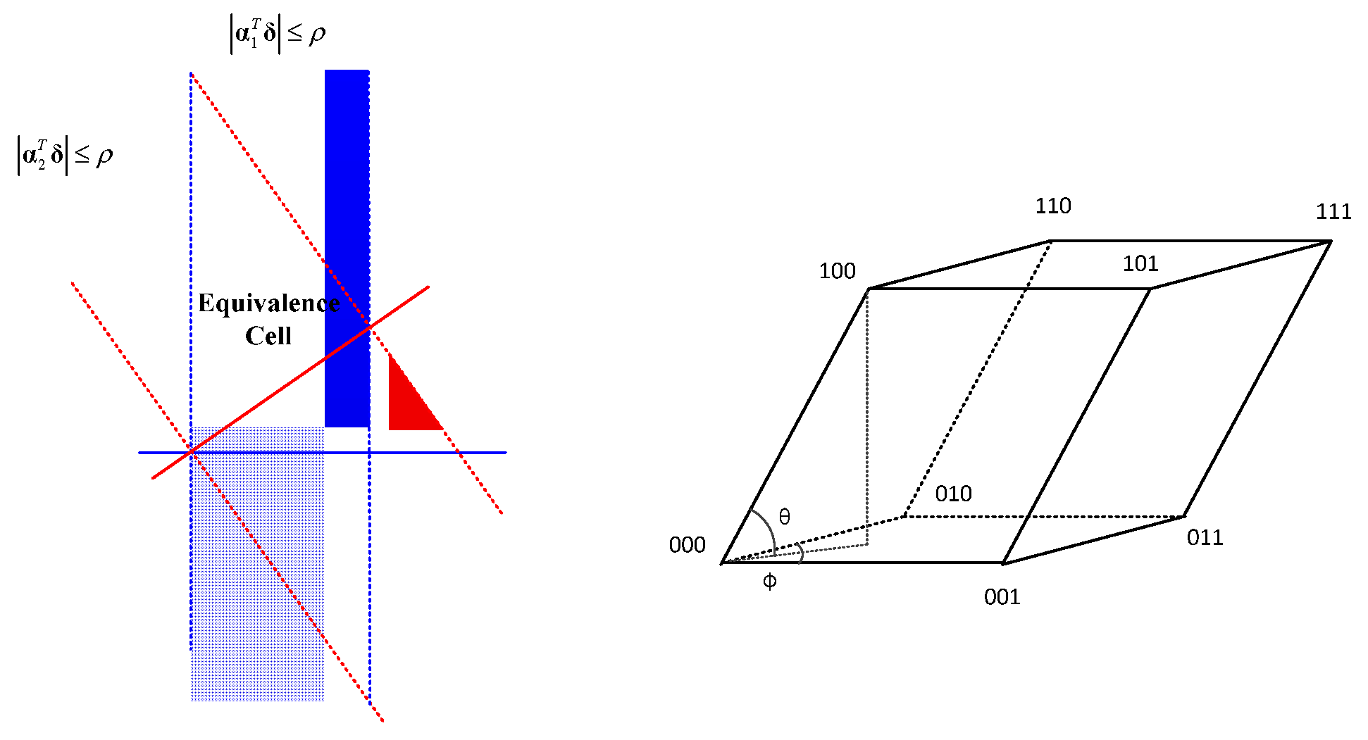
Because of the discretization of the surveillance region, the RD equation should be rewritten as a group of inequalities in practice:
where is the variable, and denotes the grid step. The collection of those satisfying the inequalities is named as ambiguity region in the field of imaging processing. Obviously, given a representative , all those positions in the same ambiguity region are indistinguishable and should be partitioned into the same grid, which is named as equivalence cell in this paper.
By introducing a group of intermediate variables , the equivalence cell can be considered as a mapping from a high-dimensional cube into the 3D space, i.e.,:
where, , which is a N-dimensional cube.
Given a representative , by the multivariate Taylor expansion theorem, can be approximated as:
Equations (8) to (10) indicate that the equivalence cell of the geographic space projection is approximately a polygon in 3D space.
To facilitate the analysis, we present the following property (seeing Appendix A for details) at first.
Property 1.
Given three receivers whose positions are, , and, and assume that there is a pair ofandsatisfying:, and, then (approximately), where denotes a point in the triangle with vertices , , and .
Property 1 indicates that the shape of the equivalence cell is dominant by the three receivers covering the largest area. In other words, one cannot improve the positioning precision via increasing the number of receivers in the triangle (compatible with the discussion on the position dilution of precision (PDOP) [36] of GPS system).
Under this property, we can continue our discussion on the equivalence cell by examining only four receivers.
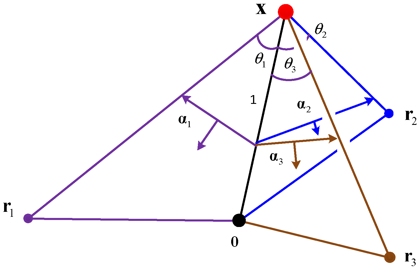
The geometry of is shown in Figure 4. Given a representative , receiver , and reference point 0, the associated with Equation (10) is the lower side of the isosceles triangle that is determined by the unit vectors of and . When the three sensors are not collinear, , , and are not co-planar. Thus, the equivalence cell is the linear transform of a cube, which is a parallel hexahedron and is shown in Figure 5. The eight vertices of the hexahedron can be calculated as:
where denotes the vertices of the cube.
Equation (11) indicates that the size of the equivalence cell is proportional to the grid step; the smaller the grid step is, the smaller the equivalence cell is. On the other hand, the equivalence cell is space-variant with respect to the representative (seeing Section 5 for details). This space-variant characteristic makes it difficult to partition the solution domain in the geographic space effectively. A fine partition means that there might be several representatives for some equivalence cells (for those regions far away from the receiver network); a coarse partition means that there might be no representative for some equivalence cells (for those regions near the receiver network). Thus, a novel projection algorithm is proposed in the next section.
4. RD Space Projection
According to the discussion in Section 3.2, it is difficult to partition the solution domain soundly, as the equivalence cell in the geographic space is irregular and space-variant. On the contrary, the equivalence cells of the intermediate variable (corresponding to the RD of different receivers) are all regular and space-invariant (N-dimensional cube). Therefore, we can project the data into the RD space, rather than the geographic space, which can be defined as:
where denotes the solution domain in the RD space, denotes the solution domain in the geographic space, and Equation (13) gives the mapping between the RD space and the geographic space. Obviously, given an or , there is only one or one (only one is reasonable) corresponding to it. Thus, we can traverse one by one to substitute traversing .
In the RD space, we can simply find a partition as:
where is the representative of .
For the (3) receivers network, the three whose triangle can cover as many other receivers as possible are selected, and their positions are used to create the mapping by Equation (13). According to Property 1, if an equivalence cell’s counterpart satisfies the equations in Equation (5) associated with the three sensors, it satisfies the other equations approximately too.
In addition, the geographic projection is computing costly and its overall performance, such as the speed and location precision, relies heavily on the grid step and the surveillance region. Therefore, we proposed the hierarchical search strategy to decrease the grid step and shrink the solution region gradually. At the first, we partition the solution domain by using the large grid step and obtain the coarse location. Then, we shrink the solution domain into some specific regions. We partition the new solution domain by using another smaller grid step and obtain the new location until the accuracy of the position result is satisfied the system requirement. The computational cost can be reduced geometrically by the hierarchical strategy iteratively.
According to the above discussion, the steps of the RD space projection based on hierarchical strategy are listed as follows:
- Step 1.
- Select three receivers whose triangle covers as many receivers as possible.
- Step 2.
- Calculate the representatives in the RD space according to Equation (16) and solve the non-linear Equation (13) to obtain representatives’ counterparts in the geographic space.
- Step 3.
- Calculate the RDs using the representatives’ counterparts via Equation (4) and perform the geographic space projection discussed in Section 3.1.
- Step 4.
- If the votes of the representatives are greater than the threshold, store the positions of them. Set a new solution domain with some specific size of a 3D cube and center at those positions. Change the grid step to a smaller one. Repeat step 1 to step 4 of the geographic space projection by using the new solution domain and the new grid step until the accuracy of the position result satisfies the system requirement. Then, the representatives’ positions whose votes are greater than the threshold are the estimated lightning sources’ positions.
5. Performance Analysis
5.1. Space-Invariant Feature of the RD Space
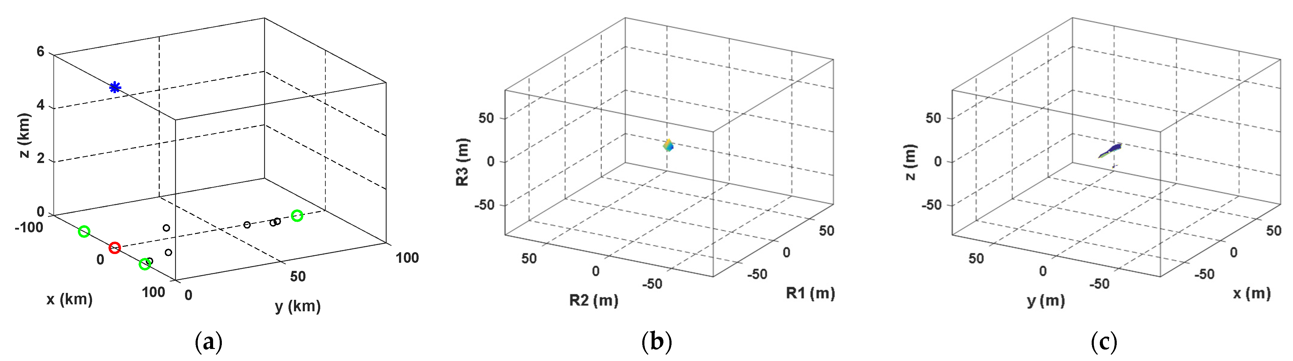
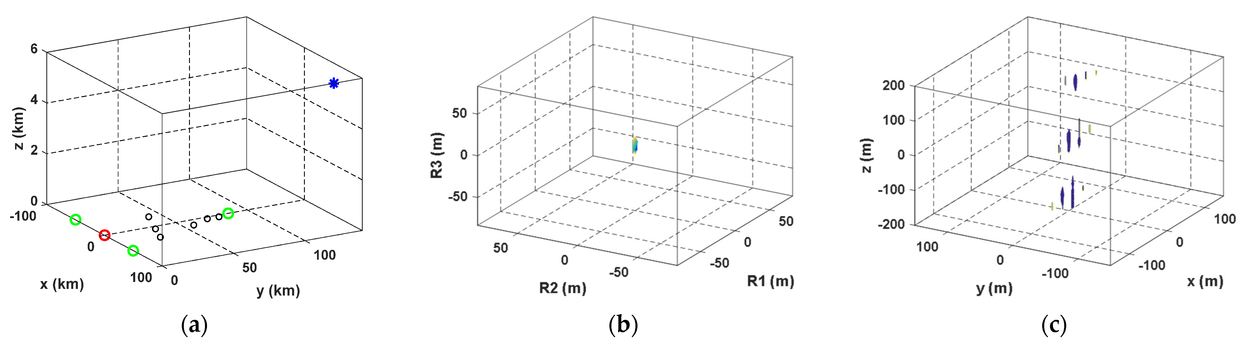
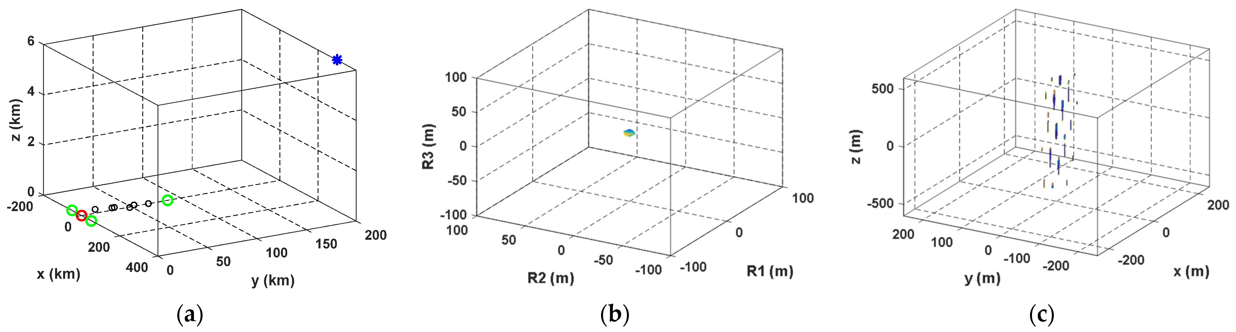
This subsection demonstrates the space-invariant feature of the RD space. Assume that there are 10 receivers. Figure 6, Figure 7, and Figure 8a plot geometries of the receiver network with the lightning flash, one of the receivers (the red circle) is placed at the origin, three of the receivers (the cyan circles) are located at [−50, 0, 0] km, [50, 0, 0] km, and [0, 87, 0] km. the others (the black circles) are distributed uniformly in the triangle determined by the three receivers, and the lightning flash (the blue star) is located at [0, 0, 6] km, [100, 120, 6] km, and [300, 200, 6] km, respectively. The equivalence cells (ambiguity region whose values are 0.7 times larger than the maximum value) in the RD space and the geographic space are shown in Figure 6, Figure 7, and Figure 8b,c respectively.
From Figure 6, Figure 7, and Figure 8, we find that the equivalence cells in both the RD space and the geographic space are points when the lightning source is located at [0, 0, 6] km. The equivalence cell in the geographic space diffuses significantly, but the one in the RD space is still a point when the source is located at [100, 120, 6] km. The equivalence cell in the geographic space diffuses in a mass region, but the one in the RD space is still a point when the source is located at [300, 200, 6] km.
Assume that the surveillance region ranges from [0, 0, 0] km to [300, 200, 6] km; if a coarse grid step is selected, some lightning sources located in those regions near to the receiver network might be lost. On the contrary, if a fine grid step is selected, a lot of projection operations are performed for an equivalence cell in those regions far from the network in the geographic space, which is useless for positioning. In the RD space, the equivalence cell can easily avoid the redundant operations and lightning source loss as it is space-invariant.
It is worth mentioning that, since one needs to solve the geographic positions from the coordinates in the RD space via Equation (13), the space-invariant feature of the RD space does not mean that its positioning precision is superior to that in the geographic space. The theoretical analysis on the positioning precision of the receiver network is similar to that of the GPS system, i.e., geometric dilution of precision (GDOP), position dilution of precision (PDOP), etc., which can be found in the literature [36]. Further discussion of the positioning precision is presented in Section 5.2 based on some numerical experiments.
5.2. Positioning Performance Analysis
This subsection discusses the influences of the additive timing noise, number of receivers, and lightning source positions on the positioning performance. The surveillance regions are from [−200, −200, 0] km to [200, 200, 10] km. Assume that there are 5, 10, 20, and 30 receivers, respectively; one of the receivers is placed at the origin, three of the receivers are located at [−50, −50, 0] km, [50, −50, 0] km, and [0, 50, 0] km, and the others are distributed uniformly in the triangle determined by the three receivers. The baseline of the network is 100 km. Use four-level hierarchical grids. The first-level grid is 41 × 41 × 10 with a grid step of 10 × 10 × 1km to cover the whole surveillance region. The second-level grid is 100 × 100 × 10 with a grid step of 1000 × 1000 × 1000 m, the third-level grid is 100 × 100 × 100 with a grid step of 100 × 100 × 100 m, and the fourth-level grid is 100 × 100 × 100 with a grid step of 10 × 10 × 10 m.
Firstly, we discuss that there must be just one lightning source in the surveillance region. For analysis, the different lightning source positions on the positioning performance partition the surveillance region into 41 × 41 × 10 grids by interval 10 × 10 × 1 km. Assume that the lightning flash occurred in each grid one by one, and each time the source’s height is fixed at 6 km in the z dimension.
The simulation steps are listed as follows:
- Step 1:
- Select one grid, record the geographic position, and substitute the position in the Equation (4) to calculate the TDOA.
- Step 2:
- Add some gauss noise with standard deviation 100 ns in TDOA calculated in Step 1 to simulate the real observed measurement (according to the GPS measurement error).
- Step 3:
- Use the RD space projection algorithm based on the hierarchical strategy discussed in Section 3.1 and Section 4.
- Step 4:
- Extract the cells whose voting values are greater than the threshold. Store those cells’ position as the estimated lightning source’s positions and the corresponding onset time.
- Step 5:
- Repeat step 2 to step 4 1000 times, calculate the root mean square error (RMSE) in x-y and z between the simulated lightning source position and the estimated source position. The x-y RMSE and the z RMSE were calculated according towhere , , and are the , and positions of the simulated lightning source; , , and are the x, y, and z positions of the estimated lightning source by the RD space projection at th and th simulation, respectively; is the number of times of Monte-Carlo simulation of step 2 to step 4; , is the cell’s number of the partitioned surveillance region; is the whole grids’ number.
- Step 6:
- Repeat step 1 to step 5 times, until all surveillance region grids are processed, store all , , and .
The maximum , , and with the number of receivers 5, 10, 20, and 30 outside and inside the receiver network are listed in Table 1 and Table 2, respectively.
From Table 1 and Table 2, we find that, as the grid step decreases, the is smaller and the location accuracy is higher. When the grid step is 10 × 10 × 10 m, the position results inside the network with 5, 10, 20, and 30 receivers are less than 38 m location accuracy as the Gaussian timing error is 100 ns, and the position results outside the network with 5, 10, 20, and 30 receivers are less than 38 m for the horizontal and less than 500 m for the vertical. To the authors’ knowledge, the results are sound because the location accuracy is ~100 m in the coverage region of the network and ~1000 m out of the coverage region of the network by the existing algorithms. In addition, due to the measurement error of the arrival time, we cannot improve the location accuracy by increasing the receivers or decreasing the grid step further. Besides, we find that when the grid steps are 10,000 × 10,000 × 1000 m, 1000 × 1000 × 1000 m, and 100 × 100 × 100 m iteratively, the location accuracy becomes significantly worse as the receiver decreased. The location errors outside the network are much larger than the location errors inside the network under the same receivers and the same grid step, and the vertical position accuracy is less than the horizontal position accuracy under 5 to 30 receivers and different grid steps no matter inside or outside the network, except for the results inside the network under the 10×10×10m grid step. Especially, the and outside the network are larger than the current grid interval. It means that when we center at the last estimated points, shrink the resolve domain into 100 × 100 × 100 with the last grid step, and start the next searching by using smaller interval, the true location of the flash may be out of the new resolve domain. Then, we must risk losing the lightning source at the next hierarchical searching.
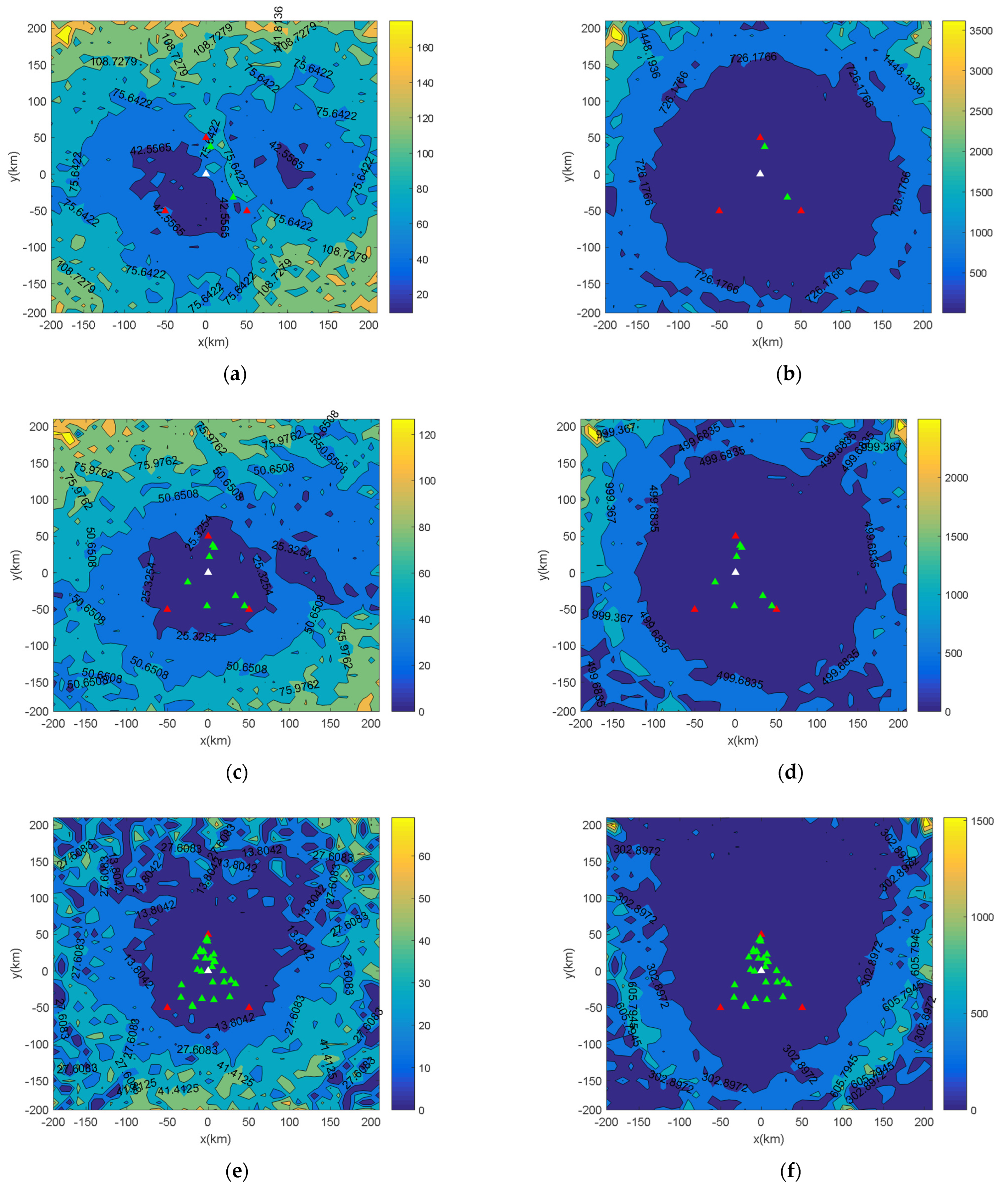
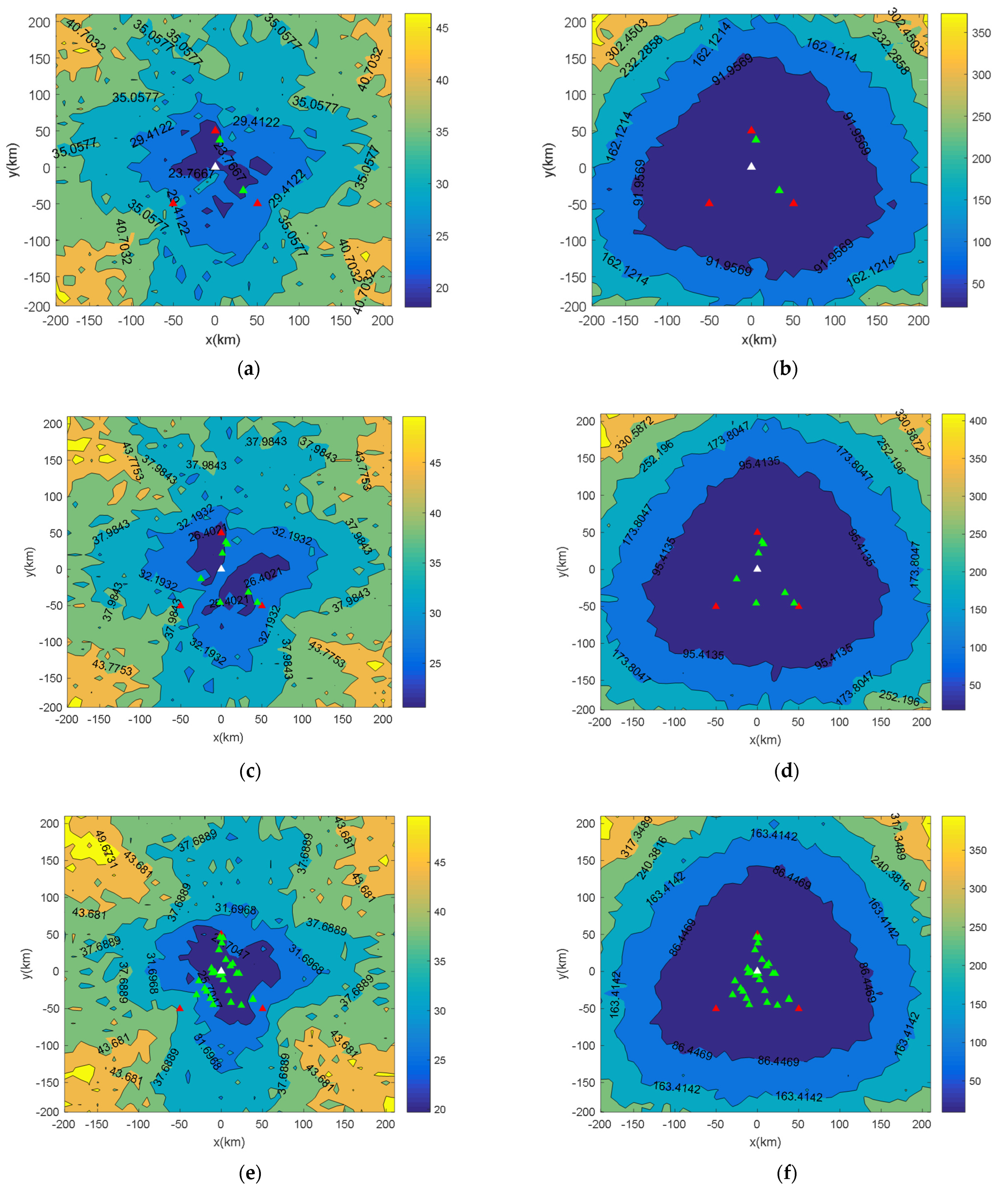
For discussing the location errors further, the location errors under 100 × 100 × 100 m grid searching step and 10 × 10 × 10 m grid searching step with 5, 10, and 30 receivers are plotted in Figure 9, and Figure 10, respectively. Figure 9, and Figure 10a,c,e are the horizontal location errors, and Figure 9, and Figure 10b,d,f are the vertical location errors. From Figure 9, and Figure 10, we find that, as the distance from the lighting source to the central station increases, the location accuracy gradually decreases. The and of the whole detection domain appear at the left and right corners. Figure 9, and Figure 10a,c,e show that the horizontal location error within a radius of 150 km is less than 50 m, and Figure 9, and Figure 10b,d,f show that the vertical location error within a radius of 150 km is less than 1000 m. This region is three times the baseline of the receiver network. The result can guide us to further subdivide the searching domain. For example, the searching domain in the radius of three times of the baseline can be set as 10 × 10 × 10 with the current grid step, and the searching domain out of the radius of three times of the baseline can be set as 100 × 100 × 100 with the current grid step, in order to not lose the source and balance the computational cost.
Computational cost is a big issue of the grid traverse algorithm. To balance the accuracy and computation, combining the results of Table 1 and Table 2, and Figure 9, and Figure 10, a 20 × 20 × 20 searching grid is accepted. Table 3 gives the processing time of one receiver for a one-time Monte-Carlo simulation. Because each receiver has the same computation procedure, it means N receivers can be processed parallelly. Therefore, under the parallel processing, the total processing time of the proposed algorithm is 0.8203 s. Moreover, for the first searching level, because the searching domain is fixed and determined by the user, we can calculate the results of the grid traverse and store them in advance. Then, the total processing time is reduced to 0.3536 s. It satisfies the requirement of the real-time lightning monitoring. Furthermore, we can divide the searching domain into two parts according to the results of Figure 9, and Figure 10 to reduce the computational cost further.
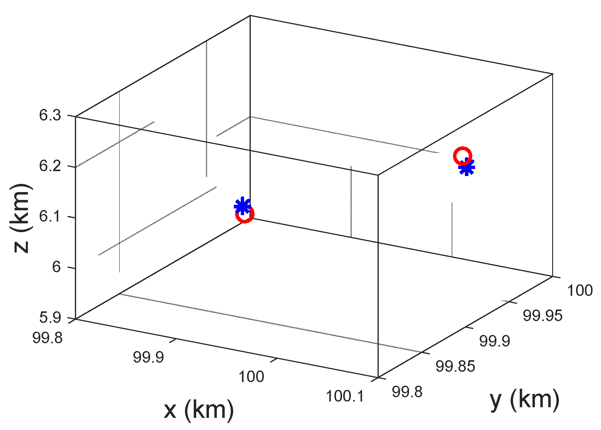
Finally, we discuss that there are two lightning sources in the surveillance region simultaneously. The 1000-time Monte-Carlo simulations are conducted with the standard deviation of timing noise 100 ns and the number of receivers 10. Two lightning flashes are distributed uniformly in a 3D cube with size 400 400 400 m3 and centered at [100, 100, 6] km. Figure 11 plots the positioning result of the RD space algorithm. From them, we find that the algorithm can position the two lightning sources correctly.
6. Conclusions
In this paper, a 3D lightning location method based on RD space projection, which combines with the hierarchical strategy, is proposed. The main conclusions of this paper are presented as follows:
- Based on the GPS principle, the receiver network can position the lightning flash in 3D space. Different from most lightning location networks, it obtained the position results by optimizing the goodness of fit, and the projection strategy projects the TDOAs into the RD space to accumulate the echoes’ energy and overcomes the problem of how to determine all combinatorial TDOAs due to a common discharge.
- It is difficult to partition the geographic space soundly because of the space-variant feature of the geographic space in face of a vast surveillance region. On the contrary, it is an easy task in the RD space due to its’ space-invariant feature. Thus, the proposed algorithm adopts the grid traverse algorithm to traverse the geographic space by traversing the RD space.
- Increasing the number of receivers can promote the anti-noise performance but cannot improve the positioning precision. The location accuracy is limited by the level of the inherent time uncertainty, the layout, and the size of the receiver network. Due to the measurement time uncertainty, we cannot improve the location accuracy by increasing the receivers or decreasing the grid step further under the fixed size of the receiver network.
Author Contributions
Conceptualization, C.Z. and L.F.; methodology, L.F. and C.Z.; software, L.F. and C.Z.; validation, L.F. and C.Z.; formal analysis, L.F. and C.Z.; investigation, L.F. and C.Z.; data curation, L.F. and C.Z.; writing—original draft preparation, L.F.; writing—review and editing, C.Z.; funding acquisition, L.F. All authors have read and agreed to the published version of the manuscript.
Funding
This research was funded by the High-Level Talent Project of Chengdu Normal University (YJRC2020-12), the National Natural Science Foundation of China (51978089), the Innovation Team of Chengdu Normal University (CSCXTD2020B09), Department of Science and Technology key research and development project of Sichuan Provincial (22ZDYF2726).
Institutional Review Board Statement
Not applicable.
Informed Consent Statement
Not applicable.
Data Availability Statement
Data sharing is not applicable to this article.
Acknowledgments
The authors are thankful to all members of the Key Laboratory of Interior Layout Optimization and Security of Institutions of Higher Education of Sichuan Province for their challenging conversation and comments.
Conflicts of Interest
The authors declare no conflict of interest.
Appendix A
This appendix will discuss the Property 1.
Defining , we have:
Defining , we have:
i.e.,
Similarly, we have:
Since is in the triangle with vertices , , and , i.e.,
; we have:
Thus,
where .
Equation (A11) provides an accurate bound but is too complex to be used. When the range from the lightning strike to the receiver is far larger than the size of the receiver network, we approximate that , then , and we have Property 1.
References
- Wu, T.; Wang, D.; Takagi, N. Locating preliminary breakdown pulses in positive cloud-to-ground lightning. J. Geophys. Res. Atmos. 2018, 123, 7989–7998. [Google Scholar] [CrossRef]
- Karunarathne, S.; Marshall, T.C.; Stolzenburg, M.; Karunarathna, N.; Vickers, L.E.; Warner, T.A.; Orville, R.E. Locating initialbreakdown pulses using electric field change network. J. Geophys. Res. Atmos. 2013, 118, 7129–7141. [Google Scholar] [CrossRef]
- Zheng, D.; Shi, D.; Zhang, Y.; Zhang, Y.; Lyu, W.; Meng, Q. Initial leader properties during the preliminary breakdown processes of lightning flashes and their associations with initiation positions. J. Geophys. Res. Atmos. 2019, 124, 8025–8042. [Google Scholar] [CrossRef]
- Zheng, D.; MacGorman, D.R. Characteristics of flash initiations in a super cell cluster with tornadoes. Atmos. Res. 2016, 167, 249–264. [Google Scholar] [CrossRef] [Green Version]
- Wu, P. The Lightning Direction-Finding Location System and Time Difference Location System. High Volt. Eng. 1995, 21, 3–7. [Google Scholar]
- Chen, J.H.; Zhang, Q.; Feng, W.X.; Fang, Y.H. Lightning location system and lightning detection network of China power grid. High Volt. Eng. 2008, 34, 425–431. [Google Scholar]
- Rison, W.; Thomas, R.J.; Krehbiel, P.R.; Hamlin, T.; Harlin, J. A GPS-based three-dimensional lightning mapping system: Initial observations in central New Mexico. Geophys. Res Lett. 1999, 26, 3573–3576. [Google Scholar] [CrossRef] [Green Version]
- Thomas, R.J.; Krehbiel, P.R.; Rison, W.; Hunyady, S.J.; Winn, W.P.; Hamlin, T.; Harlin, J. Accuracy of the Lightning Mapping Array. J. Geophys. Res. 2004, 109, D14207. [Google Scholar] [CrossRef] [Green Version]
- Shao, X.M.; Stanley, M.; Regan, A.; Harlin, J.; Pongratz, M.; Stock, M. Total lightning observations with the new and improvedLos Alamos Sferic Array (LASA). J. Atmos. Ocean. Technol. 2006, 23, 1273–1288. [Google Scholar] [CrossRef]
- Smith, D.A.; Eack, K.B.; Harlin, J.; Heavner, M.J.; Jacobson, A.R.; Massey, R.S.; Shao, X.M.; Wiens, K.C. The Los Alamos Sferic Array: A research tool for lightning investigations. J. Geophys. Res. 2002, 107, ACL 5-1–ACL 5-14. [Google Scholar] [CrossRef] [Green Version]
- Smith, D.A.; Heavner, M.J.; Jacobson, A.R.; Shao, X.M.; Massey, R.S.; Sheldon, R.J.; Wiens, K.C. A method for determining intracloud lightning and ionospheric heights from VLF/LF electric field records. Radio Sci. 2004, 39, RS1010. [Google Scholar] [CrossRef]
- Bitzer, P.M.; Christian, H.J.; Stewart, M.; Burchfield, J.; Podgorny, S.; Corredor, D.; Hall, J.; Kuznetsov, E.; Franklin, V. Characterization and applications of VLF/LF source locations from lightning using the Huntsville Alabama Marx Meter Array. J. Geophys. Res. Atmos. 2013, 118, 3120–3138. [Google Scholar] [CrossRef]
- Yoshida, S.; Wu, T.; Ushio, T.; Kusunoki, K.; Nakamura, Y. Initial results of LF sensor network for lightning observation and characteristics of lightning emission in LF band. J. Geophys. Res. Atmos. 2014, 119, 12034–12051. [Google Scholar] [CrossRef]
- Lyu, F.C.; Cummer, S.A.; Lu, G.P.; Zhou, X.; Weinert, J. Imaging lightning intracloud initial stepped leaders by low-frequency interferometric lightning mapping array. Geophys. Res. Lett. 2016, 43, 5516–5523. [Google Scholar] [CrossRef]
- Lyu, F.C.; Cummer, S.A.; Solanki, R.; Weinert, J.; McTague, L.; Katko, A.; Barrett, J.; Zigoneanu, L.; Xie, Y.; Wang, W. A low-frequency near-field interferometric-TOA 3-D lightning mapping array. Geophys. Res. Lett. 2014, 41, 7777–7784. [Google Scholar] [CrossRef]
- Wu, T.; Wang, D.H.; Takagi, N. Lightning mapping with an array of fast antennas. Geophys. Res. Lett. 2018, 45, 3698–3705. [Google Scholar] [CrossRef]
- Fan, X.P.; Zhang, Y.J.; Zheng, D.; Zhang, Y.; Lyu, W.T.; Liu, H.Y.; Xu, L.T. A new method of three-dimensional location for low frequency electric field detection array. J. Geophys. Res. Atmos. 2018, 123, 8792–8812. [Google Scholar] [CrossRef]
- Shi, D.D.; Zheng, D.; Zhang, Y.; Zhang, Y.J.; Huang, Z.G.; Lu, W.T.; Chen, S.D.; Yan, X. Low-frequency E-field Detection Array (LFEDA)— Construction and preliminary results. Sci. China Earth Sci. 2017, 60, 1896–1908. [Google Scholar] [CrossRef]
- Zhu, Y.; Bitzer, P.; Stewart, M.; Podgorny, S.; Corredor, D.; Burchfield, J.; Carey, L.; Medina, B.; Stock, M. Huntsville Alabama Marx Meter Array 2: Upgrade and Capability. Earth Space Sci. 2020, 7, e2020EA001111. [Google Scholar] [CrossRef] [Green Version]
- Liu, B.; Shi, L.H.; Qiu, S.; Liu, H.Y.; Sun, Z.; Guo, Y.F. Three-dimensional lightning positioning in low-frequency band using time reversal in frequency domain. IEEE Trans. Electromagn. Compat. 2020, 62, 774–784. [Google Scholar] [CrossRef]
- Chen, Z.; Zhang, Y.; Zheng, D.; Zhang, Y.; Fan, X.; Fan, Y.; Xu, L.; Lyu, W. A method of three-dimensional location for LFEDA combining the time of arrival method and the time reversal technique. J. Geophys. Res. Atmos. 2019, 124, 6484–6500. [Google Scholar] [CrossRef]
- Li, F.; Sun, Z.; Liu, M.; Yuan, S.; Wei, L.; Sun, C.; Lyu, H.; Zhu, K.; Tang, G. A new hybrid algorithm to image lightning channels combining the time difference of arrival technique and electromagnetic time reversal technique. Remote Sens. 2021, 13, 4658. [Google Scholar] [CrossRef]
- Wang, J.; Zhang, Y.; Tan, Y.; Chen, Z.; Zheng, D.; Zhang, Y.; Fan, Y. Fast and fine location of total lightning from low frequency signals based on deep-learning enconding features. Remote Sens. 2021, 13, 2212. [Google Scholar] [CrossRef]
- Ma, Z.; Jiang, R.; Qie, X.; Xing, H.; Liu, M.; Sun, Z.; Qin, Z.; Zhang, H.; Li, X. A low frequency 3D lightning mapping network in north China. Atmos. Res. 2021, 249, 105314. [Google Scholar] [CrossRef]
- Koshak, W.J.; Blakeslee, R.J.; Bailey, J.C. Data retrieval algorithms for validating the optical transient detector and the lightning imaging sensor. J. Atmos. Ocean. Technol. 2000, 17, 279–297. [Google Scholar] [CrossRef] [Green Version]
- Koshak, W.J.; Blakeslee, R.J. TOA lightning location retrieval on spherical and oblate spheroidal earth geometries. J. Atmos. Ocean. Technol. 2001, 18, 187–199. [Google Scholar] [CrossRef]
- Chan, Y.T.; Ho, K.C. A simple and efficient estimator for hyperbolic location. IEEE Trans. Signal Process. 1994, 42, 1905–1915. [Google Scholar] [CrossRef] [Green Version]
- Wang, Y.; Qie, X.; Wang, D.; Liu, M.; Su, D.; Wang, Z.; Tian, Y. Beijing Lightning Network (BLNET) and the observation on preliminary breakdown processes. Atmos. Res. 2016, 171, 121–132. [Google Scholar] [CrossRef]
- Qin, Z. The Observation of Ionospheric D-Layer Based on the Multi-Station Lightning Detection System. Master’s Degree Dissertation, Earth and Space Science, University of Science and Technology of China, Hefei, China, 2014. [Google Scholar]
- Qin, Z.; Chen, M.; Lyu, F.; Cummer, S.A.; Zhu, B.; Du, Y. A GPU-Based Grid Traverse Algorithm for Accelerating Lightning Geolocation Process. IEEE Trans. Electromagn. Compat. 2020, 62, 489–497. [Google Scholar] [CrossRef]
- Shi, J.; Fan, L.; Zhang, X.L.; Shi, T.Y. Multi-target positioning for passive sensor network via bistatic range space projection. Sci. China Inf. Sci. Lett. 2016, 59, 1–3. [Google Scholar] [CrossRef]
- Shi, J.; Zhao, W.; Zhang, X.L. Space-invariant projection method for multi-target positioning. In Proceedings of the TENCON IEEE Region 10 Conference, Xi’an, China, 23 January 2014. [Google Scholar]
- Hong, I.K.; Chung, S.T.; Kim, H.K.; Kim, Y.B.; Son, Y.D.; Cho, Z.H. Fast forward projection and backward projection algorithm using SIMD. In Proceedings of the 2006 IEEE Nuclear Science Symposium Conference Record, San Diego, CA, USA, 29 October–1 November 2006; Volume 6, pp. 3361–3368. [Google Scholar]
- Hong, I.K.; Chung, S.T.; Kim, H.K.; Kim, Y.B.; Son, Y.D.; Cho, Z.H. Ultra-Fast Symmetry and SIMD-Based Projection-Back projection (SSP) Algorithm for 3-D PET Image Reconstruction. IEEE Trans. Med. Imaging 2007, 26, 789–803. [Google Scholar] [CrossRef] [PubMed]
- Bai, X.; Xing, M.; Zhou, F.; Bao, Z. High-resolution three-dimensional imaging of spinning space debris. IEEE Trans. Geosci. Remote Sens. 2009, 47, 2352–2362. [Google Scholar]
- Elliott, D. Kaplan. In Understanding GPS: Principles and Applications, 2nd ed.; Artech House: Boston, MA, USA, November 2005. [Google Scholar]
Figure 1.
Illustration of the receiver network.

Figure 2.
Illustration of the back projection algorithm. A and B are echoes of the lightning flash, F is the false alarm.
Figure 2.
Illustration of the back projection algorithm. A and B are echoes of the lightning flash, F is the false alarm.

Figure 3.
Illustration of the discretized 2D region in a lightning location network.

Figure 4.
Geometry of .

Figure 5.
Shape of the equivalence cell with N = 3.

Figure 6.
(a) Geometry of the receiver network with the lightning flash at [0, 0, 6] km; (b) in the RD space, the equivalence cell is a point; (c) in the geographic space, the equivalence cell is almost a point.
Figure 6.
(a) Geometry of the receiver network with the lightning flash at [0, 0, 6] km; (b) in the RD space, the equivalence cell is a point; (c) in the geographic space, the equivalence cell is almost a point.

Figure 7.
(a) Geometry of the receiver network with the lightning flash at [100, 120, 6] km; (b) in the RD space, the equivalence cell is a point; (c) in the geographic space, the equivalence cell diffuses significantly.
Figure 7.
(a) Geometry of the receiver network with the lightning flash at [100, 120, 6] km; (b) in the RD space, the equivalence cell is a point; (c) in the geographic space, the equivalence cell diffuses significantly.

Figure 8.
(a) Geometry of the receiver network with the lightning flash at [300, 200, 6] km; (b) in the RD space, the equivalence cell is a point; (c) in the geographic space, the equivalence cell diffuses in a mass region.
Figure 8.
(a) Geometry of the receiver network with the lightning flash at [300, 200, 6] km; (b) in the RD space, the equivalence cell is a point; (c) in the geographic space, the equivalence cell diffuses in a mass region.

Figure 9.
(a) under five receivers; (b) under five receivers; (c) under 10 receivers; (d) under 10 receivers; (e) under 30 receivers; (f) under 30 receivers. The location errors under the 100 × 100 × 100 m grid step. The triangles indicate the receivers’ locations. The white triangle shows locations at the origin, and the three red triangles form a triangle that covers the others, whose color is green.

Figure 10.
(a) under five receivers; (b) under five receivers; (c) under 10 receivers; (d) under 10 receivers; (e) under 30 receivers; (f) under 30 receivers. The location errors under the 10 × 10 × 10 m grid step. The white triangle shows locations at the origin, and the three red triangles form a triangle that covers the others, whose color is green.

Figure 11.
The positioning results of two lightning discharges.


Table 1.
Maximum RMSE under different grid step and number of receivers inside the receiver network.
Table 1.
Maximum RMSE under different grid step and number of receivers inside the receiver network.
| Grid Step(m) | 10,000 × 10,000 × 1000 | 1000 × 1000 × 1000 | 100 × 100 × 100 | 10 × 10 × 10 | ||
|---|---|---|---|---|---|---|
| RMSE(m) | ||||||
| 5 | 4382 | 665 | 70 | 38 | ||
| 10 | 3893 | 410 | 63 | 36 | ||
| 20 | 3067 | 298 | 54 | 32 | ||
| 30 | 2782 | 156 | 43 | 31 | ||
| 5 | 8674 | 836 | 109 | 39 | ||
| 10 | 7632 | 540 | 92 | 38 | ||
| 20 | 6756 | 341 | 75 | 33 | ||
| 30 | 6014 | 263 | 65 | 31 | ||
Table 2.
Maximum RMSE under different grid step and number of receivers outside the receiver network.
Table 2.
Maximum RMSE under different grid step and number of receivers outside the receiver network.
| Grid Step(m) | 10,000 × 10,000 × 1000 | 1000 × 1000 × 1000 | 100 × 100 × 100 | 10 × 10 × 10 | ||
|---|---|---|---|---|---|---|
| RMSE(m) | ||||||
| 5 | 7774 | 2431 | 208 | 52 | ||
| 10 | 7725 | 1860 | 152 | 55 | ||
| 20 | 7177 | 1338 | 135 | 58 | ||
| 30 | 6958 | 927 | 83 | 56 | ||
| 5 | 16,454 | 13,432 | 4336 | 443 | ||
| 10 | 16,230 | 8972 | 2998 | 487 | ||
| 20 | 15,886 | 4673 | 1931 | 474 | ||
| 30 | 15,582 | 2782 | 1817 | 471 | ||
Table 3.
The processing time of one receiver.
| Searching Level | Searching Grids | Grid Step (km) | Searching Domain (km) | Processing Time (s) |
|---|---|---|---|---|
| First level | 41 × 41 × 10 | 10 × 10 × 1 | 410 × 410 × 10 | 0.4667 |
| Second level | 20 × 20 × 20 | 1 × 1 × 1 | 20 × 20 × 20 | 0.1098 |
| Third level | 20 × 20 × 20 | 0.1 × 0.1 × 0.1 | 2 × 2 × 2 | 0.1153 |
| Fourth level | 20 × 20 × 20 | 0.01 × 0.01 × 0.01 | 0.2 × 0.2 × 0.2 | 0.1285 |
| Total processing time | 0.8203 |
Publisher’s Note: MDPI stays neutral with regard to jurisdictional claims in published maps and institutional affiliations. |
© 2022 by the authors. Licensee MDPI, Basel, Switzerland. This article is an open access article distributed under the terms and conditions of the Creative Commons Attribution (CC BY) license (https://creativecommons.org/licenses/by/4.0/).
Share and Cite
MDPI and ACS Style
Fan, L.; Zhou, C. 3D Lightning Location Method Based on Range Difference Space Projection. Remote Sens. 2022, 14, 1003. https://0-doi-org.brum.beds.ac.uk/10.3390/rs14041003
AMA Style
Fan L, Zhou C. 3D Lightning Location Method Based on Range Difference Space Projection. Remote Sensing. 2022; 14(4):1003. https://0-doi-org.brum.beds.ac.uk/10.3390/rs14041003
Chicago/Turabian StyleFan, Ling, and Changhai Zhou. 2022. "3D Lightning Location Method Based on Range Difference Space Projection" Remote Sensing 14, no. 4: 1003. https://0-doi-org.brum.beds.ac.uk/10.3390/rs14041003
Note that from the first issue of 2016, this journal uses article numbers instead of page numbers. See further details here.