
Time Series Analysis of Landsat Data for Investigating the Relationship between Land Surface Temperature and Forest Changes in Paphos Forest, Cyprus

 ,
,  , , and
Abstract
:
1. Introduction
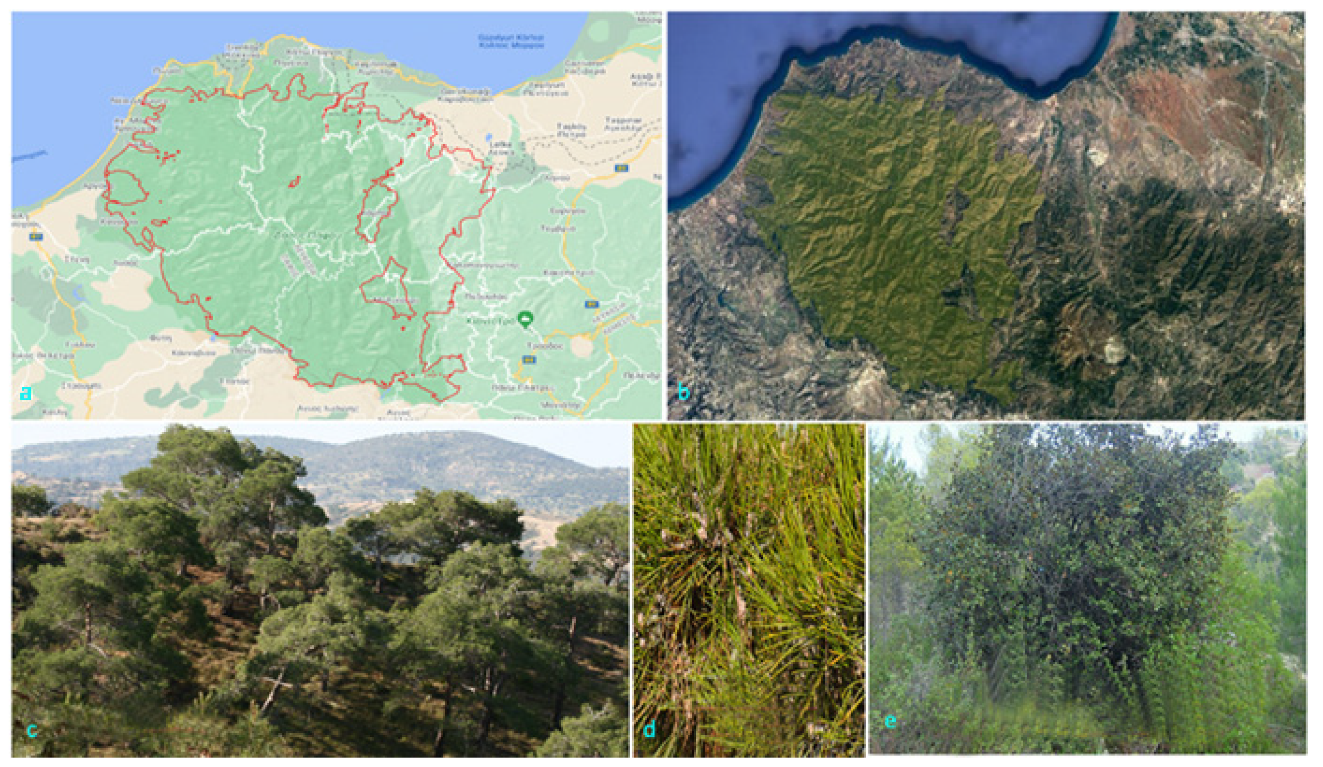
2. Study Area
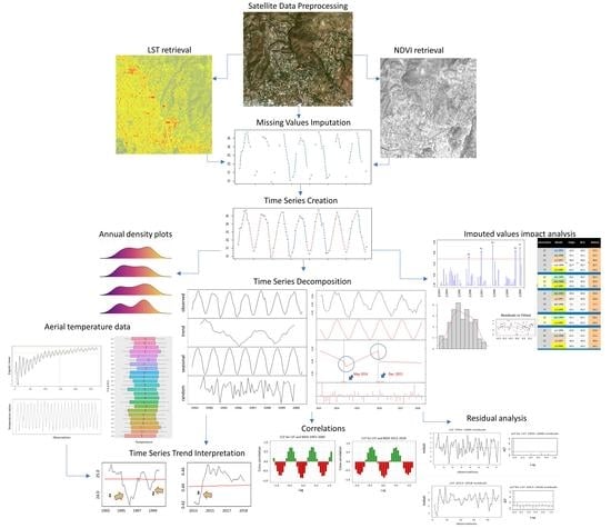
3. Materials and Methods
3.1. Data
3.2. Methods
4. Results and Discussion
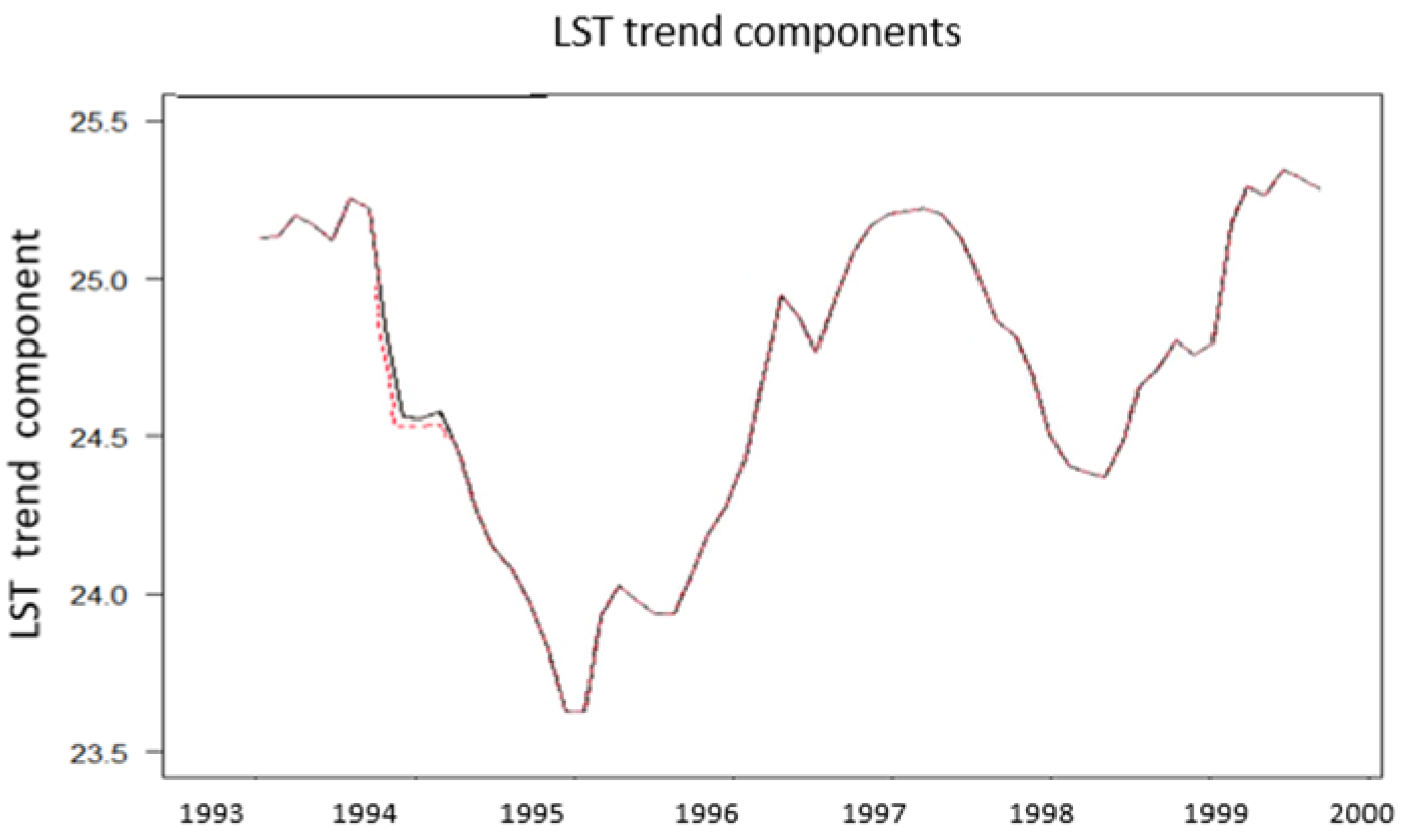
4.1. The Effect of Missing Values in the Satellite Time Series
4.2. Annual Density Plots and First Order Statistics
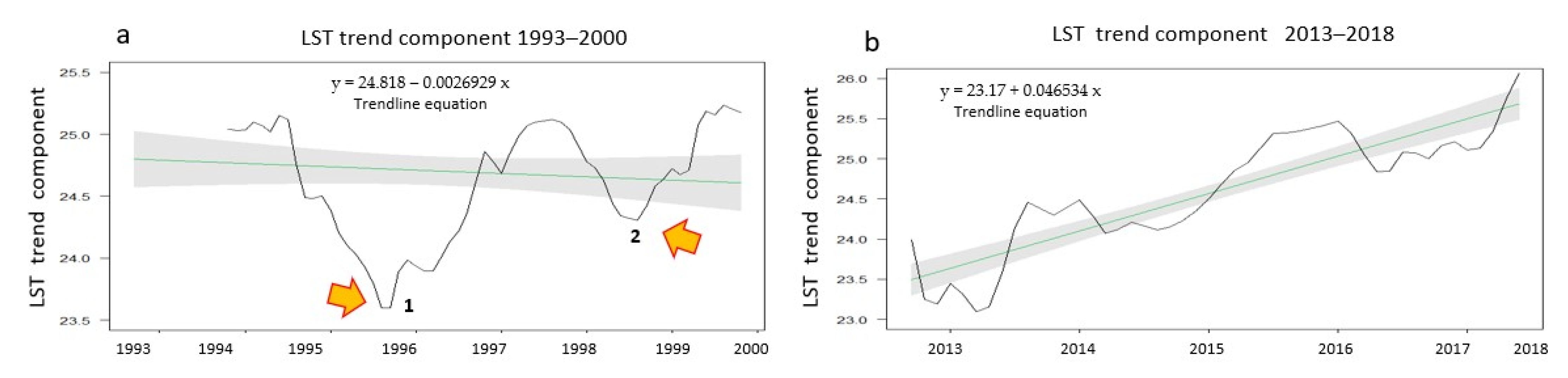
4.3. Remarks on Time Series Trends
4.3.1. Aerial temperature
4.3.2. LST
4.3.3. NDVI
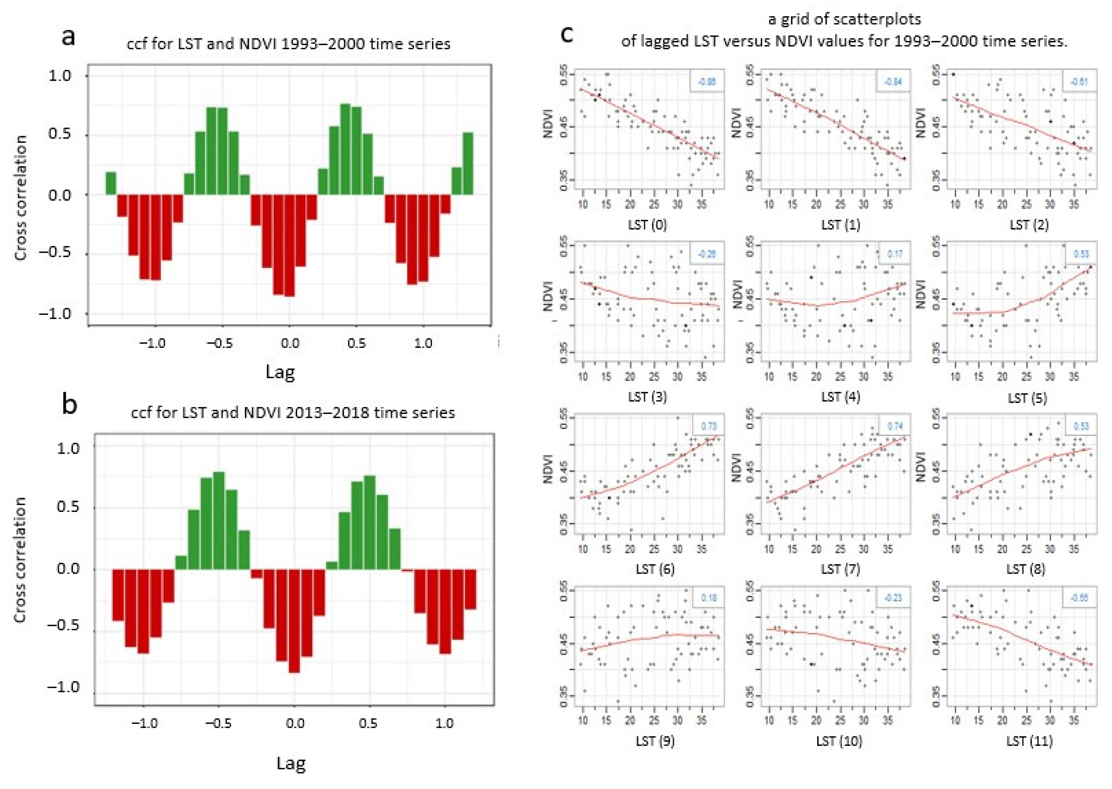
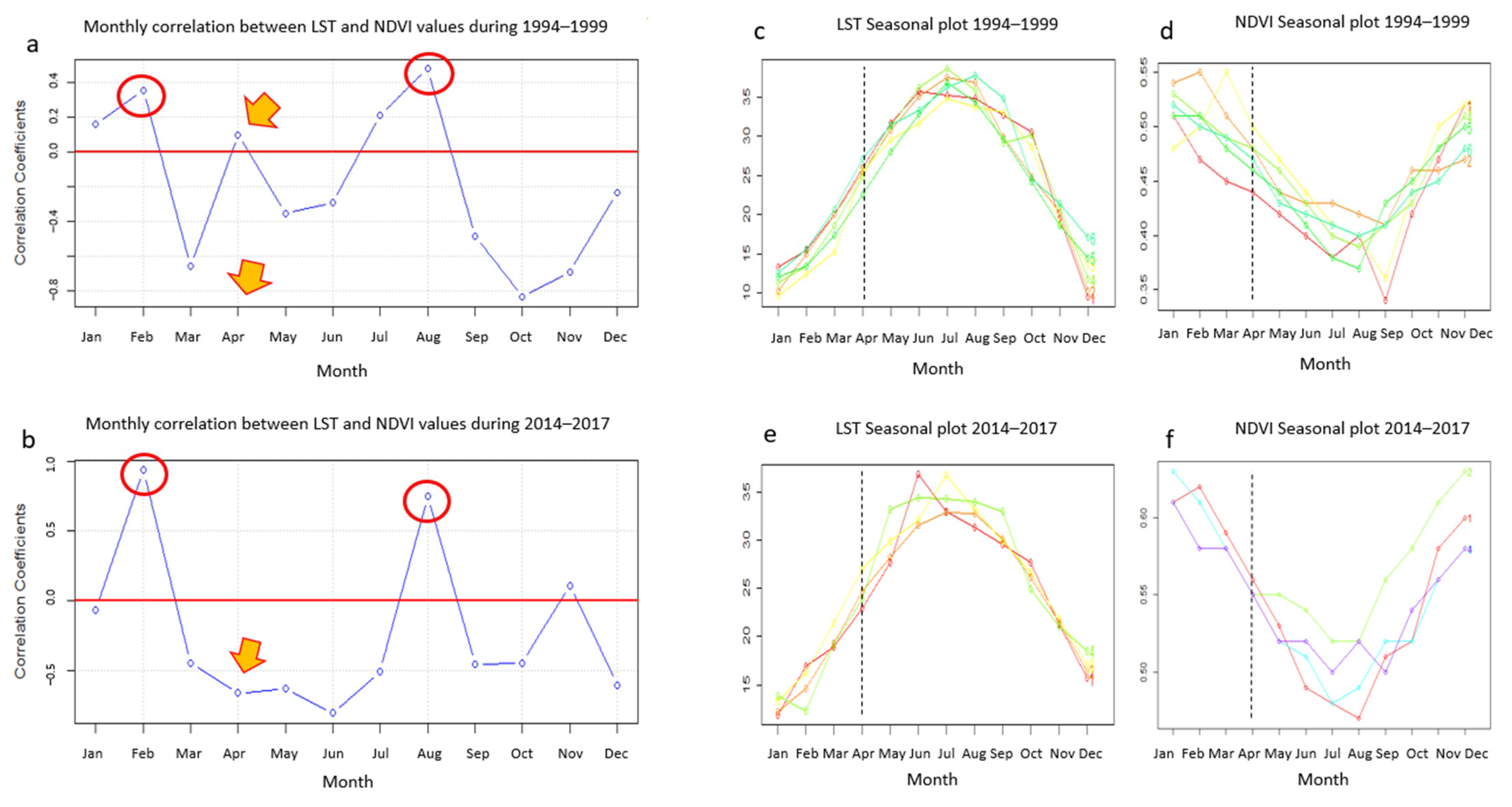
4.4. LST and NDVI Correlations
4.5. Analysis of the Residuals
4.6. Computational Requirements and Limitations
5. Conclusions
Author Contributions
Funding
Data Availability Statement
Acknowledgments
Conflicts of Interest
References
- Solanky, V.; Singh, S.; Katiyar, S.K. Land Surface Temperature Estimation Using Remote Sensing Data. In Hydrologic Modeling; Springer: Singapore, 2018. [Google Scholar]
- Dash, P. Land Surface Temperature and Emissivity Retrieval from Satellite Measurements; Forschungszentrum Karlsruhe: Karlsruhe, Germany, 2005; pp. 1–99. [Google Scholar]
- Yang, J.; Ren, J.; Sun, D.; Xiao, X.; Xia, J.; Jin, C.; Li, X. Understanding land surface temperature impact factors based on local climate zones. Sustain. Cities Soc. 2021, 69, 102818. [Google Scholar] [CrossRef]
- Ali, S.B.; Patnaik, S.; Madguni, O. Microclimate land surface temperatures across urban land use/ land cover forms. Glob. J. Environ. Sci. Manag. 2017, 3, 231–242. [Google Scholar] [CrossRef]
- Rajendran, P.; Mani, D.K. Estimation of Spatial Variability of Land Surface Temperature using Landsat 8 Imagery. Int. J. Eng. Sci. 2015, 4, 19–23. [Google Scholar]
- Han, H.; Bai, J.; Ma, G.; Yan, J. Vegetation phenological changes in multiple landforms and responses to climate change. ISPRS Int. J. Geo-Inf. 2020, 9, 111. [Google Scholar] [CrossRef] [Green Version]
- Yan, Y.; Mao, K.; Shi, J.; Piao, S.; Shen, X.; Dozier, J.; Liu, Y.; Ren, H.L.; Bao, Q. Driving forces of land surface temperature anomalous changes in North America in 2002–2018. Sci. Rep. 2020, 10, 6931. [Google Scholar] [CrossRef]
- Akinyemi, F.O.; Ikanyeng, M.; Muro, J. Land cover change effects on land surface temperature trends in an African urbanizing dryland region. City Environ. Interact. 2019, 4, 100029. [Google Scholar] [CrossRef]
- Dang, T.; Yue, P.; Bachofer, F.; Wang, M.; Zhang, M. Monitoring land surface temperature change with landsat images during dry seasons in Bac Binh, Vietnam. Remote Sens. 2020, 12, 4067. [Google Scholar] [CrossRef]
- Heinemann, S.; Siegmann, B.; Thonfeld, F.; Muro, J.; Jedmowski, C.; Kemna, A.; Kraska, T.; Muller, O.; Schultz, J.; Udelhoven, T.; et al. Land surface temperature retrieval for agricultural areas using a novel UAV platform equipped with a thermal infrared and multispectral sensor. Remote Sens. 2020, 12, 1075. [Google Scholar] [CrossRef] [Green Version]
- How, D.; Aik, J.; Ismail, M.H.; Muharam, F.M. Land Use/Land Cover Changes and the Relationship. Land 2020, 9, 372. [Google Scholar]
- Lambin, E.F.; Ehrlich, D. The surface temperature-vegetation index space for land cover and land-cover change analysis. Int. J. Remote Sens. 1996, 17, 463–487. [Google Scholar] [CrossRef]
- Mohd Jaafar, W.S.W.; Maulud, K.N.A.; Muhmad Kamarulzaman, A.M.; Raihan, A.; Sah, S.M.; Ahmad, A.; Maizah Saad, S.N.; Mohd Azmi, A.T.; Syukri, N.K.A.J.; Khan, W.R. The influence of deforestation on land surface temperature-A case study of Perak and Kedah, Malaysia. Forests 2020, 11, 670. [Google Scholar] [CrossRef]
- Rodrigues, C.; Teodoro, A.C.M. Relationship between the land surface temperature and the vegetation proportion to identify Heat Islands. Case study of Brasília (Brazil). In Proceedings of the Earth Resources and Environmental Remote Sensing/GIS Applications XI, Online, 21–25 September 2020; Schulz, K., Nikolakopoulos, K.G., Michel, U., Eds.; SPIE: Bellingham, WA, USA, 2020; p. 34. Available online: https://www.spiedigitallibrary.org/conference-proceedings-of-spie/11534/1153411/Relationship-between-the-land-surface-temperature-and-the-vegetation-proportion/10.1117/12.2572802.short?SSO=1 (accessed on 31 January 2022). [CrossRef]
- Guha, S.; Govil, H. An assessment on the relationship between land surface temperature and normalized difference vegetation index. Environ. Dev. Sustain. 2021, 23, 1944–1963. [Google Scholar] [CrossRef]
- Tang, B.; Zhao, X.; Zhao, W. Local effects of forests on temperatures across Europe. Remote Sens. 2018, 10, 529. [Google Scholar] [CrossRef] [Green Version]
- Macarof, P.; Groza, S.; Statescu, F. Investiganting Correlation LST and Vegetation Indices Using Landsat Images for the Warmest Month: A Case Study of Iasi County. Ann. Valahia Univ. Targoviste, Geogr. Ser. 2018, 18, 33–40. [Google Scholar] [CrossRef] [Green Version]
- Liu, Y.; Yamaguchi, Y.; Ke, C. Reducing the discrepancy between ASTER and MODIS land surface temperature products. Sensors 2007, 7, 3043–3057. [Google Scholar] [CrossRef] [PubMed] [Green Version]
- Meng, X.; Cheng, J.; Zhao, S.; Liu, S.; Yao, Y. Estimating land surface temperature from Landsat-8 data using the NOAA JPSS enterprise algorithm. Remote Sens. 2019, 11, 155. [Google Scholar] [CrossRef] [Green Version]
- Abdul Athick, A.S.M.; Shankar, K.; Naqvi, H.R. Data on time series analysis of land surface temperature variation in response to vegetation indices in twelve Wereda of Ethiopia using mono window, split window algorithm and spectral radiance model. Data Br. 2019, 27, 104773. [Google Scholar] [CrossRef] [PubMed]
- Quan, J.; Zhan, W.; Chen, Y.; Wang, M.; Wang, J. Time series decomposition of remotely sensed land surface temperature and investigation of trens and seasonal variations in surface urban heat islands. Nature 1955, 175, 238. [Google Scholar] [CrossRef]
- Qiu, S.; Zhu, Z.; He, B. Fmask 4.0: Improved cloud and cloud shadow detection in Landsats 4–8 and Sentinel-2 imagery. Remote Sens. Environ. 2019, 231, 111205. [Google Scholar] [CrossRef]
- Saputra, M.D.; Hadi, A.F.; Riski, A.; Anggraeni, D. Handling Missing Values and Unusual Observations in Statistical Downscaling Using Kalman Filter. J. Phys. Conf. Ser. 2021, 1863, 012035. [Google Scholar] [CrossRef]
- Muflihah Rizky Yudha Pahlawan Perbandingan Teknik Interpolasi Berbasis R Dalam Estimasi Data Curah Hujan Bulanan Yang Hilang Di Sulawesi Comparison of R-Based Interpolation Techniques To Estimate. 2017, pp. 107–111. Available online: http://puslitbang.bmkg.go.id/jmg/index.php/jmg/article/download/343/pdf (accessed on 17 February 2022).
- Welch, G.; Bishop, G. An Introduction to the Kalman Filter; ACM, Inc.: Tipp City, OH, USA, 2001. [Google Scholar]
- Kumar, D.; Shekhar, S. Statistical analysis of land surface temperature-vegetation indexes relationship through thermal remote sensing. Ecotoxicol. Environ. Saf. 2015, 121, 39–44. [Google Scholar] [CrossRef] [PubMed]
- Potter, C.; Coppernoll-Houston, D. Controls on land surface temperature in deserts of southern california derived from MODIS satellite time series analysis, 2000 to 2018. Climate 2019, 7, 32. [Google Scholar] [CrossRef] [Green Version]
- Lambert, J.; Drenou, C.; Denux, J.P.; Balent, G.; Cheret, V. Monitoring forest decline through remote sensing time series analysis. GIScience Remote Sens. 2013, 50, 437–457. [Google Scholar] [CrossRef]
- Ben Abbes, A.; Bounouh, O.; Farah, I.R.; de Jong, R.; Martínez, B. Comparative study of three satellite image time-series decomposition methods for vegetation change detection. Eur. J. Remote Sens. 2018, 51, 607–615. [Google Scholar] [CrossRef] [Green Version]
- Schelter, B.; Winterhalder, M. Handbook of Time Series Analysis; Wiley-VCH: Berlin, Germany, 2006; ISBN 9780471363552. [Google Scholar]
- Dagum, E.B. Time Series Modeling and Decomposition. Statistica 2010, 70, 433–457. [Google Scholar] [CrossRef]
- Sutcliffe, A. X11 Time Series Decomposition and Sampling Errors; Australian Bureau of Statistics: Melbourne, Australia, 1993.
- Cleveland, W.R.; Cleveland, J.; McRae, I.T. Statistics Sweden. J. Off. Stat. 1990, 6, 3–73. [Google Scholar]
- Verbesselt, J.; Hyndman, R.; Zeileis, A.; Culvenor, D. Phenological Change Detection While Accounting for Abrupt and Gradual Trends in Satellite Image Time Series. Remote Sens. Environ. 2010, 114, 2970–2980. [Google Scholar] [CrossRef] [Green Version]
- Rhif, M.; Ben Abbes, A.; Martinez, B.; Farah, I.R. An improved trend vegetation analysis for non-stationary NDVI time series based on wavelet transform. Environ. Sci. Pollut. Res. 2020, 28, 46603–46613. [Google Scholar] [CrossRef]
- Zachariadis, T. Climate Change in Cyprus: Impacts and Adaptation Policies. Cyprus Econ. Policy Rev. 2012, 16, 21–37. [Google Scholar]
- Miltiadou, M.; Antoniou, E.; Theocharidis, C.; Danezis, C. Do people understand and observe the effects of climate crisis on forests? The case study of cyprus. Forests 2021, 12, 1152. [Google Scholar] [CrossRef]
- Republic of Cyprus, Ministry of Agriculture; N.R. and E. Paphos Forest Management Plan: Nicosia, Cyprus, 2011.
- Hansen, M.C.; Potapov, P.V.; Moore, R.; Hancher, M.; Turubanova, S.A.; Tyukavina, A.; Thau, D.; Stehman, S.V.; Goetz, S.J.; Loveland, T.R.; et al. University of M. High-Resolution Global Maps of 21st-Century Forest Cover Change. Science 2013, 342, 850–853. [Google Scholar] [CrossRef] [PubMed] [Green Version]
- Jennings, R.C. The locust problem in cyprus. Bull. Sch. Orient. African Stud. 1988, 51, 279–313. [Google Scholar] [CrossRef]
- Hódar, J.A.; Castro, J.; Zamora, R. Pine processionary caterpillar Thaumetopoea pityocampa as a new threat for relict Mediterranean Scots pine forests under climatic warming. Biol. Conserv. 2003, 110, 123–129. [Google Scholar] [CrossRef]
- Invasive Species Compendium Thaumetopoea Pityocampa (Pine Processionary). Available online: https://www.cabi.org/isc/datasheet/53501#toenvironments (accessed on 2 February 2022).
- SOER Country Profile—Distinguishing Factors (Cyprus). Available online: https://www.eea.europa.eu/soer/2010/countries/cy/country-introduction-cyprus (accessed on 31 January 2022).
- Moritz, S.; Bartz-Beielstein, T. ImputeTS: Time series missing value imputation in R. R J. 2017, 9, 207–218. [Google Scholar] [CrossRef] [Green Version]
- Dennis Cook, S.W. Residuals and Influence in Regression; Chapman and Hall: New York, NY, USA, 1982. [Google Scholar]
- Hilas, C.S.; Goudos, S.K.; Sahalos, J.N. Seasonal decomposition and forecasting of telecommunication data: A comparative case study. Technol. Forecast. Soc. Change 2006, 73, 495–509. [Google Scholar] [CrossRef]
- Mutiibwa, D.; Strachan, S.; Albright, T. Land Surface Temperature and Surface Air Temperature in Complex Terrain. IEEE J. Sel. Top. Appl. Earth Obs. Remote Sens. 2015, 8, 4762–4774. [Google Scholar] [CrossRef]
- Xu, D. Compare NDVI Extracted from Landsat 8 Imagery with that from Landsat 7 Imagery. Am. J. Remote Sens. 2014, 2, 10. [Google Scholar] [CrossRef] [Green Version]
- Vogelmann, J.E.; Helder, D.; Morfitt, R.; Choate, M.J.; Merchant, J.W.; Bulley, H. Effects of Landsat 5 Thematic Mapper and Landsat 7 Enhanced Thematic Mapper plus radiometric and geometric calibrations and corrections on landscape characterization. Remote Sens. Environ. 2001, 78, 55–70. [Google Scholar] [CrossRef] [Green Version]
- Schachat, S.R.; Labandeira, C.C.; Maccracken, S.A. The importance of sampling standardization for comparisons of insect herbivory in deep time: A case study from the late palaeozoic. R. Soc. Open Sci. 2018, 5, 171991. [Google Scholar] [CrossRef] [Green Version]


| Time Series | Min. | 1st Quantile | Median | Mean | 3rd Quantile | Max. | Stdev |
|---|---|---|---|---|---|---|---|
| LST 1993–2000 | 8.40 | 18.38 | 25.50 | 24.89 | 32.25 | 36.80 | 7.722 |
| NDVI 1993–2000 | 0.34 | 0.41 | 0.45 | 0.45 | 0.49 | 0.55 | 0.049 |
| aerial 1993–2000 | 5.70 | 10.57 | 18.20 | 18.44 | 25.50 | 31.70 | 7.755 |
| LST 2013–2018 | 9.50 | 17.32 | 25.85 | 25.01 | 32.73 | 38.60 | 8.892 |
| NDVI 2013–2018 | 0.47 | 0.52 | 0.56 | 0.56 | 0.59 | 0.63 | 0.044 |
| aerial 2013–2016 | 7.30 | 13.10 | 19.05 | 19.00 | 24.43 | 30.10 | 7.108 |
Publisher’s Note: MDPI stays neutral with regard to jurisdictional claims in published maps and institutional affiliations. |
© 2022 by the authors. Licensee MDPI, Basel, Switzerland. This article is an open access article distributed under the terms and conditions of the Creative Commons Attribution (CC BY) license (https://creativecommons.org/licenses/by/4.0/).
Share and Cite
Andronis, V.; Karathanassi, V.; Tsalapati, V.; Kolokoussis, P.; Miltiadou, M.; Danezis, C. Time Series Analysis of Landsat Data for Investigating the Relationship between Land Surface Temperature and Forest Changes in Paphos Forest, Cyprus. Remote Sens. 2022, 14, 1010. https://0-doi-org.brum.beds.ac.uk/10.3390/rs14041010
Andronis V, Karathanassi V, Tsalapati V, Kolokoussis P, Miltiadou M, Danezis C. Time Series Analysis of Landsat Data for Investigating the Relationship between Land Surface Temperature and Forest Changes in Paphos Forest, Cyprus. Remote Sensing. 2022; 14(4):1010. https://0-doi-org.brum.beds.ac.uk/10.3390/rs14041010
Chicago/Turabian StyleAndronis, Vassilis, Vassilia Karathanassi, Victoria Tsalapati, Polychronis Kolokoussis, Milto Miltiadou, and Chistos Danezis. 2022. "Time Series Analysis of Landsat Data for Investigating the Relationship between Land Surface Temperature and Forest Changes in Paphos Forest, Cyprus" Remote Sensing 14, no. 4: 1010. https://0-doi-org.brum.beds.ac.uk/10.3390/rs14041010