Article

A Graph Convolutional Incorporating GRU Network for Landslide Displacement Forecasting Based on Spatiotemporal Analysis of GNSS Observations

1
College of Earth Science, Chengdu University of Technology, Chengdu 610059, China
2
State Key Laboratory of Geohazard Prevention and Geoenvironment Protection, Chengdu University of Technology, Chengdu 610059, China
3
Huffington Department of Earth Sciences, Southern Methodist University, Dallas, TX 75275, USA
4
Technology Service Center of Surveying and Mapping, Sichuan Bureau of Surveying, Mapping and Geoinformation, Chengdu 610081, China
5
School of Architecture and Civil Engineering, Chengdu University, Chengdu 610106, China
*
Author to whom correspondence should be addressed.
Submission received: 12 January 2022 / Revised: 12 February 2022 / Accepted: 14 February 2022 / Published: 19 February 2022
(This article belongs to the Special Issue GNSS, Space Weather and TEC Special Features)

Abstract

:
Landslide displacement prediction is crucial for the early warning of slope failure but remains a challenging task due to its spatiotemporal complexity. Although temporal dependency has been well studied and discussed, spatial dependence is relatively less explored due to its significant variations of the spatial structure of landslides. In this study, a novel graph convolutional incorporating GRU network (GC-GRU-N) is proposed and applied to landslide displacement forecasts. The model conducts attribute-augmented graph convolution (GC) operations on GNSS displacement data with weighted adjacency matrices and an attribute-augmented unit to combine features, including the displacements, the distance, and other external influence factors to capture spatial dependence. The output of multi-weight graph convolution is then applied to the gated recurrent unit (GRU) network to learn temporal dependencies. The related optimal hyper-parameters are determined by comparison experiments. When applied to two typical landslide sites in the Three Gorge Reservoir (TGR), China, GC-GRU-N outperformed the comparative models in both cases. The ablation experiment results also show that the attribute augmentation, which considers external factors of landslide displacement, can further improve the model’s prediction performance. We conclude that the GC-GRU-N model can provide robust landslide displacement forecasting with high efficiency.

1. Introduction

Landslides are a harmful environmental and geological phenomenon, occurring frequently worldwide [1,2]. They are gradually formed by the long-term interactions of both natural and human factors under specific geologic and geographic conditions. The occurrence of landslides is irreversible, and a severe landslide may induce a series of geological environmental disasters and form a disaster chain, posing severe threats to human life and built infrastructures [3]. Thus, analyzing and predicting geological hazards using monitoring data collected from various sources is essential to mitigate these severe devastations.
Time series landslide displacement, directly reflecting the deformation and stability of a slope, is the most critical dataset to understand landslide characteristics and infer its future development [4]. For instance, the Global Navigation Satellite System (GNSS), measuring surface motion at a very high frequency and accuracy, is a powerful tool to help diagnose the progression of landslide movement. For this reason, these datasets enable deep-learning models to be trained for predicting the future state of surface deformation.
Deep-learning approaches, as suggested, are superior to traditional statistical methods in many applications, especially in time-series prediction [5,6]. Representative statistical models, such as multivariate regression models (MLR) [7], auto-regressive integrated moving average (ARIMA) [8], and others, are widely used for a single time series forecasting [8,9,10,11,12], while they neglect the potential relationship among multiple time series in the monitoring network under similar geological conditions. By comparison, deep-learning methods integrate various processing layers and produce abstract learning features and nonlinear dependencies from multidimensional datasets [6,11,13], making them sound alternatives in landslide displacement forecasting.
Given the outstanding performance in time-series forecasts, recurrent neural networks (RNN) and their variants [14], such as long short-term memory (LSTM) and gated recurrent unit (GRU), have achieved impressive results in the prediction of land displacements based on GNSS time-series data [9,10]. These models can solve the problems of nonlinear dynamic characteristics in complex time series, thus being particularly suitable to predict time-series landslide displacement. The workflows of these methods are approximately the same: select representative GNSS monitoring stations and plot the curve of displacement–time to analyze the deformation; next, the monitoring data of specific stations will be adopted for modelling one station by one station; as each displacement–time curve only shows the evolution characteristics of a single monitoring point, the model predictions only reflect the displacement behaviour of a single location.
However, landslide-displacement prediction is a spatiotemporal task because the evolution of the landslide process often exhibits spatial and temporal characteristics. The existing time-series forecast model only explores temporal features, ignoring the underlying spatial correlations. Thus, it is difficult to comprehensively assess the displacement changes of the entire monitoring system and reveal the future state of the landslide as a whole. Several studies have utilized convolutional neural networks (CNNs) to explore the spatial dependencies and build prediction models in traffic forecasting problems [6,15,16,17]. However, CNN-based models only consider the absolute distance relationship among stations in Euclidean space. Compared with CNN, graph convolutional networks (GCNs) can handle neighbourhood information in non-Euclidean spaces, providing a more feasible way to model spatial dependencies within a monitoring network [13,17,18].
Based on the problems mentioned above and inspired by current encouraging results in traffic forecasting problems, there is a need to combine GCN and RNN models to build a collaborative prediction model to capture spatial and temporal features for spatial–temporal forecast problems. However, displacement prediction of a landslide relies not only on historical GNSS measurements and the spatial correlations of the monitoring network but also on internal geological conditions and various external factors, such as hydrologic conditions [19,20,21,22], anthropogenic factors, etc. For example, in China’s Three Gorges Reservoir area, many landslides are triggered and accelerated by seasonal precipitation and the fluctuation of reservoir water level [17,19]; thus, the impact factors in predicting landslide deformation are indispensable during modelling.
To the best of the authors’ knowledge, there is currently no related work focusing on addressing the prediction of rainfall reservoir-induced landslide displacement from a holistic perspective combining the external incentive factors. Inspired by current encouraging results in traffic forecasting problems [13,18], we propose a novel deep-learning method named graph convolutional incorporating gated recurrent unit network (GC-GRU-N). In the GC-GRU-N, the monitored GNSS time-series displacements, the distance, and other external triggering factors are integrated to construct the GCN module handling the spatial dependency; the GRU module model’s temporal dependence captures long-term dependencies by considering landslide displacement time series. This architecture is expected to inherit the merits from both GCN in extracting spatial dependencies and GRU in capturing temporal correlation features. The main contributions are twofold. First, we have extended GCN for spatial data imputation in the GNSS network deployed on the landslides. Second, we introduce a graph deep-learning framework to predict landslide displacement in time and space.

2. Methods

Landslide displacement forecasting is a spatiotemporal prediction task because the evolution of landslide movement often exhibits spatial and temporal characteristics. This paper proposes a deep-learning framework to predict the landslide displacement based on the spatiotemporal analysis of the time series monitoring data. This framework is expected to inherit the merits from both GCN in extracting spatial dependencies and GRU in capturing temporal correlation features.
The workflow is shown in Figure 1. According to the GNSS monitoring network structure and the obtained time-series datasets, pro-processing is conducted to obtain spatial and temporal attributes as the model inputs. Then, the GCN module is employed to handle spatial dependencies, while the GRU module is used to capture temporal dependencies. This paper uses tensorFlow2.1, Python3.6, and Matlab2020 to conduct the experiments and analysis.

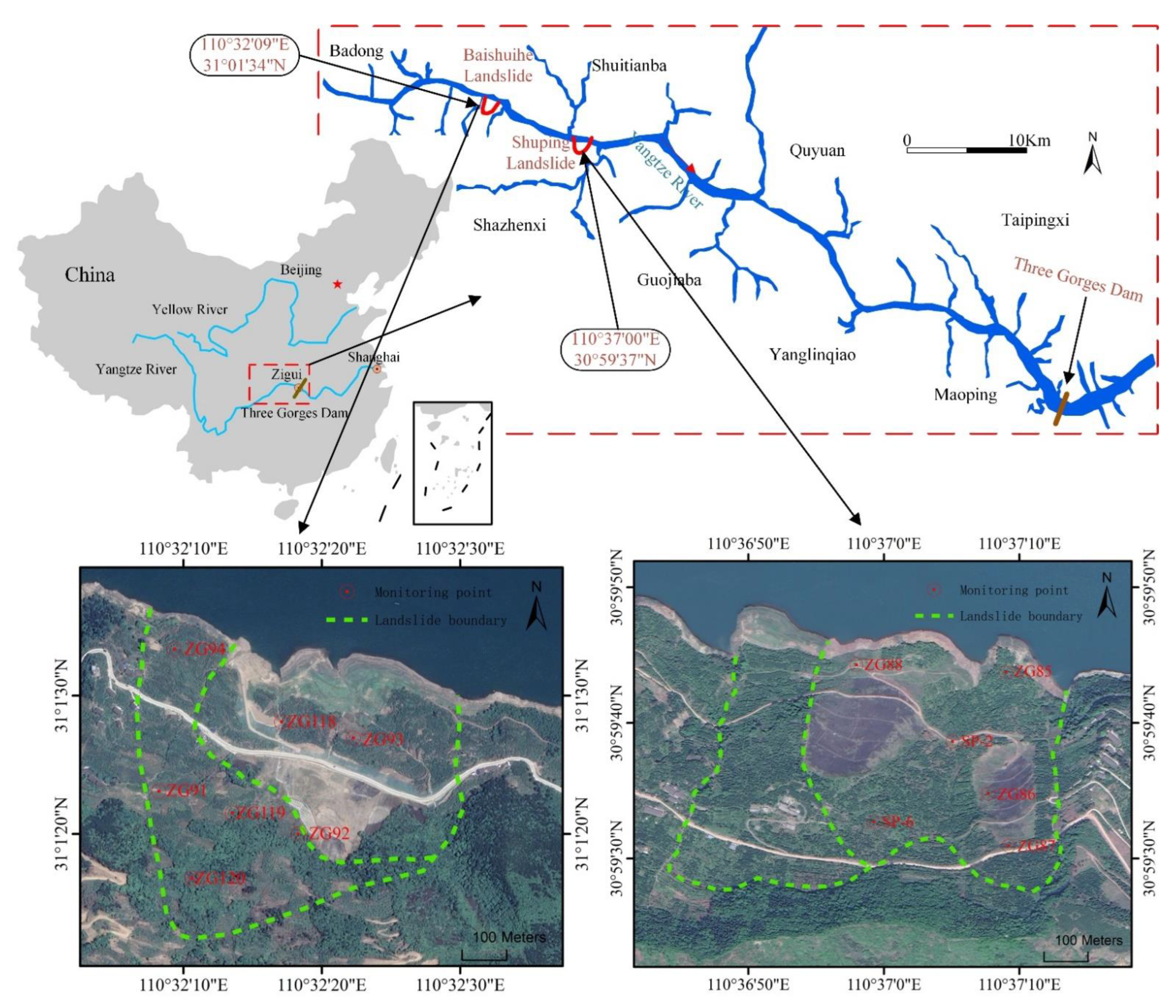
2.1. Study Area and Dataset

Since the Three Gorges Reservoir (TGR) was used in 2003, the fluctuated water level has changed the rock and soil physical and mechanical properties around the reservoir [19]. Over 4200 landslides are distributed in this region, and the majority of these landslides show characteristics of multiple triggers and reactivations [4]. The Baishuihe landslide and the Shuping landslide (Figure 2) are two typical recurrence reservoir landslides that have attracted the concern of researchers for a long time. As shown in Figure 2, both landslides are located on the south bank of the Yangtze River and spread into the Yangtze River.
The Shuping landslide has an elevation of between 65 m and 400 m and is about 650 m wide. It is a south–north-oriented slope with a gradient varying from 22° in the upper part to 35° in the lower part. The overall sliding mass is about 27 million m3 with a thickness of approximately 40–70 m [19]. According to the field investigation, this landslide is divided by a valley into two blocks (Figure 2).
While the maximal dimensions of the Baishui landslide in the north–south and east–west are 780 m and 700 m, respectively, it has a volume of about 12.6 million m3 with an average thickness of approximately 30 m [20]. The field investigation and monitoring data have confirmed that the landslide has a relatively flat central part with more significant gradients in the upper and lower parts of the landslide. It can also be categorized as two blocks (Figure 2).
The two landslides were re-activated by the first impoundment of the TGR, and since then, visible cracks have gradually formed [19,20]. Two GNSS networks were deployed to study the displacement characteristics during landslide evolution (Figure 2). The displacement dataset was collected monthly by the Trimble GPS receiver with a plane accuracy of 5 ± 1 ppm. The measurements of the reservoir water level were collected daily by the water level indicator provided by the China Three Gorges Project Development Corporation. The precipitation observations were collected daily by the rain gauge provided by Zigui County Meteorological Bureau. These collected datasets (from July 2003 to March 2013 for the Baishuihe landslide; from September 2007 to May 2015 for the Shuping landslide) are presented in Figure 3 and Figure 4. It can be inferred from Figure 3 and Figure 4 that:
(1)
The TGR became fully operational in November 2008 when its highest water level reached 175 m. Since then, the reservoir water level has fluctuated between 145 m and 175 m in a year, exhibiting seasonal changes due to artificial flood control.
(2)
The rainy season of the study area lasts from June to October each year. The rainfall data also display seasonal variations due to monsoon influences. In contrast, the reservoir began impounding at the end of the wet season in October and quickly reached the maximum water level and maintained this from November to February, with a cycle opposite to the precipitation conditions.
(3)
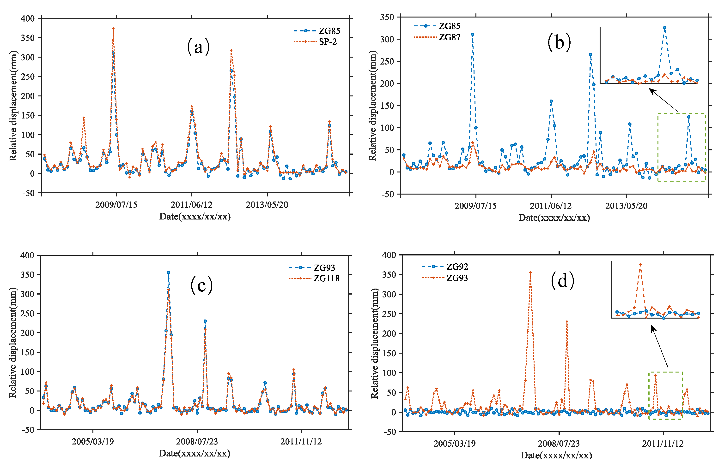
The historical GNSS measurements of both landslides also show evident seasonal patterns. The displacements increase from April to September per year and remain relatively stable from October to April in the next subsequent year. The displacements rise with the drawdown of the reservoir water level and during the period of increased rainfall in the wet season.
Thus, the seasonal characteristics of the evolution of the landslides are a joint effort of the precipitation and the fluctuation of reservoir water levels, with a period of about a year.

2.2. Data Processing

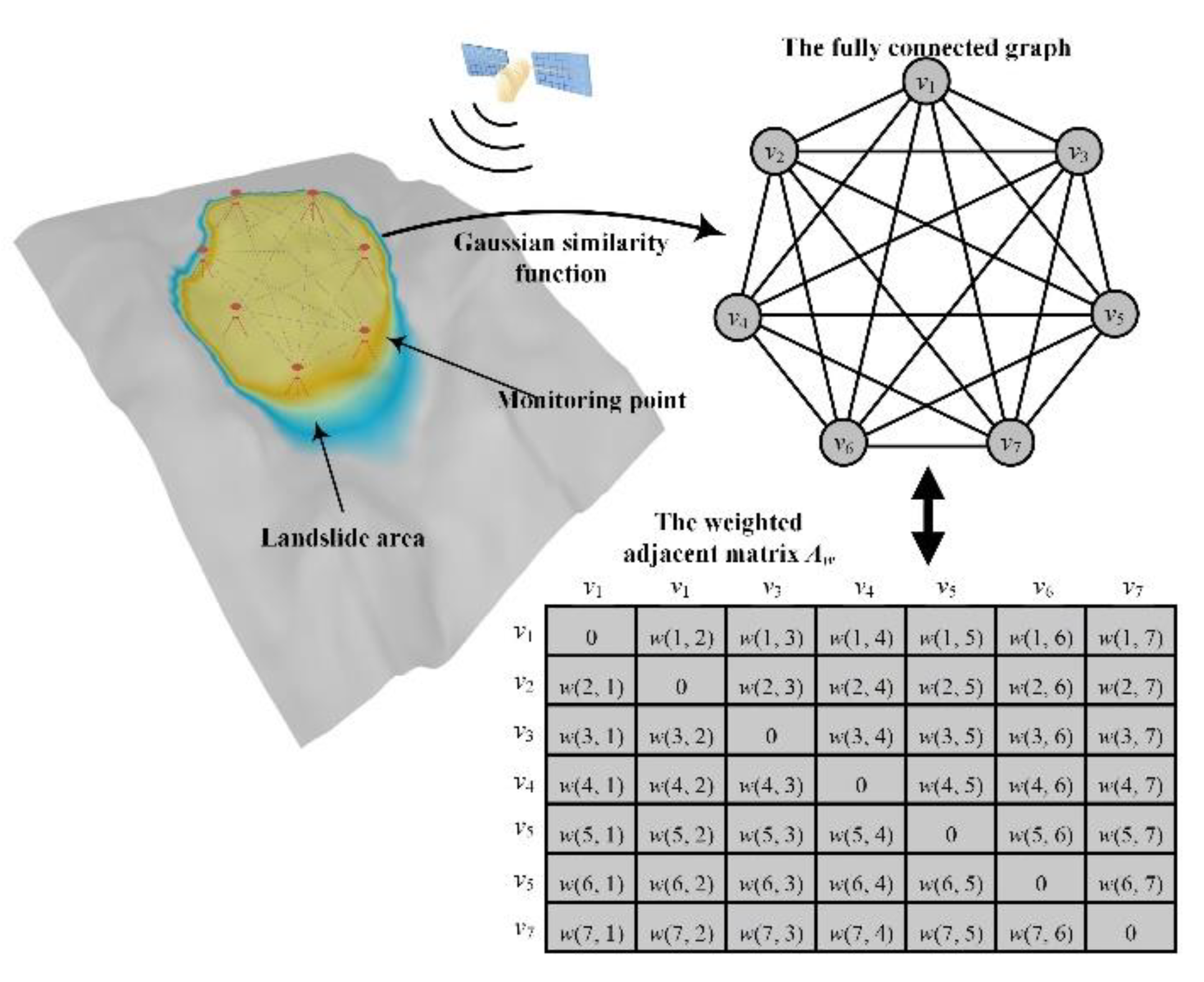
2.2.1. Representation of the Spatial Correlation

Our framework defines the GNSS monitoring network structure as a weighted graph G = (V, E, W). The monitoring sites are regarded as nodes, symbolized by V, and E is a finite set of edges representing the connection between the nodes. The numbers of the edges are N(N − 1)/2, where N is the number of monitoring stations of the network, WRN×N is a weighted adjacency matrix representing the correlation between the nodes (Figure 5).
Generally, the deformation characteristics of a landslide at different parts vary with the monitoring site’s location. The spatial correlation of monitoring sites in the GNSS network graph shows a strong place dependence. Thus, the weighted adjacency matrix is calculated using the Gaussian similarity functions based on spatial proximity. As given in Equation (1), weights wij of edges eij representing the spatial correlation between nodes (vi, vj) can be calculated.
w ( i , j ) = exp ( v i v j 2 / 2 σ 2 )
where v i v j 2 denotes the spatial dependence between nodes (vi, vj), and σ is the standard deviation controlling the width of the neighbourhoods.
The weighted adjacency matrix can be expressed as Equation (2), where a more significant weight indicates a higher correlation between the two neighbourhood nodes.
A w = ( 0 w ( 1 , 2 ) w ( 1 , N ) w ( 2 , 1 ) 0 w ( 2 , N ) w ( N , 1 ) w ( N , 2 ) 0 )

2.2.2. Representation of the Temporal Correlation

The spatial and temporal attributes are two critical elements of landslide displacement prediction. This section will explore the node features that can represent the temporal correlation. Once the displacement data are collected through the GNSS monitoring system, preprocessing is needed before analysis. Outlier removal and missing value imputation are first carried out, followed by denoising and normalization. This study applies a wavelet-based denoising method to remove the random noise and improve the data quality. Then, the monitoring date is normalized into the range from 0 to 1 by max-min normalization to eliminate dimensional effects.
A feature matrix XRN×P is defined, which contains the time-series information of the monitoring stations (nodes). Where N is the number of monitoring stations in the network, P denotes the number of node time-series features, such as the length of the historical time series. XRN×t represents the displacement at each monitoring station at time t. Thus, the input [Xt-n, …, Xt−1, Xt] is a sequence of n historical displacement dataset, and [Xt+1, …, Xt+T] is the predicted displacement in the following T time series.

2.2.3. Attribute Augmentation by Incorporating External Factors

Generally, the dynamic movement of a landslide is subject to internal geological conditions and external triggering factors [4,21]. As for landslides on the reservoir bank of TGR, the fluctuation of the reservoir water level and varying precipitation are two main external factors influencing landslide behaviours [22,23]. However, the studies using GCN to learn spatial dependencies often adhere to a single measure (e.g., distance) to represent the weights in the adjacency matrix [24,25] without considering the effects of the external trigging factors, which inevitably hampers the model performance given the complexity of landslide deformation patterns.
In this study, we apply attribute-augmented graph convolution operations on GNSS observations. The attribute-augmented unit integrates features of the displacements time series, the synchronous precipitation and the water level fluctuation to represent the contribution of the external dynamic triggering factors. The augmented matrix with weighted adjacency matrices is incorporated into the forecast model to enhance the extraction of realistic spatiotemporal dependency.
An attribute matrix DRN×(kt) stands for k external factors at time t. It considers that the effects of the triggering factors on the landslide displacements show significant time lags. We use an extended time window m + 1 to express the attribute information instead of the original one at time t; that is, the attribute matrix Dk is denoted by D t m , t k = [ D t m k , D t m 1 k , , D t k ] . Then, the attribute-augmented matrix S can be inferred by combining the feature matrix X and the attribute matrix D:
S t = [ X t , D t m , t 1 , D t m , t 2 , , D t m , t k ]
Thus, the displacement prediction task can be regarded as learning the function f to predict the displacements, as shown in Equation (4):
f ( G , X | D ) = [ X t + 1 , , X t + T ]

2.3. Data Modelling

2.3.1. Spatial Dependence Modeling by GCN

Acquiring complex spatial dependence is one of the critical problems in spatiotemporal predicting. Traditional CNN-based models can capture local spatial features but are only usable in Euclidean space, such as a regular grid [15]. The GNSS monitoring network deployed on a landslide is a graph structure rather than a two-dimensional grid, which means the traditional CNN cannot capture the spatial dependence correctly.
Recently, the GCN model has received widespread attention, extending convolutional operations to non-Euclidean domains. It has been gradually applied in image classification and traffic road networks and has demonstrated that the spatial structure captured by GCNs improves the forecasting accuracy [26].
Given an adjacency matrix A and a feature matrix X, the GCN model builds a filter to handle specific spectral information in the Fourier domain. The filter, working on the nodes (e.g., monitoring sites) of a graph (e.g., GNSS network structure), focuses on the nodes’ spatial features and measures their closeness by its first-order neighbourhood.
The GCN model learns the topological relationship between the nodes and their surrounding nodes for each node. Then, the encoder generates the latent representations for all geographical units of the monitoring network and the attributes of the nodes with graph convolution to obtain spatial dependence. As a result, similar units obtain similar representations, which are then used by the decoder for predicting.
As shown in Figure 6a, the GCN model can be constructed by stacking multiple convolutional layers to learn higher-order similarities between the nodes in the graph. The propagation of the GCN can be formulated as:
y l + 1 = σ ( D ˜ 1 2 A ˜ D ˜ 1 2 y l W l )
where σ(.) represents the nonlinear sigmoid function, such as the ReLU. A ˜ = A + I is a self-connection structure matrix with an identity matrix I. D ˜ is the diagonal node degree matrix of A ˜ , represents as D ˜ = j A ˜ i j . Wl is a weight matrix for the l-th neural network layer. yl is a node-level output of l layer with y0 = X.

2.3.2. Temporal Dependence Model by GRU

Acquiring temporal dependence is another crucial problem in landslide displacement spatiotemporal predicting. The recurrent neural network (RNN) has achieved impressive results given the outstanding time series forecasts [14]. However, traditional RNN has limitations for long-term forecasts due to deficiencies, such as gradient disappearance and explosion [27].
The LSTM model [28] and the GRU model [29] are proposed to address these problems. The basic principles of LSTM and GRU are almost identical. They all incorporate gated mechanisms and can handle longer sequences of tasks. Compared to LSTM, GRU combines the forget gate and the input gate into an update gate, decreasing the data flow; thus, it has a more straightforward structure, fewer parameters, and faster convergence speed [30]. Therefore, we have chosen the GRU model to learn temporal dependence from the displacement time series data.
The data flow of the GRU is illustrated in Figure 6b. xt denotes the model inputs at time t, ht−1 is the hidden state at time t − 1, all the subscript letter indicates time, rt stands for the reset gate, ut represents the update gate, ct is the memory content stored, and ht denotes the output state. The update gate ut is used to control the degree of the status information transmission from time t − 1 to time t; the larger the value of ut, the more critical the previous state. The reset gate tensor rt controls the influence of time t − 1 on-time t; the smaller the value of rt, the weaker the effect.
The GRU obtains the monitoring information at time t, by taking the hidden status at time t − 1 and the current monitoring information while capturing the monitoring information at the present moment; the model still retains the changing trend of historical monitoring information and can capture temporal dependence.

2.3.3. Spatiotemporal Model Using GC-GRU-N

To capture both spatial and temporal features from landslide monitoring data, we propose a new deep learning model (GC-GRU-N) based on graph convolutional network (GRU) and gated recurrent unit (GRU). In the model, an attribute-augmented graph convolution operation with weighted adjacency matrices and an attribute-augmented unit is employed to represent the spatiotemporal correlations of the monitoring network, and the obtained results will be used as the model inputs.
The architecture of the model is shown in Figure 7. The upper part shows the process of spatiotemporal displacement prediction. The GCN module is used to model spatial dependencies, while the GRU module is used to model temporal dependencies. A fusion layer is implemented to incorporate extracted features from both space- and time-domain. The model predicted displacement could be represented as f ( A , S ) with A the weighted adjacency matrix and S the attribute-augmented matrix.
The lower part (marked by a dashed box) gives a specific structure of a T-GCN cell. In each model cell, ht−1 denotes the output at time t − 1, gc(.) is the graph convolution process, ut, rt are the update gate and reset gate at time t, and ht denotes the output at time t. The calculation process of spatiotemporal displacement prediction is shown below:
u t = σ ( W u [ g c ( S t , A ) , h t 1 ] + b u )
r t = σ ( W r [ g c ( S t , A ) , h t 1 ] + b r )
c t = tanh ( W c [ g c ( S t , A ) , ( r t h t 1 ) ] + b c )
h t = u t h t 1 + ( 1 u t ) c t
where σ(.) and tanh(.) represents the sigmoid function, W and b stand for the weights and biases in the training process, respectively. * denotes the matrix multiplication.

2.3.4. Evaluation Metrics of the Prediction

To evaluate the model performance, we introduce three evaluation indicators, namely the mean absolute error (MAE), the mean absolute scaled error (MASE), and the root mean square error (RMSE) [31]. These metrics are widely used in the regression tasks, defined as follows:
M A E = 1 n t = 1 n | Y t Y ^ t |
M A S E = m e a n ( | e j 1 n 1 t = 2 n | Y t Y t 1 | | )
R M S E = 1 n t = 1 n ( Y t Y ^ t ) 2
where n is the length of time series, Y t represents the actual measurement, Y ^ t denotes the predicted value, and e j = t = 1 n | Y t Y ^ t | indicates the forecast error for a given period j (the number of forecasts). MAE can reflect the absolute error of the prediction result. MASE is a favourable property to calculate the time-series forecast errors, which can be used to compare forecasts across data sets with different scales. RMSE can more accurately reflect the similarity between the predicted and the observed sequence.

3. Experiments and Results

3.1. Analysis of the Spatiotemporal Correlation

Generally, the deformation of a landslide varies spatially at different parts of the landslide body (e.g., [19,20]). The spatial–temporal correlation of each monitoring site in the GNSS network shows a strong location dependence. This section analyzes the measurements on each monitoring site to determine their spatiotemporal relations. To do so, we introduce grey relational analysis (GRA) to help estimate the correlation of monitoring points [19]; it is believed that the value of grey relational degree (GRD) greater than 0.6 denotes a close correlation.
For the Shuping landslide, all monitoring stations (Figure 2) are deployed on the active block. As shown in Table 1, for any neighbouring connection, their GRD values are greater than 0.6, implying a strong spatial–temporal correlation among them. We select two pairs of adjacent monitoring points (ZG85 with SP-2 and ZG85 with ZG87) and plot the observed deformation time series. The results are illustrated in Figure 8a,b, showing the strong consistency of each pair. The calculated GRD value is 0.8 and 0.87, respectively, suggesting a strong spatiotemporal correlation between them. From these GNSS observations on the east block (Figure 2 and Figure 4), the landslide deforms locally obviously, indicting an unstable state. Still, it does not mean that the whole landslide is moving, or that the landslide is likely to occur, unless it is already entering an accelerated deformation stage with an increasingly accelerated velocity.
For the Baishuihe landslide, two stations, namely ZG93 and ZG118, are installed in the more active block, with the rest monitoring stations at the other block (Figure 2). It can be seen from Figure 2 and Figure 8c that monitoring sites located at the more active block exhibit almost identical displacement trends (GRD = 0.74). At the other monitoring sites in another block, the measured displacements are relatively small, fluctuating to within 20 mm per month. The GRD between these sites is larger than 0.6, reflecting remarkable similarity in displacement trends. Generally, the correlation decreases with increasing distance. However, for stations located at different blocks (e.g., ZG92 and ZG93), the monitoring displacements still show similarity in local features (Figure 8d), with the value of GRD equalling 0.54 (Table 2).
In summary, the spatiotemporal correlation of monitoring sites in the GNSS network shows medium to strong relations. Grey relational analysis (GRA) results also show a strong location dependence consistent with the results calculated by Gaussian similarity functions. It confirms that the landslide displacement prediction should consider the spatiotemporal relationship between monitoring points.

3.2. Model and Parameter Setting
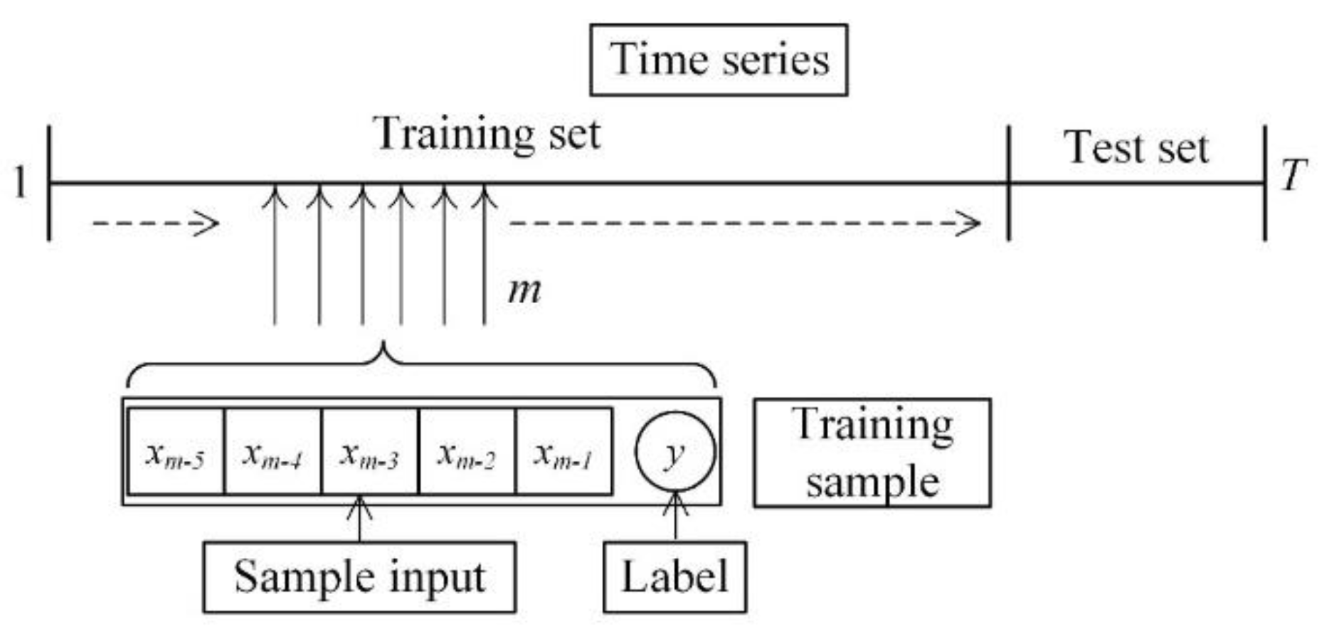
3.2.1. Model Inputs

In the experiments, GNSS measured displacements acquired monthly (from July 2003 to March 2013 for Baishuihe landslide, from September 2007 to May 2015 for Shuping landslide), the associated daily reservoir water level and precipitation are used, all of which are normalized to the interval from 0 to 1 using the max–min normalization. These datasets are further divided into a training dataset and a test dataset. The training dataset (from July 2003 to August 2011 for Baishuihe landslide, from September 2007 to March 2014 for Shuping landslide) of the input layer are taken as inputs in the training process, and the remaining dataset is used to evaluate the performance of our proposed method.
For the input layer, the training dataset of single GNSS displacement time series can be denoted as Dm = {d1, d2, …, dm}, m represents the length of the time series. GNSS observations from July 2003 to August 2011 for the Baishuihe landslide and from September 2007 to March 2014 for the Shuping landslide are taken separately as training datasets in the training process. The remaining GNSS observations are used to evaluate the performance of our proposed method.
The way of sample division from each training dataset is shown in Figure 9. A sliding window with window length equals l and step size equal n is used. Thus, the length of each obtained sample is l (2 ≤ l < m), represented by Dtrain = {dml, dml+1, …, dm1} with the last y (1 ≤ y < l) serving as label sample and the other values (l − y) used as the sample input.
In this paper, the sliding window size is set to 6 by taking account of the typicality and quantity of the training samples, which stands for the half-cycle of the external factors to facilitate the recurrent layer to capture the temporal dynamics. The first five are input samples, the last 1 marked as the label. As suggested by [32], the model error increase as the value of y increases; thus, we set it to 1. Therefore, the dimension of the training sample is 93 and 74, separately. The test datasets are treated in the same way.
For the Baishuihe landslide, a 7 × 7 weighted adjacency matrix Aw is first construed using the Gaussian similarity function based on the spatial proximity of the deployed GNSS monitoring stations (Section 2.2.1). Then a feature matrix X with a size of 7 × 117 is constructed to represent the temporal displacement of each station. The number of rows equals the number of stations; the number of columns equals the measured displacement time series. Thus, in the same way, the dimension of Aw and X for the Shuping landslide is 6 × 6 and 6 × 93, respectively.
As illustrated in Section 2.1, for both landslides, the fluctuation of the reservoir water level and varying precipitation are two main external factors influencing landslides behaviours. We introduce an attribute-augmented unit that integrates features of the displacements, the seasonal rainfall, and the water level fluctuation to represent the effect of external influencing factors on landslide deformation. The augmented matrix with weighted adjacency matrices is incorporated into the forecast model to enhance the extraction of realistic spatial–temporal dependency, and the derived results will be used as the model inputs.

3.2.2. Model Parameters and Settings

Our proposed model has four hyper-parameters: the learning rate, the number of training iteration epochs, the number of hidden units, and the batch size. In the experiment, we empirically set the learning rate to 0.001 and the batch size to 32 [33]. However, the numbers of training iteration epochs and hidden units are two crucial parameters that may affect the prediction precision and, therefore, should be determined by designed comparison experiments. The ReLU is employed as the activation for each convolutional layer and the Adam optimizer for minimizing the loss function (Equation (13)).
l o s s = t = 1 n ( Y t Y ^ t ) 2 / n
where n is the time series length, Y t represents the actual measurement, Y ^ t denotes the predicted value.
Comparison experiments for selecting the optimal hyper-parameters are performed by setting the number of hidden units to 64 first to analyze the changes of the prediction precision with a varying number of training epochs designed to be {100, 250, 500, 1000, 1500, 2000}. Figure 10 shows the variation of metrics with different training epochs. The horizontal axis represents the number of training epochs, and the vertical axis represents the variation of the metrics; it can be seen that when the training epochs equals 1000, the metrics obtain a minimum value. Thus, the model reaches its optimal performance. Accordingly, in the following comparison experiments, we set the training epochs value to 1000 to analyze the changes of the prediction precision with varying numbers of hidden units; these numbers are designed to be {8, 16, 32, 64, 100, 128}. Figure 11 gives the variation of metrics with different hidden units. The horizontal axis represents the number of hidden units, and the vertical axis represents the variation of the metrics. It can be seen that when the hidden units equal 64, the metrics obtain a minimum value. Thus, the model reaches its optimal performance. Consequently, in the following experiment, the number of training epochs and hidden units is set to be 1000 and 64, respectively.

3.3. Predicted Results and Analysis

3.3.1. Predicted Results Using the GC-GRU-N

To prove the effectiveness of the proposed model, we use four classical prediction models, which are MLR, ARIMA, SVR, and LSTM, to compare with the GC-GRU-N model for the two study sites. This section also conducts comparative analysis using the temporal graph convolutional network (T-GCN) without attribute augmentation to verify the model enhancement using the attribute-augmented graph convolution (GC) operations. We evaluate the effect of the GC-GRU-N model from two aspects: prediction performance and modelling time.
As the above-mentioned classical prediction models can only realize single time-series prediction, the model predictions only reflect the displacement behaviour of a single monitoring station. Thus, for a GNSS network with m stations, classic models need to calculate m times separately to obtain the displacement forecasts of all stations. The GC-GRU-N utilizes a feature matrix Xm×n (Section 3.2.1) to represent the displacement over time of each station, predicting the displacement of the entire monitoring system.
The predicted results of the Baishuihe landslide and the Shuping landslide by the proposed model are shown in Figure 12 and Figure 13, respectively. The predictions of each monitoring station are consistent well with the actual observations as a whole. According to Figure 6 and Figure 7, measurements of several monitoring stations show mutational transition appeared in September each year; a more significant prediction error arises at this abrupt state with a maximum of 16.66 mm and 30.35 mm, respectively. The maximum error does not exceed 10 mm for the rest of the year. It could be due to fewer samples being available for the mutation state than for the other states because a monthly prediction time scale is used due to data acquisition limitations. Generally speaking, as the number of samples for mutation state increases, e.g., with daily-scale displacement, the model’s errors gradually decrease. In addition, since the GCN captures spatial features by constantly moving a smooth filter in the Fourier domain, it might also lead to the peaks being smoother.

3.3.2. Comparative Experiments

The performance of the forecast models is shown in Table 3. Our proposed model has outperformed the other five models in terms of three evaluation indicators in two study areas (Table 3). The errors of models such as MLR, ARIMA, and SVR are relatively large, resulting in poor prediction performance. However, the LSTM as a neural network model is better than traditional machine learning models (SVR) and time series models (MLR and ARIMA). Compared with the LSTM model, the GC-GRU-N and the T-GCN model can better describe the displacement trend because the model structure captures the spatial feature of the monitoring network. Consequently, the prediction accuracy of the GC-GRU-N is effectively enhanced. For the Baishuihe landslide, the three metrics of GC-GRU-N are 3.682 mm of MAE, 0.477 of MASE, and 4.429 mm of RMSE, respectively.
In the following discussion, we use the RMSE as the primary metric to represent the model’s performance. The RMSE of the GC-GRU-N model and T-GCN model are reduced by approximately 64% and 50% compared with the MLR model. In comparison, the RMSE of the T-GC-GRU-N model and T-GCN model are around 56% and 38% lower than that of the ARIMA model. Compared with the SVR model, the RMSEs of the GC-GRU-N model and T-GCN model are reduced by 58% and 41%, respectively. In contrast, the RMSEs of the T-GC-GRU-N model and T-GCN model are decreased by 47% and 41% compared with the LSTM. Compared with the GC-GRU-N model, the T-GCN model is less effective because the T-GCN considers the spatial features and ignores the impact of the external factors on landslide displacement.
In terms of computation time, T-GCN is the most efficient model amongst all tested models, only requiring 19.93 s (Table 3). The proposed GC-GRU-N achieves competitive training efficiency ranking top two, taking 44.88 s, followed by the LSTM model costing 229.936 s. The GC-GRU-N is slower than T-GCN because the method needs to develop a unit to represent the effects of the triggering factors during convolution operation. The SVR takes 349.971 s, slightly higher than LSTM. In contrast, the modelling time of the MLR model and the ARIMA model is much longer than other methods presented in this paper, requiring 986.435 s and 0.534 h, respectively. In summary, the GC-GRU-N is significantly efficient considering its high accuracy among other advanced models.
Results of the ZG93 station installed on the Baishuihe landslide and the ZG85 station deployed on the Shuping landslide are depicted in Figure 14. The predictions of the proposed model are consistently well with the actual deformation trend and superior to other methods as a whole. Despite sometimes overreacting to rapid decreases and producing underestimated results at abrupt increases, our model outperforms all other time series forecast models at both landslides. This result indicates that the graph convolution with spatial correlation consideration scheme can efficiently capture the dynamics in the landslide monitoring.
Specifically, MLR and ARIMA as statistics methods can also depict the variation trend of landslide displacement, but with more significant overestimated or underestimated errors. The LSTM model is more efficient and shows more promising results than the SVR model in the machine-learning-based models, especially in predicting displacement around transition states. However, sudden rapid changes in the evolution may increase the model’s errors. This could be due to fewer samples being available for the mutation state.
The T-GCN and the GC-GRU-N models capturing spatial and temporal features have achieved more promising time-series forecasts. The T-GCN model gives a lower prediction accuracy. This is because the T-GCN model only considers the spatial features, and ignores the external factors impacting landslide displacement. In summary, the GC-GRU-N as a spatial and temporal mode is significantly efficient with high accuracy amongst other models in landslide displacement forecasting.

3.3.3. Ablation Experiment and Analysis

Ablation is utilized to demonstrate the importance of attribute enhancement to improve model performance. It refers to an attribute-augmented unit in the forecast model. We design the ablation experiment as the following: only consider the rainfall factor or the reservoir water effect, and both factors together (Figure 15). Table 4 shows the results for the Baishuihe landslide, with the T-GCN representing a model without an attribute-augmented unit. According to Table 4, the performance gains of using an attribute-augmented unit is apparent.
We also use the RMSE as the primary metric to represent the model’s performance. As the experiment considers the rainfall factor alone, the reservoir water level factor alone, and both factors together, the RMSE values of the proposed model are 4.442 mm, 4.434 mm, and 4.429 mm, respectively, all of which are lower than that of the T-GCN (6.183 mm). Specifically, the ablation experiment demonstrates the effectiveness of assembling the external inducing factors in graph convolutional network, and the best performance in all indicators is achieved when both factors are considered simultaneously. As shown in Figure 15, the predictions of considering both trigging factors are consistent well with the actual deformation trend, which is superior to the other two scenarios and is still valid around transition states, including rapid decrease and abrupt increase conditions.

4. Discussion

4.1. Advantage of the Proposed Method

Unlike the time-series forecast models that only explore temporal features and focus on a single point, this paper presents a new deep learning architecture that considers the spatial and temporal correlation for landslide displacement prediction. More specifically, the spatial correlation of the entire monitoring system and the temporal dependency of the monitoring time series are explored to establish the forecast model predicting the displacement of the monitoring network instead of a specific station. Considering the displacement prediction of a landslide relies not only on historical GNSS measurements and the spatial correlations of the monitoring network but also on various external incentive factors. An attribute-augmented unit is designed to integrate weighted adjacency matrix, displacements, and triggering factors to enhance the capture of spatial–temporal dependency serving as the model inputs.
To the best of the authors’ knowledge, there is currently no related work focusing on addressing the prediction of rainfall reservoir-induced landslide displacement from a holistic perspective combining the external incentive factors. This paper presents a new deep learning GC-GCN-N model based on the GCN and GRU models, which effectively utilizes the spatial and temporal features contained in the model input data. The results show that the proposed model outperforms comparative models in both landslides over our study site in China’s Three Gorge Reservoir (TGR).

4.2. Shortcoming and Outlook of the Proposed Method

As shown in Figure 6 and Figure 7, several GNSS-monitored displacements show mutational transitions in September. Accordingly, significant prediction error often appears at this abrupt state (Figure 12, Figure 13 and Figure 14), which is true to other forecast models. Considering the monthly data-acquisition limitation, this could be due to fewer samples available for the mutation state than for the other states. Thus, the model’s errors probably gradually decrease as the number of samples for the mutation state increases. In addition, the GCN captures spatial features by constantly moving a smooth filter in the Fourier domain, which might also lead to the peaks being smoother.
Limited datasets in geohazard domains might be a prevalent phenomenon. Results of the Shuping landslide and the Baishuihe landslide also show that the number of motoring stations in a GNSS network also affects the prediction result. As monitoring equipment and data transmission technology advance, daily, hourly, and even minute-scale displacements could be collected and predicted in real time. Additionally, several other solutions have emerged in different domains for handling dataset limitations, including data augmentation [34], synthetic data [35], and transfer learning [36].
Data augmentation refers to increasing the number of data points without changing the label. For example, variable factors include random noise, and adequate time characteristics can be employed to enlarge the time-series data [34]. Although not real data, synthetic data contain the same patterns and statistical properties as actual data, generated by a deep-learning model called generative adversarial networks (GAN) [35]. Transfer learning uses knowledge from other relevant datasets or an existing model to construct new models that lack enough training data to provide an alternative solution [23,36].
In this study, periodic rainfall and reservoir water level fluctuations are the main factors triggering landslide kinematic evolution in the TGR area. Therefore, we consider only these two trigging factors. Subsequent studies might include more complicated datasets to establish a more comprehensive model. For example, factors affecting landslide motion can consist of other essential characteristics of landslides, such as strata lithology, slope aspect and angle, etc.

5. Conclusions

This research develops a new deep-learning approach for landslide displacement forecasting called GC-GCN-N, which combines the GCN and the GRU. The architecture inherits the merits from both GCN in extracting spatial dependencies and GRU in capturing temporal correlation features to tackle the spatiotemporal landslide displacement forecast. In the proposed model, (1) a weighted adjacency matrix is built to interpret the spatial correlations between all monitoring stations, (2) a feature matrix is assembled to handle the time-series measurements of all monitoring stations, (3) an attribute-augmented unit is designed to represent the effects of the triggering factors and integrate the matrix mentioned above into a single graph convolutional network, and (4) a novel neural network-based approach is developed to enable to process the above graph-structured data. Experiments have been carried out on two landslides in Three George Reservoir, China. Compared with the MLR model, the ARIMA model, the SVR model, the LSTM model, and the T-GCN model, the GC-GCN-N model outperforms other forecasting models at both landslide sites. In summary, the GC-GCN-N model successfully captures the spatial and temporal features from the landslide monitoring dataset, showing great potential for other spatiotemporal forecast tasks.

Author Contributions

Conceptualization, Q.X. and Y.J.; methodology and validation, Y.J. and H.L. (Huiyuan Luo); formal analysis and investigation, L.L. resources, Q.X. and H.L.(Huajin Li); writing—original draft preparation, Y.J.; writing—review and editing, Y.J. and Z.L.; visualization, H.L. (Huiyuan Luo); funding acquisition, Q.X., L.H. and Y.J. All authors have read and agreed to the published version of the manuscript.

Funding

This research is financially supported by the National Key Research and Development Program of China (2018YFC1505101, 2021YFC3000401). The Key Research and Development Program of Sichuan Province (2020YFS0353) and the Open Fund of State Key Laboratory of Geohazard Prevention and Geoenviroment Protection (SKLGP2017K016).

Institutional Review Board Statement

Not applicable.

Informed Consent Statement

Not applicable.

Data Availability Statement

The raw data used in this study can be downloaded for scientific research after approval at http://www.crensed.ac.cn/, accessed on 14 February 2022.

Acknowledgments

The authors would like to thank the National Service Center for Specialty Environmental Observation Stations for providing the in situ monitoring data set.

Conflicts of Interest

The authors declare no conflict of interest.

References

  1. Runqiu, H. Some Catastrophic Landslides since the Twentieth Century in the Southwest of China. Landslides 2009, 6, 69–81. [Google Scholar] [CrossRef]
  2. Hu, X.; Bürgmann, R.; Schulz, W.H.; Fielding, E.J. Fielding. Four-Dimensional Surface Motions of the Slumgullion Landslide and Quantification of Hydrometeorological Forcing. Nat. Commun. 2020, 11, 2792–2801. [Google Scholar] [CrossRef] [PubMed]
  3. Fan, X.; Scaringi, G.; Korup, O.; West, A.J.; van Westen, C.J.; Tanyas, H.; Hovius, N.; Hales, T.C.; Jibson, R.W.; Allstadt, K.E.; et al. Earthquake-Induced Chains of Geologic Hazards: Patterns, Mechanisms, and Impacts. Rev. Geophys. 2019, 57, 421–503. [Google Scholar] [CrossRef] [Green Version]
  4. Jiang, Y.; Xu, Q.; Lu, Z.; Luo, H.; Liao, L.; Dong, X. Modelling and Predicting Landslide Displacements and Uncertainties by Multiple Machine-Learning Algorithms: Application to Baishuihe Landslide in Three Gorges Reservoir, China. Geomat. Nat. Hazards Risk 2021, 12, 741–762. [Google Scholar] [CrossRef]
  5. LeCun, Y.; Bengio, Y.; Hinton, G. Deep Learning. Nature 2015, 521, 436–444. [Google Scholar] [CrossRef] [PubMed]
  6. Ma, Z.; Mei, G. Deep Learning for Geological Hazards Analysis: Data, Models, Applications, and Opportunities. Earth Sci. Rev. 2021, 223, 103858. [Google Scholar] [CrossRef]
  7. Krkač, M.; Bernat Gazibara, S.; Arbanas, Ž.; Sečanj, M.; Mihalić Arbanas, S. A Comparative Study of Random Forests and Multiple Linear Regression in the Prediction of Landslide Velocity. Landslides 2020, 17, 2515–2531. [Google Scholar] [CrossRef]
  8. Zhang, G.P. Time Series Forecasting Using a Hybrid ARIMA and Neural Network Model. Neurocomputing 2003, 50, 159–175. [Google Scholar] [CrossRef]
  9. Zhang, Y.; Tang, J.; He, Z.; Tan, J.; Li, C. A Novel Displacement Prediction Method Using Gated Recurrent Unit Model with Time Series Analysis in the Erdaohe Landslide. Nat. Hazards 2021, 105, 783–813. [Google Scholar] [CrossRef]
  10. Xu, S.; Niu, R. Displacement Prediction of Baijiabao Landslide Based on Empirical Mode Decomposition and Long Short-Term Memory Neural Network in Three Gorges Area, China. Comput. Geosci. 2018, 111, 87–96. [Google Scholar] [CrossRef]
  11. Li, H.; Xu, Q.; He, Y.; Fan, X.; Li, S. Modeling and Predicting Reservoir Landslide Displacement with Deep Belief Network and EWMA Control Charts: A Case Study in Three Gorges Reservoir. Landslides 2020, 17, 693–707. [Google Scholar] [CrossRef]
  12. Han, H.; Shi, B.; Zhang, L. Prediction of Landslide Sharp Increase Displacement by SVM with Considering Hysteresis of Groundwater Change. Eng. Geol. 2021, 280, 105876. [Google Scholar] [CrossRef]
  13. Lv, M.; Hong, Z.; Chen, L.; Chen, T.; Zhu, T.; Ji, S. Temporal Multi-Graph Convolutional Network for Traffic Flow Prediction. IEEE Trans. Intell. Transp. Syst. 2021, 22, 3337–3348. [Google Scholar] [CrossRef]
  14. Huang, Y.; Han, X.; Zhao, L. Recurrent Neural Networks for Complicated Seismic Dynamic Response Prediction of a Slope System. Eng. Geol. 2021, 289, 106198. [Google Scholar] [CrossRef]
  15. Chen, P.; Fu, X.; Wang, X. A Graph Convolutional Stacked Bidirectional Unidirectional-LSTM Neural Network for Metro Ridership Prediction. IEEE Trans. Intell. Transp. Syst. 2021, 1–13. [Google Scholar] [CrossRef]
  16. Navarin, N.; Van Tran, D.; Sperduti, A. Universal Readout for Graph Convolutional Neural Networks. In Proceedings of the 2019 International Joint Conference on Neural Networks (IJCNN), Budapest, Hungary, 14–19 July 2019; IEEE: Piscataway, NJ, USA, 2019; pp. 1–7. [Google Scholar]
  17. Panahi, M.; Sadhasivam, N.; Pourghasemi, H.R.; Rezaie, F.; Lee, S. Spatial Prediction of Groundwater Potential Mapping Based on Convolutional Neural Network (CNN) and Support Vector Regression (SVR). J. Hydrol. 2020, 588, 125033. [Google Scholar] [CrossRef]
  18. Jepsen, T.S.; Jensen, C.S.; Nielsen, T.D. Relational Fusion Networks: Graph Convolutional Networks for Road Networks. IEEE Trans. Intell. Transp. Syst. 2020, 23, 418–429. [Google Scholar] [CrossRef]
  19. Jiang, Y.; Liao, M.; Zhou, Z.; Shi, X.; Zhang, L.; Balz, T. Landslide Deformation Analysis by Coupling Deformation Time Series from SAR Data with Hydrological Factors through Data Assimilation. Remote Sens. 2016, 8, 179. [Google Scholar] [CrossRef] [Green Version]
  20. Jiang, C.; Fan, W.; Yu, N.; Liu, E. Spatial Modeling of Gully Head Erosion on the Loess Plateau Using a Certainty Factor and Random Forest Model. Sci. Total Environ. 2021, 783, 147040. [Google Scholar] [CrossRef]
  21. Deng, L.; Smith, A.; Dixon, N.; Yuan, H. Machine Learning Prediction of Landslide Deformation Behaviour Using Acoustic Emission and Rainfall Measurements. Eng. Geol. 2021, 106315. [Google Scholar] [CrossRef]
  22. Hu, X.; Wu, S.; Zhang, G.; Zheng, W.; Liu, C.; He, C.; Liu, Z.; Guo, X.; Zhang, H. Landslide Displacement Prediction Using Kinematics-Based Random Forests Method: A Case Study in Jinping Reservoir Area, China. Eng. Geol. 2021, 283, 105975. [Google Scholar] [CrossRef]
  23. Long, J.; Li, C.; Liu, Y.; Feng, P.; Zuo, Q. A Multi-Feature Fusion Transfer Learning Method for Displacement Prediction of Rainfall Reservoir-Induced Landslide with Step-like Deformation Characteristics. Eng. Geol. 2022, 297, 106494. [Google Scholar] [CrossRef]
  24. Shin, Y.; Yoon, Y. Incorporating Dynamicity of Transportation Network With Multi-Weight Traffic Graph Convolutional Network for Traffic Forecasting. IEEE Trans. Intell. Transp. Syst. 2020, 1–11. [Google Scholar] [CrossRef]
  25. Ma, Z.; Mei, G.; Prezioso, E.; Zhang, Z.; Xu, N. A Deep Learning Approach Using Graph Convolutional Networks for Slope Deformation Prediction Based on Time-Series Displacement Data. Neural Comput. Appl. 2021, 33, 14441–14457. [Google Scholar] [CrossRef]
  26. Yao, X.; Gao, Y.; Zhu, D.; Manley, E.; Wang, J.; Liu, Y. Spatial Origin-Destination Flow Imputation Using Graph Convolutional Networks. IEEE Trans. Intell. Transp. Syst. 2020, 22, 7474–7484. [Google Scholar] [CrossRef]
  27. Bengio, Y.; Simard, P.; Frasconi, P. Learning Long-Term Dependencies with Gradient Descent Is Difficult. IEEE Trans. Neural Netw. 1994, 5, 157–166. [Google Scholar] [CrossRef]
  28. Hochreiter, S.; Schmidhuber, J. Long Short-Term Memory. Neural Comput. 1997, 9, 1735–1780. [Google Scholar] [CrossRef]
  29. Cho, K.; van Merrienboer, B.; Bahdanau, D.; Bengio, Y. On the Properties of Neural Machine Translation: Encoder-Decoder Approaches. arXiv 2014, arXiv:1409.1259. [Google Scholar]
  30. Man, J.; Dong, H.; Yang, X.; Meng, Z.; Jia, L.; Qin, Y.; Xin, G. GCG: Graph Convolutional Network and Gated Recurrent Unit Method for High-Speed Train Axle Temperature Forecasting. Mech. Syst. Signal Process. 2022, 163, 108102. [Google Scholar] [CrossRef]
  31. Hyndman, R.J.; Koehler, A.B. Another Look at Measures of Forecast Accuracy. Int. J. Forecast. 2006, 22, 679–688. [Google Scholar] [CrossRef] [Green Version]
  32. Qinghao, L.I.U.; Yonghong, Z.; Min, D.; Hongan, W.U.; Yonghui, K.; Jujie, W.E.I. Time Series Prediction Method of Large-Scale Surface Subsidence Based on Deep Learning. Acta Geod. Cartogr. Sin. 2021, 50, 396. [Google Scholar] [CrossRef]
  33. Zhao, L.; Song, Y.; Zhang, C.; Liu, Y.; Wang, P.; Lin, T.; Deng, M.; Li, H. T-GCN: A Temporal Graph Convolutional Network for Traffic Prediction. IEEE Trans. Intell. Transp. Syst. 2020, 21, 3848–3858. [Google Scholar] [CrossRef] [Green Version]
  34. Rashid, K.M.; Louis, J. Times-Series Data Augmentation and Deep Learning for Construction Equipment Activity Recognition. Adv. Eng. Inform. 2019, 42, 100944. [Google Scholar] [CrossRef]
  35. Creswell, A.; White, T.; Dumoulin, V.; Arulkumaran, K.; Sengupta, B.; Bharath, A.A. Generative Adversarial Networks: An Overview. IEEE Signal Process. Mag. 2018, 35, 53–65. [Google Scholar] [CrossRef] [Green Version]
  36. Li, N.; Hao, H.; Gu, Q.; Wang, D.; Hu, X. A Transfer Learning Method for Automatic Identification of Sandstone Microscopic Images. Comput. Geosci. 2017, 103, 111–121. [Google Scholar] [CrossRef]
Figure 1. The workflow of the proposed model.
Remotesensing 14 01016 g001
Figure 2. Location of the study area and the overall view of the two landslides.
Remotesensing 14 01016 g002
Figure 3. Monitoring data in time series of the Baishuihe landslide.
Remotesensing 14 01016 g003
Figure 4. Monitoring data in time series of the Shuping landslide.
Remotesensing 14 01016 g004
Figure 5. The diagram of a weighted graph and adjacency matrix.
Remotesensing 14 01016 g005
Figure 6. The architectures of two deep-learning models: (a) the graph convolution networks; (b) the gated recurrent units.
Remotesensing 14 01016 g006
Figure 7. The overall process of spatiotemporal prediction.
Remotesensing 14 01016 g007
Figure 8. (ad) Deformation over time of adjacent monitoring points of different pairs.
Remotesensing 14 01016 g008
Figure 9. The sample division of a single time series.
Remotesensing 14 01016 g009
Figure 10. The variation of metrics with different training epochs.
Remotesensing 14 01016 g010
Figure 11. The variation of metrics with different hidden units.
Remotesensing 14 01016 g011
Figure 12. Comparison diagram of the overall prediction of landslide displacement; the vertical purple line represents the absolute error.
Remotesensing 14 01016 g012
Figure 13. Comparison diagram of the overall prediction of landslide displacement; the vertical purple line represents the absolute error.
Remotesensing 14 01016 g013
Figure 14. Comparison results of the proposed model and five other models. Results of ZG93 installed on the Baishuihe landslide are shown in figure (a,b), and that of ZG85 deployed on the Shuping landslide are shown in figure (c,d).
Remotesensing 14 01016 g014
Figure 15. Comparison results of the ablation experiments considering only the rainfall factor or the reservoir water effect, and both factors together. The solid black line represents the original value.
Remotesensing 14 01016 g015
Table 1. Grey relation analysis results of the Shuping landslide.
PointZG85ZG86ZG87ZG88SP-2SP-6
ZG8510.780.870.820.800.84
ZG860.7810.880.750.860.85
ZG870.870.8810.880.870.88
ZG880.820.750.8810.830.82
SP-20.800.860.870.8310.75
SP-60.840.850.880.820.751
Table 2. Grey relation analysis results of the Baishuihe landslide.
PointZG91ZG92ZG93ZG94ZG118ZG119ZG120
ZG911.000.690.510.760.520.790.77
ZG920.691.000.540.700.570.650.65
ZG930.510.541.000.590.740.540.59
ZG940.760.700.591.000.590.720.71
ZG1180.520.570.740.591.000.550.54
ZG1190.790.650.540.720.551.000.68
ZG1200.770.650.590.710.540.681.00
Table 3. The performance of different forecast models.
ModelEvaluation IndexAverage Time
BaishuiheShuping
MAE/mmMASERMSE/mmMAE/mmMASERMSE/mm
The proposed3.6820.4774.4296.1230.3538.32144.88 s
T-GCN4.7070.616.1837.0710.4019.79619.93 s
MLR7.5140.97412.31913.5480.78217.566986.435 s
ARIMA6.7180.8710.04110.9530.63213.9170.534 h
SVR6.7650.87710.51213.9360.80416.734349.971 s
LSTM5.9810.7278.4018.8250.50912.788229.936 s
Table 4. Ablation Experiments with different settings.
Evaluation IndexT-GCNThe Proposed Model (the Baishuihe Landslide)
RainfallR.w.lBoth Factors
MAE/mm4.7073.7243.7043.682
MASE0.6100.4910.4890.477
RMSE/mm6.1834.4424.4344.429
Note: R.w.l is the reservoir water level.
Publisher’s Note: MDPI stays neutral with regard to jurisdictional claims in published maps and institutional affiliations.

