
Sentinel-2 Data and Unmanned Aerial System Products to Support Crop and Bare Soil Monitoring: Methodology Based on a Statistical Comparison between Remote Sensing Data with Identical Spectral Bands

 , ,
, ,  and
and
Abstract
:1. Introduction
2. Study Area and Materials
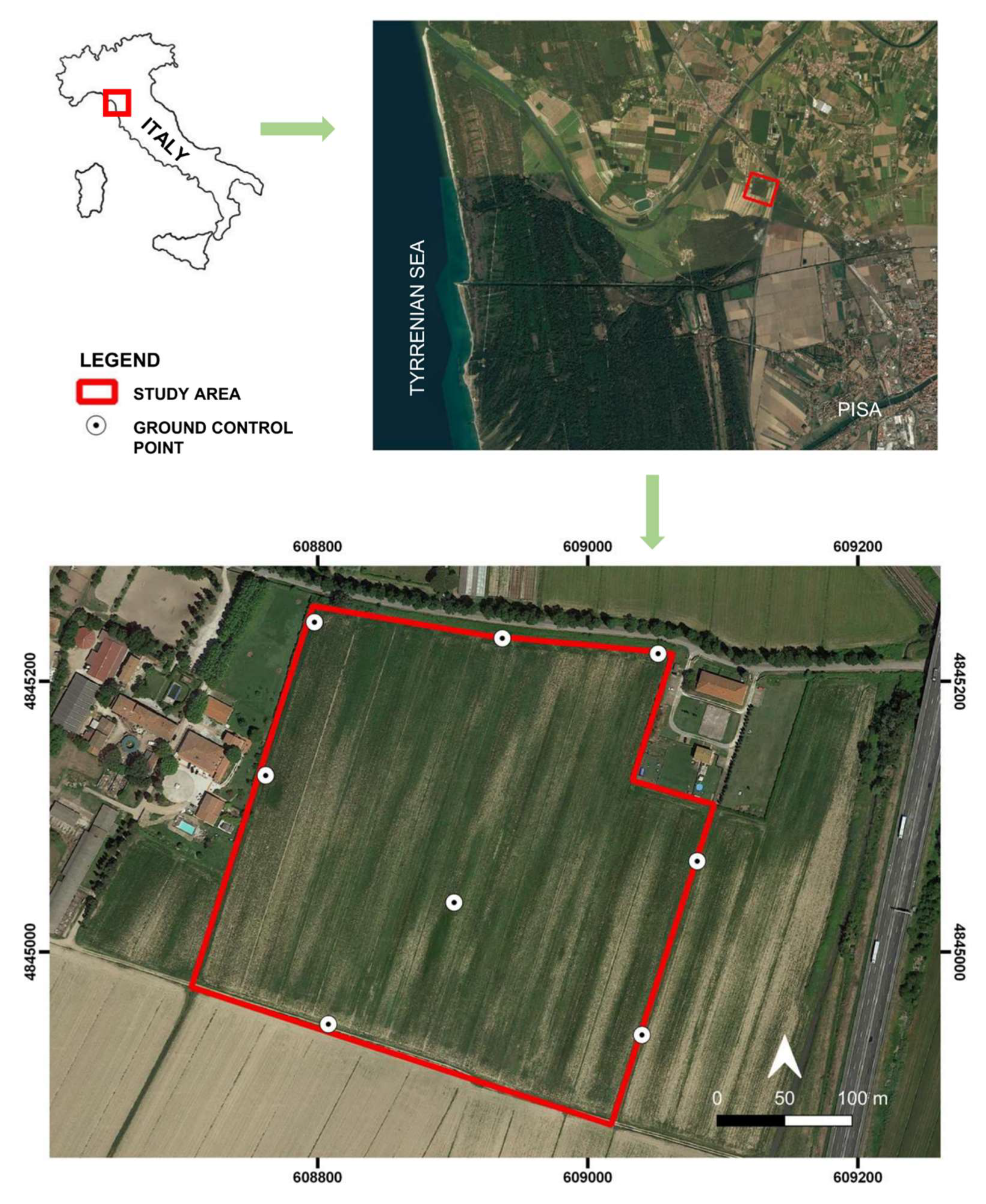
2.1. Study Area
2.2. Data
3. Methods
3.1. Georeferencing
3.2. Data Accuracy
3.3. Test Area Choice and Vegetation Index Applications
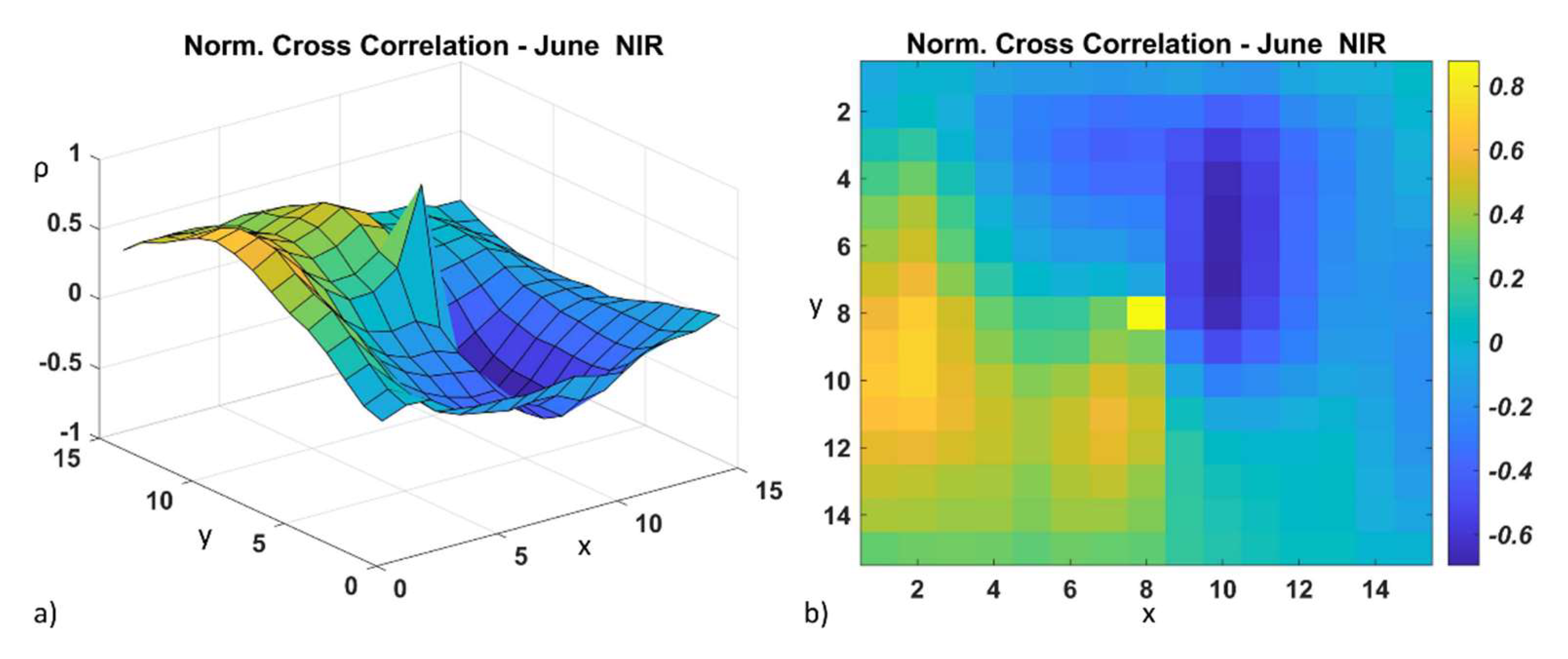
3.4. Statistical Test
3.5. Linear Regression
4. Results
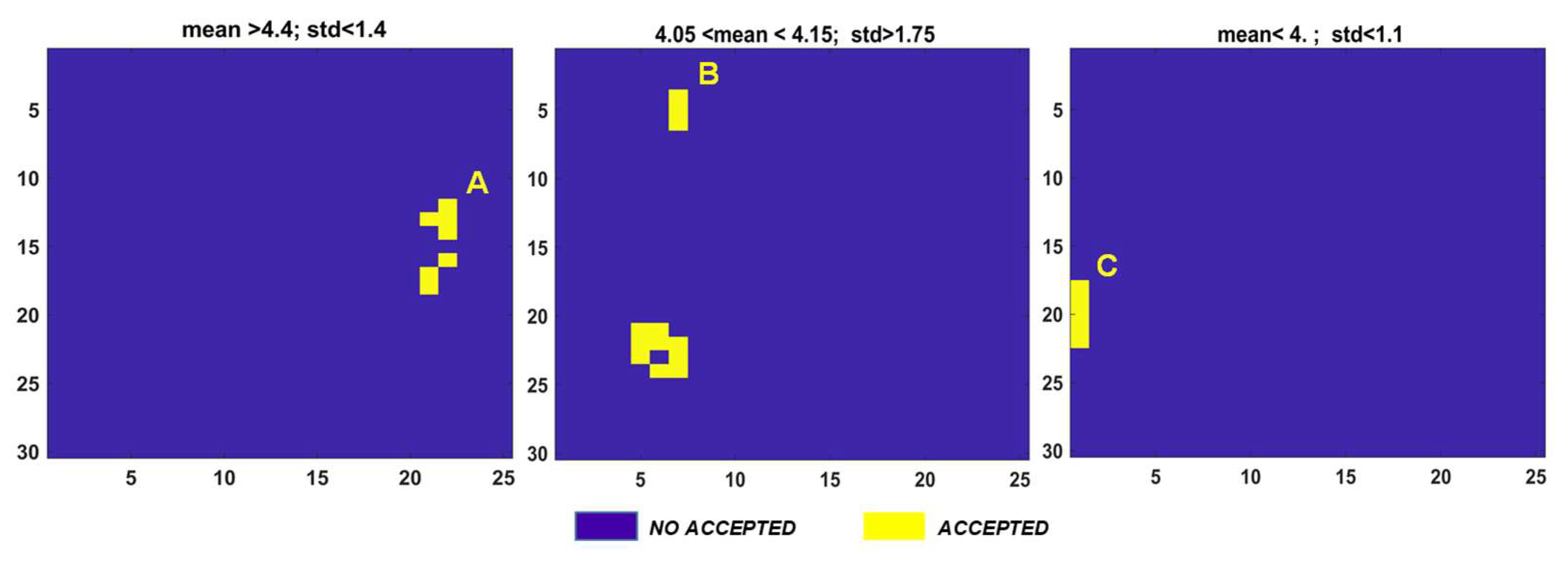
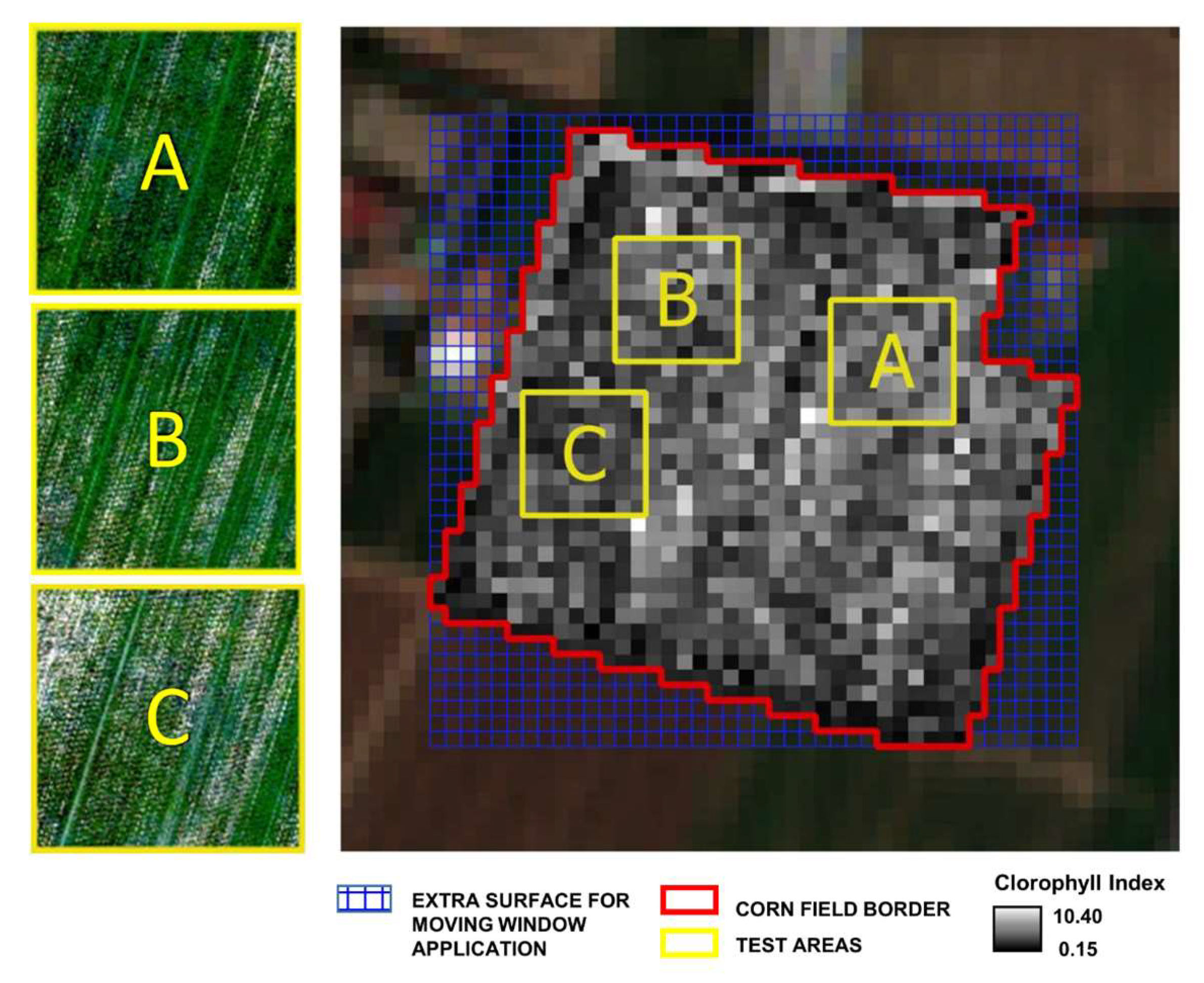
4.1. Test Areas
4.2. Vegetation Index and Statistical Test Results
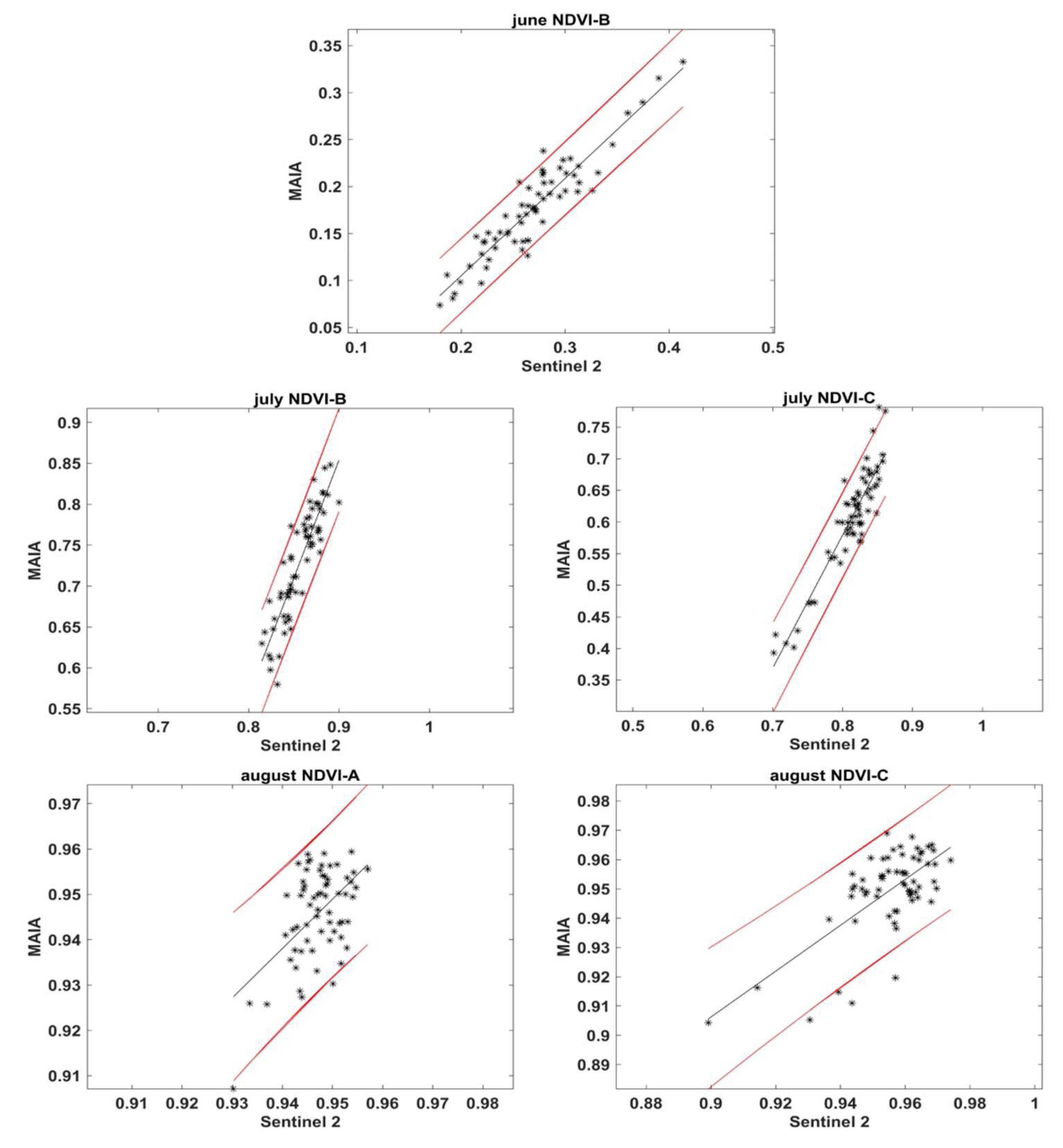
4.3. Linear Regression: MS2_10 NDVI vs. S2 NDVI
5. Discussion
- −
- it allows the identification of different behaviors of the relationship between bare soil and crop, and their mixture;
- −
- it allows the application of the most suitable and diversified analysis strategy within each subarea until the completion of the entire plot. The mobile window used was also essential for characterizing the entire plot and,
- −
- the transfer of the method to different types of crop systems characterized by areas with different percentages of vegetation cover.
6. Conclusions
- −
- for June, for NIR data in area A, B and C;
- −
- for August, for NDVI values in test areas A and C, Red data in test area A and NIR data in all test areas.
- −
- in August, MS2 data can become ground truths suitable for calibrating information extracted from satellite data;
- −
- in June, MS2 data can complement and extend S2 measurements.
Author Contributions
Funding
Institutional Review Board Statement
Informed Consent Statement
Data Availability Statement
Acknowledgments
Conflicts of Interest
References
- Lipper, L.; Thornton, P.; Campbell, B.M.; Baedeker, T.; Braimoh, A.K.; Bwalya, M.; Caron, P.; Cattaneo, A.; Garrity, D.P.; Henry, K.; et al. Climate-smart agriculture for food security. Nat. Clim. Chang. 2014, 4, 1068–1072. [Google Scholar] [CrossRef]
- Way, D.A.; Long, S.P. Climate-smart agriculture and forestry: Maintaining plant productivity in a changing world while minimizing production system effects on climate. Plant Cell Environ. 2015, 38, 1683–1685. [Google Scholar] [CrossRef] [PubMed]
- United Nations. Sustainable Development Goals: Goal 2 Zero Hunger. Available online: https://www.un.org/sustainabledevelopment/hunger/ (accessed on 21 September 2020).
- FAO. The Future of Food and Agriculture-Trends and Challenges; Food and Agriculture Organization of the United Nations: Rome, Italy, 2017; Volume 296, pp. 1–180. [Google Scholar]
- FAOSTAT. Food and Agriculture Organization Corporate Statistical Database (FAOSTAT) 29. 2018. Available online: http://www.fao.org/faostat/en/#home (accessed on 30 December 2020).
- IPCC. Climate change and land, the Intergovernmental Panel on Climate Change. In Special Report on Climate Change, Desertification, Land Degradation, Sustainable Land Management, Food Security, and Greenhouse Gas Fluxes in Terrestrial Ecosystems; IPCC: Geneva, Switzerland, 2019; Chapter 5; pp. 1–200. [Google Scholar]
- Schiavon, E.; Taramelli, A.; Tornato, A.; Pierangeli, F. Monitoring environmental and climate goals for European agriculture: User perspectives on the optimization of the Copernicus evolution offer. J. Environ. Manag. 2021, 296, 113121. [Google Scholar] [CrossRef] [PubMed]
- Weiss, M.; Jacob, F.; Duveiller, G. Remote sensing for agricultural applications: A meta-review. Remote Sens. Environ. 2020, 236, 111402. [Google Scholar] [CrossRef]
- Inoue, Y. Satellite- and drone-based remote sensing of crops and soils for smart farming–A review. Soil Sci. Plant Nutr. 2020, 66, 798–810. [Google Scholar] [CrossRef]
- European Commission. Commission Implementing Regulation (EU) 2018/746 of 18 May 2018 Amending Implementing Regulation (EU) No 809/2014 as Regards Modification of Single Applications and Payment Claims and Checks; C/2018/2976, OJ L 125, 22.5.2018; EC: Brussels, Belgium, 2018; pp. 1–7. [Google Scholar]
- Gupta, M.; Abdelsalam, M.; Khorsandroo, S.; Mittal, S. Security and privacy in smart farming: Challenges and opportunities. IEEE Access 2020, 8, 34564–34584. [Google Scholar] [CrossRef]
- Moysiadis, V.; Sarigiannidis, P.; Vitsas, V.; Khelifi, A. Smart Farming in Europe. Comput. Sci. Rev. 2021, 39, 100345. [Google Scholar] [CrossRef]
- Wolfert, S.; Ge, L.; Verdouw, C.; Bogaardt, M.-J. Big data in smart farming—A review. Agric. Syst. 2017, 153, 69–80. [Google Scholar] [CrossRef]
- Lytos, A.; Lagkas, T.; Sarigiannidis, P.; Zervakis, M.; Livanos, G. Towards smart farming: Systems, frameworks and exploitation of multiple sources. Comput. Networks 2020, 172, 107147. [Google Scholar] [CrossRef]
- Taramelli, A.; Tornato, A.; Magliozzi, M.L.; Mariani, S.; Valentini, E.; Zavagli, M.; Costantini, M.; Nieke, J.; Adams, J.; Rast, M. An interaction methodology to collect and assess user-driven requirements to define potential opportunities of future hyperspectral imaging sentinel mission. Remote Sens. 2020, 12, 1286. [Google Scholar] [CrossRef] [Green Version]
- Murugan, D.; Garg, A.; Singh, D. Development of an adaptive approach for precision agriculture monitoring with drone and satellite data. IEEE J. Sel. Top. Appl. Earth Obs. Remote Sens. 2017, 10, 5322–5328. [Google Scholar] [CrossRef]
- Pla, M.; Bota, G.; Duane, A.; Balagué, J.; Curcó, A.; Gutiérrez, R.; Brotons, L. Calibrating Sentinel-2 Imagery with Multispectral UAV Derived Information to Quantify Damages in Mediterranean Rice Crops Caused by Western Swamphen (Porphyrio porphyrio). Drones 2019, 3, 45. [Google Scholar] [CrossRef] [Green Version]
- Yeom, J.; Jung, J.; Chang, A.; Ashapure, A.; Maeda, M.; Maeda, A.; Landivar, J. Comparison of vegetation indices derived from UAV data for differentiation of tillage effects in agriculture. Remote Sens. 2019, 11, 1548. [Google Scholar] [CrossRef] [Green Version]
- Bauer, M.E.; Cipra, J.E. Identification of agricultural crops by computer processing of ERTS MSS data. In Proceedings of the Symposium on Significant Results Obtained from the Earth Resources Technology Satellite-1, New Carrollton, MD, USA, 5–9 March 1973; Volume 1, pp. 205–212. [Google Scholar]
- Jürgens, C. The modified normalized difference vegetation index (mNDVI) a new index to determine frost damages in agriculture based on Landsat TM data. Int. J. Remote Sens. 1997, 18, 3583–3594. [Google Scholar] [CrossRef]
- Lyle, G.; Lewis, M.; Ostendorf, B. Testing the temporal ability of landsat imagery and precision agriculture technology to provide high resolution historical estimates of wheat yield at the farm scale. Remote Sens. 2013, 5, 1549–1567. [Google Scholar] [CrossRef] [Green Version]
- Akanwa, A.O.; Okeke, F.I.; Nnodu, V.C.; Iortyom, E.T. Quarrying and its effect on vegetation cover for a sustainable development using high-resolution satellite image and GIS. Environ. Earth Sci. 2017, 76, 505. [Google Scholar] [CrossRef]
- Upadhyay, P.; Kumar, A.; Roy, P.S.; Ghosh, S.; Gilbert, I. Effect on specific crop mapping using WorldView-2 multispectral add-on bands: Soft classification approach. J. Appl. Remote Sens. 2012, 6, 063524. [Google Scholar] [CrossRef]
- Primicerio, J.; Di Gennaro, S.F.; Fiorillo, E.; Genesio, L.; Lugato, E.; Matese, A.; Vaccari, F.P. A flexible unmanned aerial vehicle for precision agriculture. Precis. Agric. 2012, 13, 517–523. [Google Scholar] [CrossRef]
- Maresma, Á.; Ariza, M.; Martínez, E.; Lloveras, J.; Martínez-Casasnovas, J.A. Analysis of Vegetation Indices to Determine Nitrogen Application and Yield Prediction in Maize (Zea mays L.) from a Standard UAV Service. Remote Sens. 2016, 8, 973. [Google Scholar] [CrossRef] [Green Version]
- Deng, L.; Mao, Z.; Li, X.; Hu, Z.; Duan, F.; Yan, Y. UAV-based multispectral remote sensing for precision agriculture: A comparison between different cameras. ISPRS J. Photogramm. Remote Sens. 2018, 146, 124–136. [Google Scholar] [CrossRef]
- Li, J.; Zhang, F.; Qian, X.; Zhu, Y.; Shen, G. Quantification of rice canopy nitrogen balance index with digital imagery from unmanned aerial vehicle. Remote Sens. Lett. 2015, 6, 183–189. [Google Scholar] [CrossRef]
- Barbedo, J.G.A. Detection of nutrition deficiencies in plants using proximal images and machine learning: A review. Comput. Electron. Agric. 2019, 162, 482–492. [Google Scholar] [CrossRef]
- Radoglou-Grammatikis, P.; Sarigiannidis, P.; Lagkas, T.; Moscholios, I. A compilation of UAV applications for precision agriculture. Comput. Netw. 2020, 172, 107148. [Google Scholar] [CrossRef]
- Thapa, S.; Millan, V.G.; Eklundh, L. Assessing Forest Phenology: A Multi-Scale Comparison of Near-Surface (UAV, Spectral Reflectance Sensor, PhenoCam) and Satellite (MODIS, Sentinel-2) Remote Sensing. Remote Sens. 2021, 13, 1597. [Google Scholar] [CrossRef]
- Benincasa, P.; Antognelli, S.; Brunetti, L.; Fabbri, C.A.; Natale, A.; Sartoretti, V.; Modeo, G.; Guiducci, M.; Tei, F.; Vizzari, M. Reliability of NDVI derived by high resolution satellite and UAV compared to in-field methods for the evaluation of early crop N status and grain yield in wheat. Exp. Agric. 2018, 54, 604–622. [Google Scholar] [CrossRef]
- Mancini, A.; Frontoni, E.; Zingaretti, P. Satellite and UAV data for Precision Agriculture Applications. In Proceedings of the 2019 International Conference on Unmanned Aircraft Systems (ICUAS), Atlanta, GA, USA, 11–14 June 2019; pp. 491–497. [Google Scholar]
- Pastonchi, L.; Di Gennaro, S.F.; Toscano, P.; Matese, A. Comparison between satellite and ground data with UAV-based information to analyse vineyard spatio-temporal variability. OENO One 2020, 54, 919–934. [Google Scholar] [CrossRef]
- Kavosi, Z.; Raoufat, M.H.; Dehghani, M.; Abdolabbas, J.; Kazemeini, S.A.; Nazemossadat, M.J.; Dehghaani, M.; Jafari, A.; Kazemeini, A.; Naazemossadat, M.J. Feasibility of satellite and drone images for monitoring soil residue cover. J. Saudi Soc. Agric. Sci. 2020, 19, 56–64. [Google Scholar] [CrossRef]
- Müllerová, J.; Brůna, J.; Bartaloš, T.; Dvořák, P.; Vitkova, M.; Pyšek, P. Timing is important: Unmanned aircraft vs. satellite imagery in plant invasion monitoring. Front. Plant Sci. 2017, 8, 887. [Google Scholar] [CrossRef] [Green Version]
- Rudd, J.D.; Roberson, G.T.; Classen, J.J. Application of satellite, unmanned aircraft system, and ground-based sensor data for precision agriculture: A review. In Proceedings of the 2017 Spokane, Washington, DC, USA, 16 July–19 July 2017; American Society of Agricultural and Biological Engineers: St. Joseph, MI, USA, 2017; p. 1. [Google Scholar]
- Nonni, F.; Malacarne, D.; Pappalardo, S.E.; Codato, D.; Meggio, F.; De Marchi, M. Sentinel-2 Data Analysis and Comparison with UAV Multispectral Images for Precision Viticulture. GI_Forum 2018, 1, 105–116. [Google Scholar] [CrossRef]
- Messina, G.; Peña, J.; Vizzari, M.; Modica, G. A Comparison of UAV and Satellites Multispectral Imagery in Monitoring Onion Crop. An Application in the ‘Cipolla Rossa di Tropea’ (Italy). Remote Sens. 2020, 12, 3424. [Google Scholar] [CrossRef]
- Sozzi, M.; Kayad, A.; Marinello, F.; Taylor, J.; Tisseyre, B. Comparing vineyard imagery acquired from Sentinel-2 and Un-manned Aerial Vehicle (UAV) platform. Oeno One 2020, 54, 189–197. [Google Scholar] [CrossRef] [Green Version]
- Riihimäki, H.; Luoto, M.; Heiskanen, J. Estimating fractional cover of tundra vegetation at multiple scales using unmanned aerial systems and optical satellite data. Remote Sens. Environ. 2019, 224, 119–132. [Google Scholar] [CrossRef]
- Alvarez-Vanhard, E.; Corpetti, T.; Houet, T. UAV & satellite synergies for optical remote sensing applications: A literature review. Sci. Remote Sens. 2021, 3, 100019. [Google Scholar] [CrossRef]
- Gitelson, A.A. Wide dynamic range vegetation index for remote quantification of biophysical characteristics of vegetation. J. Plant Physiol. 2004, 161, 165–173. [Google Scholar] [CrossRef] [PubMed] [Green Version]
- Bendig, J.; Yu, K.; Aasen, H.; Bolten, A.; Bennertz, S.; Broscheit, J.; Gnyp, M.L.; Bareth, G. Combining UAV-based plant height from crop surface models, visible, and near infrared vegetation indices for biomass monitoring in barley. Int. J. Appl. Earth Obs. Geoinf. 2015, 39, 79–87. [Google Scholar] [CrossRef]
- Gevaert, C.; Suomalainen, J.; Tang, J.; Kooistra, L. Generation of Spectral-Temporal Response Surfaces by Combining Multispectral Satellite and Hyperspectral UAV Imagery for Precision Agriculture Applications. IEEE J. Sel. Top. Appl. Earth Obs. Remote Sens. 2015, 8, 3140–3146. [Google Scholar] [CrossRef]
- Mazzia, V.; Comba, L.; Khaliq, A.; Chiaberge, M.; Gay, P. UAV and Machine learning based refinement of a satellite-driven vegetation index for precision agriculture. Sensors 2020, 20, 2530. [Google Scholar] [CrossRef] [PubMed]
- Dubbini, M.; Pezzuolo, A.; De Giglio, M.; Gattelli, M.; Curzio, L.; Covi, D.; Yezekyan, T.; Marinello, F. Last generation instrument for agriculture multispectral data collection. Agric. Eng. Int. CIGR J. 2017, 19, 87–93. [Google Scholar]
- Chauhan, S.; Darvishzadeh, R.; Lu, Y.; Stroppiana, D.; Boschetti, M.; Pepe, M.; Nelson, A. Wheat lodging assessment using multispectral UAV data. ISPRS-Int. Arch. Photogramm. Remote Sens. Spat. Inf. Sci. 2019, XLII-2/W13, 235–240. [Google Scholar] [CrossRef] [Green Version]
- Caturegli, L.; Gaetani, M.; Volterrani, M.; Magni, S.; Minelli, A.; Baldi, A.; Brandani, G.; Mancini, M.; Lenzi, A.; Orlandini, S.; et al. Normalized Difference Vegetation Index versus Dark Green Colour Index to estimate nitrogen status on bermudagrass hybrid and tall fescue. Int. J. Remote Sens. 2019, 41, 455–470. [Google Scholar] [CrossRef]
- Tucker, C.J. Red and photographic infrared linear combinations for monitoring vegetation. Remote Sens. Environ. 1979, 8, 127–150. [Google Scholar] [CrossRef] [Green Version]
- Huete, A.R. A soil-adjusted vegetation index (SAVI). Remote Sens. Environ. 1988, 25, 295–309. [Google Scholar] [CrossRef]
- Fern, R.R.; Foxley, E.A.; Bruno, A.; Morrison, M.L. Suitability of NDVI and OSAVI as estimators of green biomass and coverage in a semi-arid rangeland. Ecol. Indic. 2018, 94, 16–21. [Google Scholar] [CrossRef]
- Insua, J.R.; Utsumi, S.A.; Basso, B. Estimation of spatial and temporal variability of pasture growth and digestibility in grazing rotations coupling unmanned aerial vehicle (UAV) with crop simulation models. PLoS ONE 2019, 14, e0212773. [Google Scholar] [CrossRef] [Green Version]
- Garcia-Ruiz, F.; Sankaran, S.; Maja, J.M.; Lee, W.S.; Rasmussen, J.; Ehsani, R. Comparison of two aerial imaging platforms for identification of Huanglongbing-infected citrus trees. Comput. Electron. Agric. 2013, 91, 106–115. [Google Scholar] [CrossRef]
- Zhou, J.; Pavek, M.J.; Shelton, S.C.; Holden, Z.J.; Sankaran, S. Aerial multispectral imaging for crop hail damage assessment in potato. Comput. Electron. Agric. 2016, 127, 406–412. [Google Scholar] [CrossRef] [Green Version]
- Vani, V.; Mandla, V.R. Comparative study of NDVI and SAVI vegetation indices in Anantapur district semi-arid areas. Int. J. Civ. Eng. Technol. 2017, 8, 559–566. [Google Scholar]
- Xu, H.; Zhang, T.-J. Cross comparison of ASTER and Landsat ETM+ multispectral measurements for NDVI and SAVI vegetation indices. Spectrosc. Spectr. Anal. 2011, 31, 1902–1907. [Google Scholar]
- Ryu, J.-H.; Na, S.-I.; Cho, J. Inter-Comparison of normalized difference vegetation index measured from different footprint sizes in cropland. Remote Sens. 2020, 12, 2980. [Google Scholar] [CrossRef]
- Welch, B.L. The generalization of ‘student’s’ problem when several different population varlances are involved. Biometrika 1947, 34, 28–35. [Google Scholar] [CrossRef] [PubMed]
- Zhang, S.; Zhao, G.; Lang, K.; Su, B.; Chen, X.; Xi, X.; Zhang, H. Integrated Satellite, Unmanned Aerial Vehicle (UAV) and Ground Inversion of the SPAD of Winter Wheat in the Reviving Stage. Sensors 2019, 19, 1485. [Google Scholar] [CrossRef] [Green Version]
- Di Gennaro, S.F.; Dainelli, R.; Palliotti, A.; Toscano, P.; Matese, A. Sentinel-2 validation for spatial variability assessment in overhead trellis system viticulture versus UAV and agronomic data. Remote Sens. 2019, 11, 2573. [Google Scholar] [CrossRef] [Green Version]
- Gardin, L.; Vinci, A. Carta dei Suoli Della Regione Toscana in 1: 250.000 Scale. Available online: http://sit.lamma.rete.toscana.it/websuoli/ (accessed on 30 September 2020). (In Italian).
- Baetens, L.; Desjardins, C.; Hagolle, O. Validation of Copernicus Sentinel-2 cloud masks obtained from MAJA, Sen2Cor, and FMask processors using reference cloud masks generated with a supervised active learning procedure. Remote Sens. 2019, 11, 433. [Google Scholar] [CrossRef] [Green Version]
- Hagolle, O.; Huc, M.; Pascual, D.V.; Dedieu, G. A multi-temporal method for cloud detection, applied to FORMOSAT-2, VENµS, LANDSAT and SENTINEL-2 images. Remote Sens. Environ. 2008, 114, 1747–1755. [Google Scholar] [CrossRef] [Green Version]
- Hagolle, O.; Huc, M.; Villa Pascual, D.; Dedieu, G. A Multi-Temporal and Multi-Spectral Method to Estimate Aerosol Optical Thickness over Land, for the Atmospheric Correction of FormoSat-2, LandSat, VENμS and Sentinel-2 Images. Remote Sens. 2015, 7, 2668–2691. [Google Scholar] [CrossRef] [Green Version]
- De Peppo, M.; Taramelli, A.; Boschetti, M.; Mantino, A.; Volpi, I.; Filipponi, F.; Tornato, A.; Valentini, E.; Ragaglini, G. Non-Parametric statistical approaches for leaf area index estimation from Sentinel-2 Data: A multi-crop assessment. Remote Sens. 2021, 13, 2841. [Google Scholar] [CrossRef]
- Main-Knorn, M.; Pflug, B.; Louis, J.; Debaecker, V.; Müller-Wilm, U.; Gascon, F. Sen2Cor for Sentinel-2. In Proceedings of the Image and Signal Processing for Remote Sensing, Warsaw, Poland, 4 October 2017; p. 3. [Google Scholar]
- Nocerino, E.; Dubbini, M.; Menna, F.; Remondino, F.; Gattelli, M.; Covi, D. Geometric calibration and radiometric correction of the maia multispectral camera. ISPRS-Int. Arch. Photogramm. Remote Sens. Spat. Inf. Sci. 2017, 42, 149–156. [Google Scholar] [CrossRef] [Green Version]
- Mancini, F.; Dubbini, M.; Gattelli, M.; Stecchi, F.; Fabbri, S.; Gabbianelli, G. Using Unmanned Aerial Vehicles (UAV) for High-Resolution Reconstruction of Topography: The Structure from Motion Approach on Coastal Environments. Remote Sens. 2013, 5, 6880–6898. [Google Scholar] [CrossRef] [Green Version]
- Thales Alenia Space France Team, Sentinel-2 Products Specification Document. 2021. Available online: https://sentinel.esa.int/documents/247904/685211/Sentinel-2-Products-Specification-Document.pdf/fb1fc4dc-12ca-4674-8f78-b06efa871ab9?t=1616068001033 (accessed on 30 September 2021).
- Sanz-Ablanedo, E.; Chandler, J.H.; Rodríguez-Pérez, J.R.; Ordóñez, C. Accuracy of unmanned aerial vehicle (UAV) and SfM photogrammetry survey as a function of the number and location of ground control points used. Remote Sens. 2018, 10, 1606. [Google Scholar] [CrossRef] [Green Version]
- Lewis, J.P. Fast Normalized Cross-Correlation, Volume 10 of Vision Interface; 1995. Available online: https://www.academia.edu/653960/Fast_normalized_cross_correlation (accessed on 30 November 2021).
- Murray, P.J.; Jorgensen, M.; Gill, E. Effect of temperature on growth and morphology of two varieties of white clover (Trifolium repens L.) and their impact on soil microbial activity. Ann. Appl. Biol. 2000, 137, 305–310. [Google Scholar] [CrossRef]
- Nakamura, J. Image Sensors and Signal Processing for Digital Still Cameras; CRC Press: Boca Raton, FL, USA, 2006; pp. 87–88. ISBN 978-0-8493-3545-7. [Google Scholar]
- Plant, R.E. Site-specific management: The application of information technology to crop production. Comput. Electron. Agric. 2001, 30, 9–29. [Google Scholar] [CrossRef]
- Wang, Q.; Chen, J.; Stamps, R.H.; Li, Y. Correlation of visual quality grading and SPAD reading of green-leaved foliage plants. J. Plant Nutr. 2005, 28, 1215–1225. [Google Scholar] [CrossRef]
- Limantara, L.; Dettling, M.; Indrawati, R.; Indriatmoko, I.; Brotosudarmo, T. Analysis on the Chlorophyll Content of Commercial Green Leafy Vegetables. Procedia Chem. 2015, 14, 225–231. [Google Scholar] [CrossRef] [Green Version]
- Gitelson, A.A.; Gritz, Y.; Merzlyak, M.N. Relationships between leaf chlorophyll content and spectral reflectance and algorithms for non-destructive chlorophyll assessment in higher plant leaves. J. Plant Physiol. 2003, 160, 271–282. [Google Scholar] [CrossRef] [PubMed]
- Blackburn, G.A. Hyperspectral remote sensing of plant pigments. J. Exp. Bot. 2006, 58, 855–867. [Google Scholar] [CrossRef] [Green Version]
- Hatfield, J.L.; Gitelson, A.A.; Schepers, J.S.; Walthall, C.L. Application of spectral remote sensing for agronomic decisions. Agron. J. 2008, 100, S-117–S-131. [Google Scholar] [CrossRef] [Green Version]
- Schlemmer, M.; Gitelson, A.; Schepers, J.; Ferguson, R.; Peng, Y.; Shanahan, J.; Rundquist, D. Remote estimation of nitrogen and chlorophyll contents in maize at leaf and canopy levels. Int. J. Appl. Earth Obs. Geoinf. 2013, 25, 47–54. [Google Scholar] [CrossRef] [Green Version]
- Dash, J.; Curran, P.J. The MERIS terrestrial chlorophyll index. Int. J. Remote Sens. 2004, 25, 5403–5413. [Google Scholar] [CrossRef]
- Jiang, Z.; Huete, A.R.; Didan, K.; Miura, T. Development of a two-band enhanced vegetation index without a blue band. Remote Sens. Environ. 2008, 112, 3833–3845. [Google Scholar] [CrossRef]
- Revill, A.; Florence, A.; MacArthur, A.; Hoad, S.P.; Rees, R.M.; Williams, M. The Value of Sentinel-2 Spectral Bands for the Assessment of Winter Wheat Growth and Development. Remote Sens. 2019, 11, 2050. [Google Scholar] [CrossRef] [Green Version]
- Viña, A.; Gitelson, A.A.; Nguy-Robertson, A.L.; Peng, Y. Comparison of different vegetation indices for the remote assessment of green leaf area index of crops. Remote Sens. Environ. 2011, 115, 3468–3478. [Google Scholar] [CrossRef]
- Wu, C.; Niu, Z.; Gao, S. The potential of the satellite derived green chlorophyll index for estimating midday light use efficiency in maize, coniferous forest and grassland. Ecol. Indic. 2012, 14, 66–73. [Google Scholar] [CrossRef]
- Thanyapraneedkul, J.; Muramatsu, K.; Daigo, M.; Furumi, S.; Soyama, N.; Nasahara, K.N.; Muraoka, H.; Noda, H.M.; Nagai, S.; Maeda, T.; et al. A Vegetation Index to Estimate Terrestrial Gross Primary Production Capacity for the Global Change Observation Mission-Climate (GCOM-C)/Second-Generation Global Imager (SGLI) Satellite Sensor. Remote Sens. 2012, 4, 3689–3720. [Google Scholar] [CrossRef] [Green Version]
- Xue, J.; Su, B. Significant Remote Sensing Vegetation Indices: A Review of Developments and Applications. J. Sens. 2017, 2017, 1353691. [Google Scholar] [CrossRef] [Green Version]
- Fagerland, M.W.; Sandvik, L. Performance of five two-sample location tests for skewed distributions with unequal variances. Contemp. Clin. Trials 2009, 30, 490–496. [Google Scholar] [CrossRef] [PubMed]
- Bollas, N.; Kokinou, E.; Polychronos, V. Comparison of Sentinel-2 and UAV Multispectral Data for Use in Precision Agriculture: An Application from Northern Greece. Drones 2021, 5, 35. [Google Scholar] [CrossRef]
- Volterrani, M.; Minelli, A.; Gaetani, M.; Grossi, N.; Magni, S.; Caturegli, L. Reflectance, absorbance and transmittance spectra of bermudagrass and manilagrass turfgrass canopies. PLoS ONE 2017, 12, e0188080. [Google Scholar] [CrossRef] [PubMed] [Green Version]
- Huang, W.; Huang, J.; Wang, X.; Wang, F.; Shi, J. Comparability of Red/Near-Infrared Reflectance and NDVI Based on the Spectral Response Function between MODIS and 30 Other Satellite Sensors Using Rice Canopy Spectra. Sensors 2013, 13, 16023–16050. [Google Scholar] [CrossRef]


| Sentinel-2 | MAIA S2 | ||||
|---|---|---|---|---|---|
| Band Name | Central Wavelength (nm) | Spatial Resolution (m) | Band Name | Central Wavelength (nm) | GSD (m) |
| B1—Coastal aerosol | 443 | 60 | S1—Violet | 443 | 0.047 |
| B2—Blue | 490 | 10 | S2—Blue | 490 | 0.047 |
| B3—Green | 560 | 10 | S3—Green | 560 | 0.047 |
| B4—Red | 665 | 10 | S4—Red | 665 | 0.047 |
| B5—Vegetation Red Edge | 705 | 20 | S5—Red Edge 1 | 705 | 0.047 |
| B6—Vegetation Red Edge | 740 | 20 | S6—Red Edge 2 | 740 | 0.047 |
| B7—Vegetation Red Edge | 783 | 20 | S7—NIR 1 | 783 | 0.047 |
| B8—Narrow NIR | 842 | 10 | S8—NIR 2 | 842 | 0.047 |
| B8A—NIR | 865 | 20 | S9—NIR 3 | 865 | 0.047 |
| B9—Water vapour | 945 | 60 | / | / | / |
| B10—SWIR - Cirrus | 1.375 | 60 | / | / | / |
| B11—SWIR | 1.610 | 20 | / | / | / |
| B12—SWIR | 2.190 | 20 | / | / | / |
| Acquisition Date | Time (UTC+1) | Sun Azimuth (°) | Sun Elevation (°) | |
|---|---|---|---|---|
| Sentinel-2 | 3 June 2019 | 10:18:45 | 146.13 | 24.62 |
| 16 July 2019 | 10:28:42 | 148.1 | 25.26 | |
| 5 August 2019 | 10:28:41 | 151.76 | 29.32 | |
| MAIA-S-2 | 3 June 2019 | 12:00:00 | 193.48 | 55.96 |
| 11 July 2019 | 12:00:00 | 190.43 | 56.1 | |
| 5 August 2019 | 12:00:00 | 189.29 | 51.07 |
| NDVI | SAVI | |||||
|---|---|---|---|---|---|---|
| Epoch | Test Area | Sentinel-2 | MAIA S-2 | Sentinel-2 | MAIA S-2 | |
| June | A | mean | 0.247 | 0.155 | 0.160 | 0.103 |
| r.m.s.e. | 0.043 | 0.047 | 0.030 | 0.032 | ||
| difference | 0.093 | 0.057 | ||||
| W test | 11.6 | 10.4 | ||||
| B | mean | 0.269 | 0.177 | 0.160 | 0.110 | |
| r.m.s.e. | 0.047 | 0.053 | 0.028 | 0.033 | ||
| difference | 0.092 | 0.051 | ||||
| W test | 10.4 | 9.3 | ||||
| C | mean | 0.205 | 0.117 | 0.124 | 0.073 | |
| r.m.s.e. | 0.038 | 0.041 | 0.021 | 0.024 | ||
| difference | 0.090 | 0.103 | ||||
| W test | 12.7 | 14.1 | ||||
| July | A | mean | 0.871 | 0.776 | 0.685 | 0.602 |
| r.m.s.e. | 0.013 | 0.048 | 0.020 | 0.038 | ||
| difference | 0.095 | 0.083 | ||||
| W test | 15.3 | 15.4 | ||||
| B | mean | 0.856 | 0.728 | 0.575 | 0.488 | |
| r.m.s.e. | 0.020 | 0.066 | 0.033 | 0.051 | ||
| difference | 0.128 | 0.087 | ||||
| W test | 14.8 | 11.4 | ||||
| C | mean | 0.819 | 0.617 | 0.477 | 0.371 | |
| r.m.s.e. | 0.035 | 0.081 | 0.045 | 0.035 | ||
| difference | 0.202 | 0.106 | ||||
| W test | 18.2 | 14.8 | ||||
| August | A | mean | 0.947 | 0.946 | Not applicable | |
| r.m.s.e. | 0.005 | 0.010 | ||||
| difference | 0.001 | Not applicable | ||||
| W test | 0.9 | |||||
| B | mean | 0.956 | 0.948 | Not applicable | ||
| r.m.s.e. | 0.007 | 0.009 | ||||
| difference | 0.007 | Not applicable | ||||
| W test | 4.9 | |||||
| C | mean | 0.955 | 0.950 | Not applicable | ||
| r.m.s.e. | 0.013 | 0.014 | ||||
| difference | 0.006 | Not applicable | ||||
| W test | 2.4 | |||||
| NIR | Red | |||||
|---|---|---|---|---|---|---|
| Epoch | Test Area | Sentinel-2 | MAIA S-2 | Sentinel-2 | MAIA S-2 | |
| June | A | mean | 0.274 | 0.268 | 0.160 | 0.192 |
| r.m.s.e. | 0.024 | 0.026 | 0.028 | 0.036 | ||
| skewness | 0.74 | 0.49 | −0.03 | −0.06 | ||
| difference | 0.005 | −0.032 | ||||
| W test | 1.1 | 5.5 | ||||
| B | mean | 0.246 | 0.244 | 0.142 | 0.171 | |
| r.m.s.e. | 0.018 | 0.022 | 0.013 | 0.019 | ||
| skewness | 0.98 | 0.22 | 0.02 | 0.41 | ||
| difference | 0.002 | −0.029 | ||||
| W test | 0.5 | −10.0 | ||||
| C | mean | 0.242 | 0.241 | 0.165 | 0.198 | |
| r.m.s.e. | 0.032 | 0.035 | 0.029 | 0.038 | ||
| skewness | 0.80 | 0.63 | 0.65 | 0.59 | ||
| difference | 0.001 | −0.033 | ||||
| W test | 0.1 | −5.5 | ||||
| July | A | mean | 0.396 | 0.363 | 0.027 | 0.046 |
| r.m.s.e. | 0.019 | 0.017 | 0.002 | 0.011 | ||
| skewness | −0.19 | 0.25 | 0.08 | 2.35 | ||
| difference | 0.033 | −0.019 | ||||
| W test | 10.2 | −13.6 | ||||
| B | mean | 0.377 | 0.349 | 0.029 | 0.055 | |
| r.m.s.e. | 0.028 | 0.024 | 0.003 | 0.012 | ||
| skewness | −0.05 | −0.16 | −0.16 | 0.34 | ||
| difference | 0.028 | −0.026 | ||||
| W test | 6.0 | −16.5 | ||||
| C | mean | 0.340 | 0.318 | 0.033 | 0.076 | |
| r.m.s.e. | 0.024 | 0.016 | 0.005 | 0.020 | ||
| skewness | −0.08 | 0.20 | 1.47 | 1.29 | ||
| difference | 0.020 | −0.042 | ||||
| W test | 6.1 | −16.6 | ||||
| August | A | mean | 0.436 | 0.436 | 0.012 | 0.012 |
| r.m.s.e. | 0.015 | 0.022 | 0.002 | 0.001 | ||
| skewness | 0.41 | 0.09 | 0.61 | 1.37 | ||
| difference | 0.000 | 0.000 | ||||
| W test | 0.1 | 0.8 | ||||
| B | mean | 0.401 | 0.405 | 0.011 | 0.009 | |
| r.m.s.e. | 0.019 | 0.026 | 0.002 | 0.001 | ||
| skewness | −0.11 | −0.02 | −0.06 | 1.18 | ||
| difference | −0.004 | 0.002 | ||||
| W test | −0.9 | −6.2 | ||||
| C | mean | 0.419 | 0.424 | 0.011 | 0.010 | |
| r.m.s.e. | 0.014 | 0.025 | 0.003 | 0.002 | ||
| skewness | −1.01 | −0.50 | 1.51 | 1.78 | ||
| difference | −0.005 | −0.001 | ||||
| W test | −1.5 | 3.4 | ||||
| Epoch | Test Area | p1 | σp1 | p0 | σp0 | σ0 | R2 | ρ |
|---|---|---|---|---|---|---|---|---|
| June | B | 0.83 | 0.04 | 0.12 | 0.01 | 0.018 | 0.87 | 0.93 |
| July | B | 0.27 | 0.02 | 0.66 | 0.01 | 0.009 | 0.79 | 0.89 |
| July | C | 0.40 | 0.02 | 0.57 | 0.01 | 0.015 | 0.84 | 0.92 |
| August | A | 0.26 | 0.05 | 0.7 | 0.05 | 0.004 | 0.28 | 0.53 |
| August | C | 0.60 | 0.08 | 0.39 | 0.08 | 0.009 | 0.47 | 0.68 |
Publisher’s Note: MDPI stays neutral with regard to jurisdictional claims in published maps and institutional affiliations. |
© 2022 by the authors. Licensee MDPI, Basel, Switzerland. This article is an open access article distributed under the terms and conditions of the Creative Commons Attribution (CC BY) license (https://creativecommons.org/licenses/by/4.0/).
Share and Cite
Dubbini, M.; Palumbo, N.; De Giglio, M.; Zucca, F.; Barbarella, M.; Tornato, A. Sentinel-2 Data and Unmanned Aerial System Products to Support Crop and Bare Soil Monitoring: Methodology Based on a Statistical Comparison between Remote Sensing Data with Identical Spectral Bands. Remote Sens. 2022, 14, 1028. https://0-doi-org.brum.beds.ac.uk/10.3390/rs14041028
Dubbini M, Palumbo N, De Giglio M, Zucca F, Barbarella M, Tornato A. Sentinel-2 Data and Unmanned Aerial System Products to Support Crop and Bare Soil Monitoring: Methodology Based on a Statistical Comparison between Remote Sensing Data with Identical Spectral Bands. Remote Sensing. 2022; 14(4):1028. https://0-doi-org.brum.beds.ac.uk/10.3390/rs14041028
Chicago/Turabian StyleDubbini, Marco, Nicola Palumbo, Michaela De Giglio, Francesco Zucca, Maurizio Barbarella, and Antonella Tornato. 2022. "Sentinel-2 Data and Unmanned Aerial System Products to Support Crop and Bare Soil Monitoring: Methodology Based on a Statistical Comparison between Remote Sensing Data with Identical Spectral Bands" Remote Sensing 14, no. 4: 1028. https://0-doi-org.brum.beds.ac.uk/10.3390/rs14041028