
The Impact of Vegetation on the Visibility of Archaeological Features in Airborne Laser Scanning Datasets from Different Acquisition Dates


Abstract
:1. Introduction
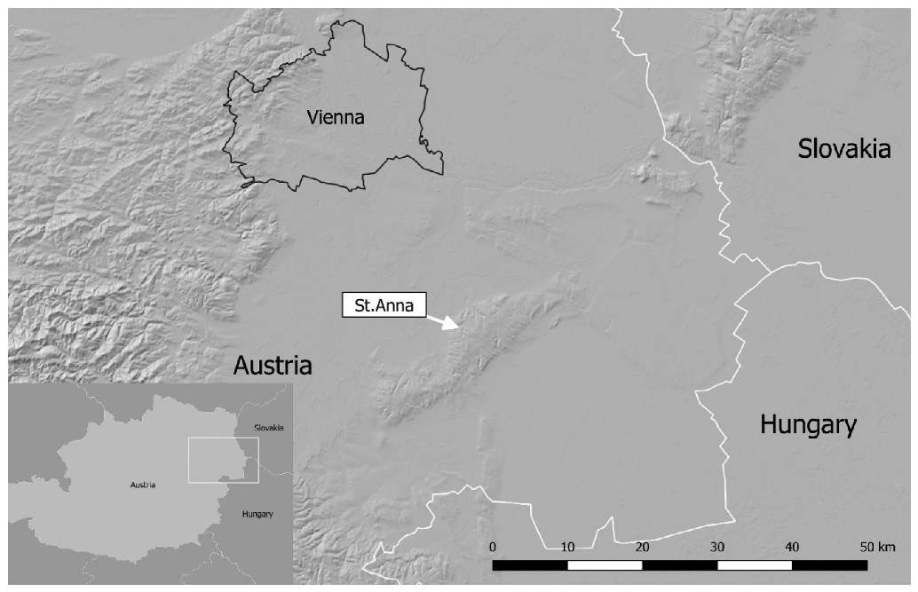
2. Case Study Area
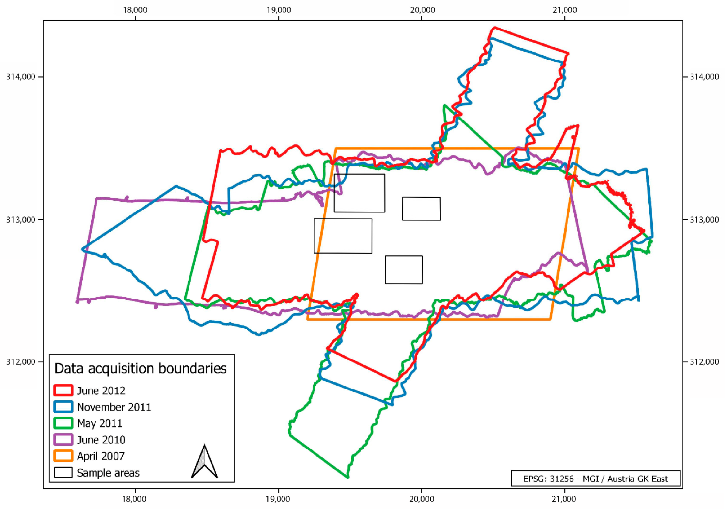
3. Data and Metadata
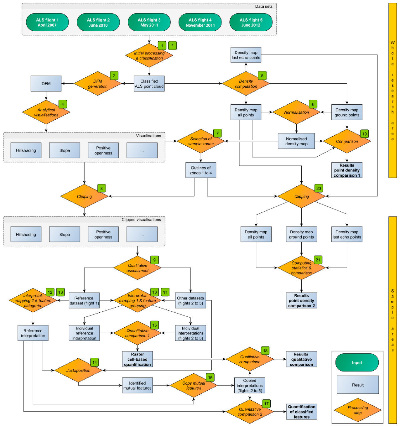
4. Methodology
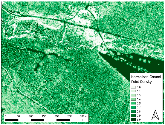
4.1. Point Cloud Processing and Density Maps
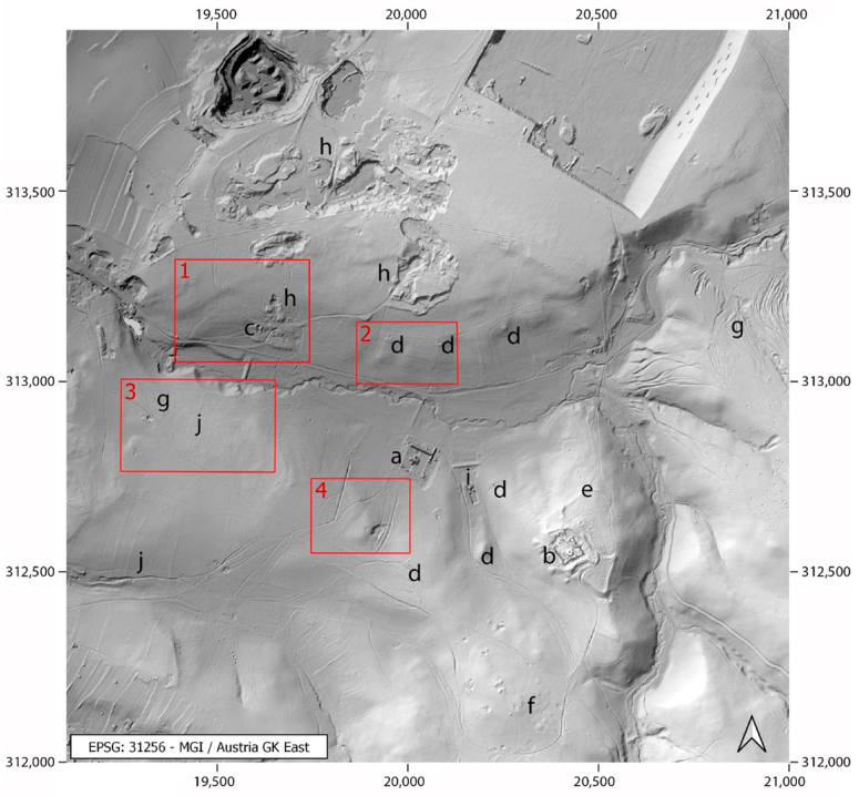
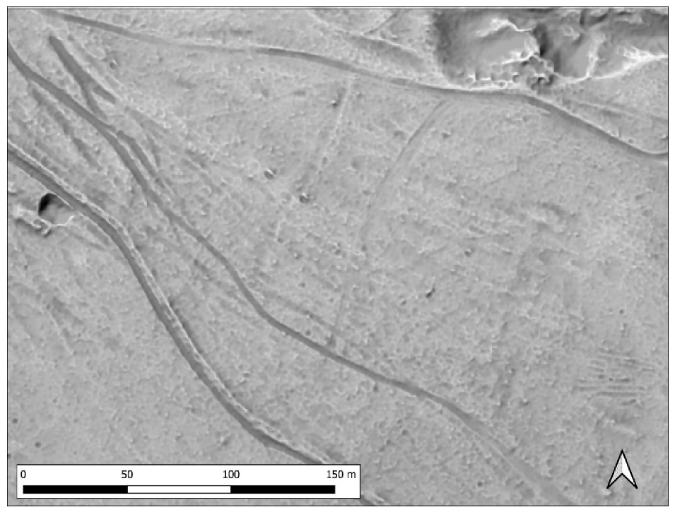
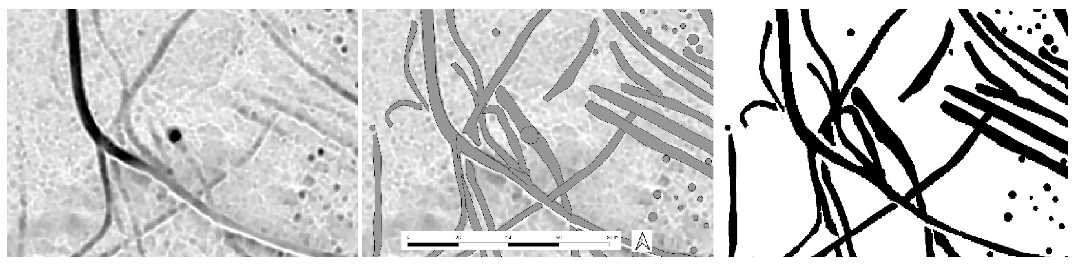
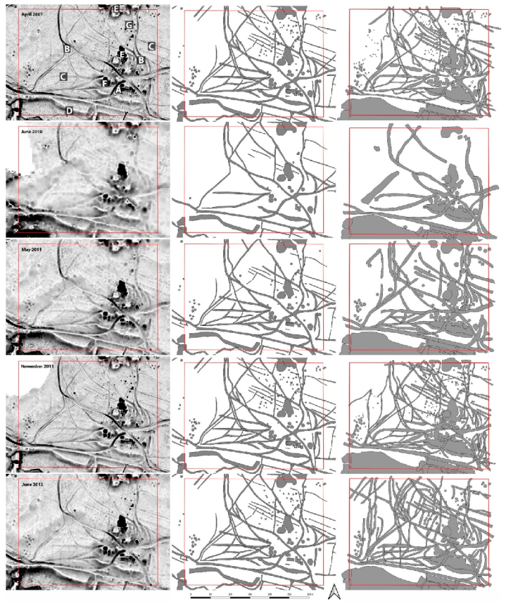
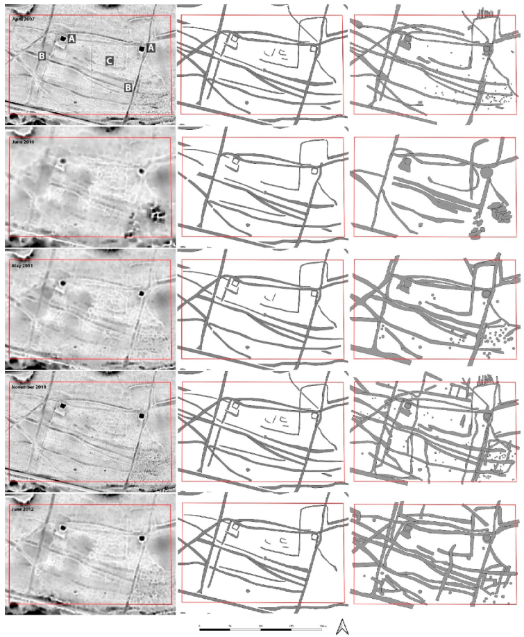
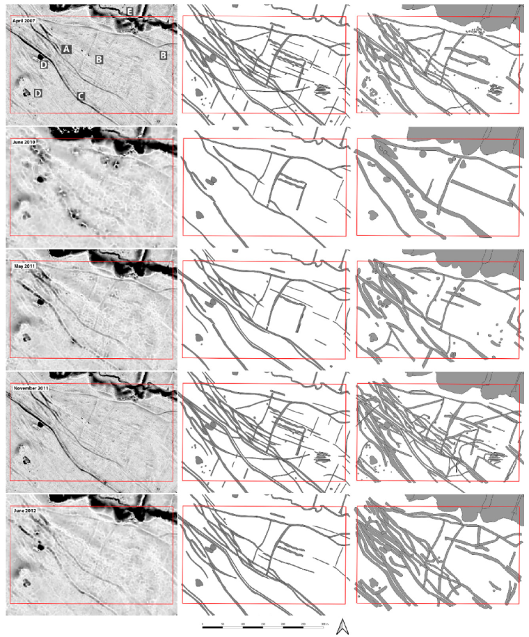
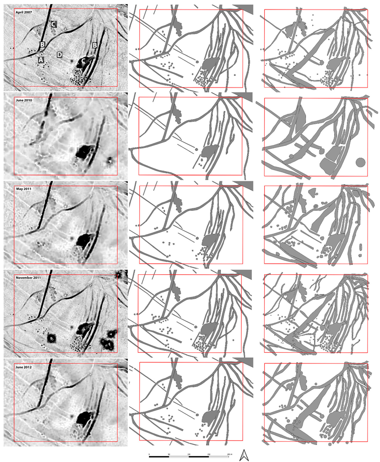
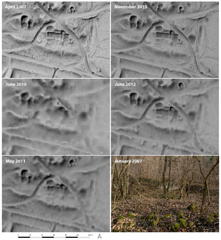
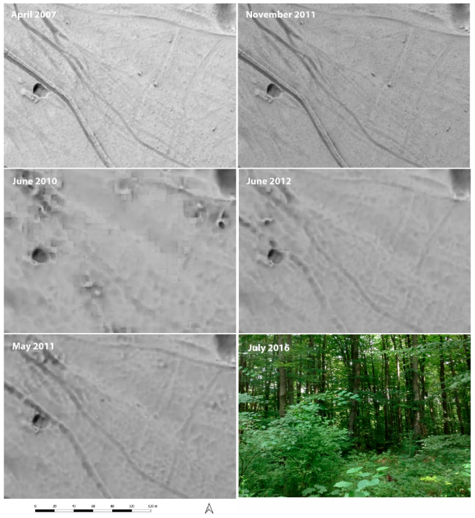
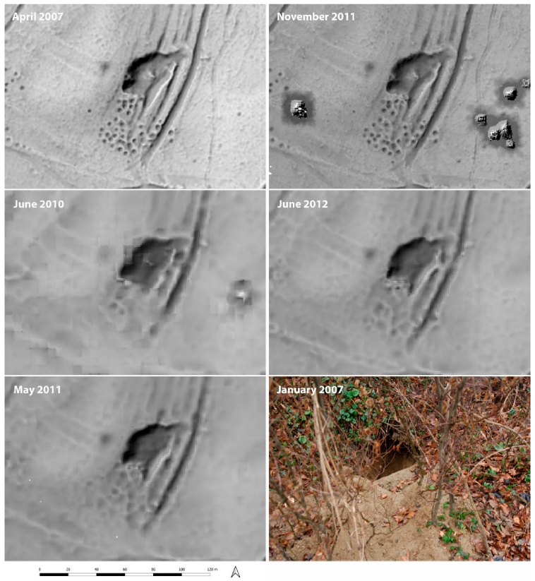
4.2. Interpretation of Sample Areas
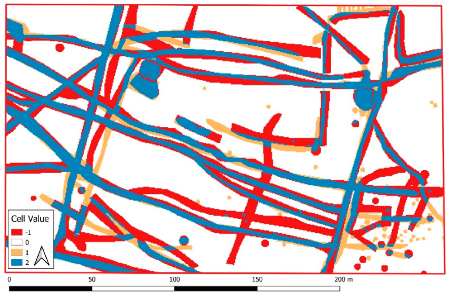
4.3. Comparing the Outputs of Interpretation
- ‘0’ represents no archaeological information (no features identified in any of the compared rasters) in both datasets;
- ‘1’ for features only detected in the reference raster (Spring 2007);
- ‘−1’ for features only detected in raster no. 2;
- ‘2’ for features detected in both rasters.
5. Results
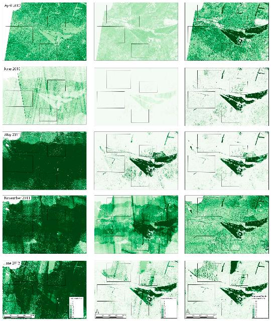
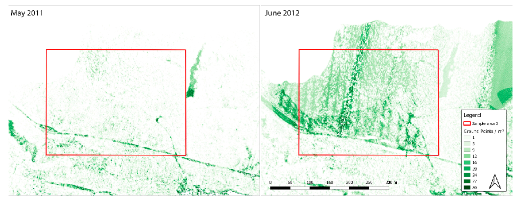
5.1. Point Density
5.2. Interpretation Results
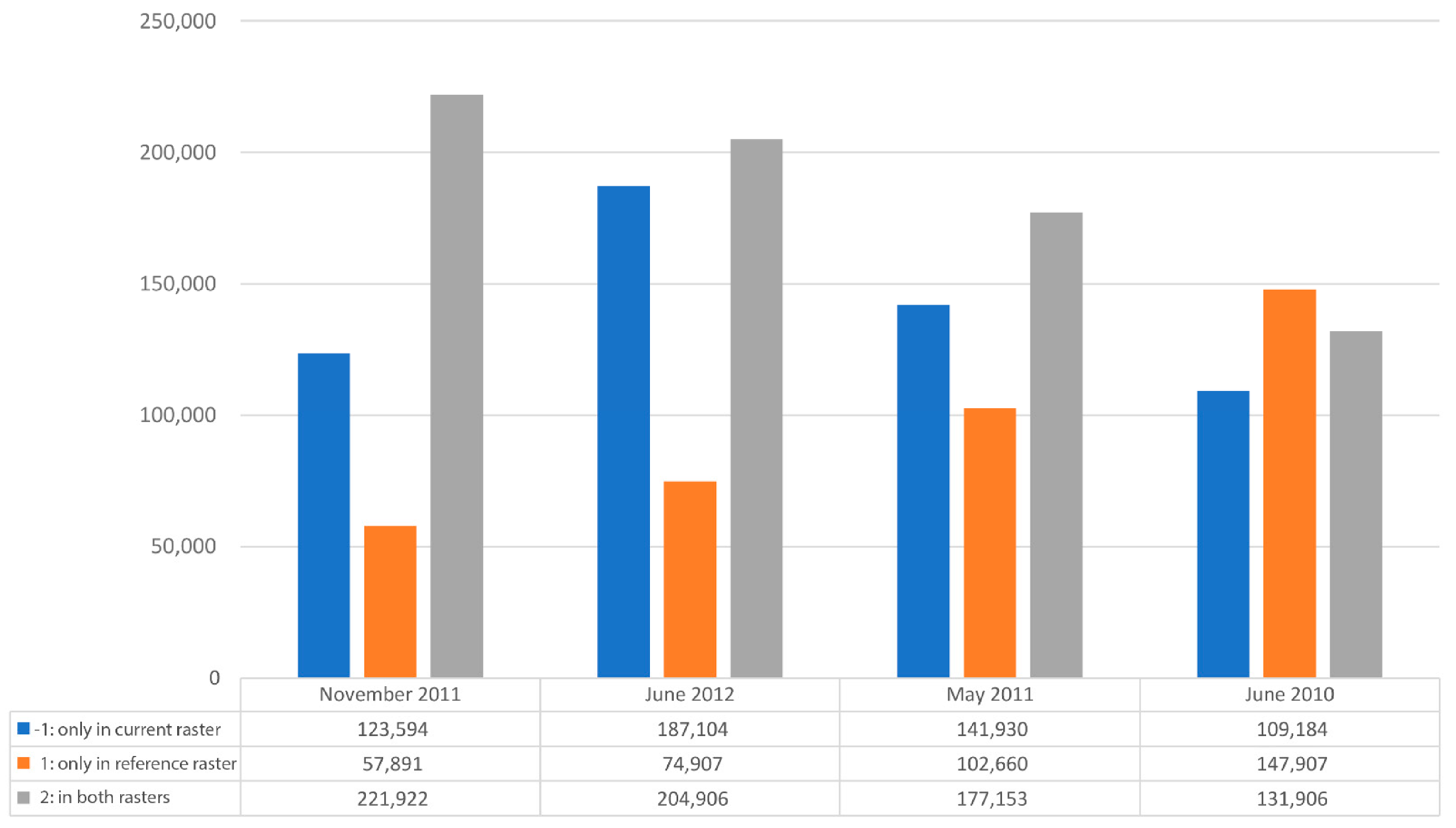
5.3. Quantitative Analysis
6. Discussion
6.1. Quantitative Approach
6.1.1. Comparison Based on Cell Values
6.1.2. Comparison Based on Discrete Features
6.2. Qualitative Approach
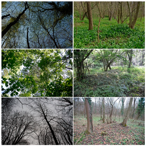
6.3. The Visibility of Archaeological Features
7. Conclusions
Author Contributions
Funding
Institutional Review Board Statement
Informed Consent Statement
Acknowledgments
Conflicts of Interest
References
- Doneus, M.; Briese, C. Digital terrain modelling for archaeological interpretation within forested areas using full-waveform laserscanning. In Proceedings of the 7th International Symposium on Virtual Reality, Archaeology and Cultural Heritage VAST, Nicosia, Cyprus, 30 October–4 November 2006; Ioannides, M., Arnold, D., Niccolucci, F., Mania, K., Eds.; pp. 155–162. [Google Scholar]
- Risbøl, O.; Gjertsen, K.A.; Skare, K. Airborne laser scanning of cultural remains in forests: Some preliminary results from a Norwegian project. In From Space to Place: 2. International Conference on Remote Sensing in Archaeology: Proceedings of the 2. International Workshop, CNR, Rome, Italy, 2–4 December 2006; Campana, S., Forte, M., Eds.; BAR International Series S1568; Archaeopress: Oxford, UK, 2006; pp. 107–112. ISBN 1 84171 998 6. [Google Scholar]
- Challis, K. Airborne laser altimetry in alluviated landscapes. Archaeol. Prospect. 2006, 13, 103–127. [Google Scholar] [CrossRef]
- Crutchley, S. Light detection and ranging (lidar) in the Witham Valley, Lincolnshire: An assessment of new remote sensing techniques. Archaeol. Prospect. 2006, 13, 251–257. [Google Scholar] [CrossRef]
- Crow, P.; Benham, S.; Devereux, B.; Amable, G. Woodland vegetation and its implications for archaeological survey using LiDAR. For. Int. J. For. Res. 2007, 80, 241–252. [Google Scholar] [CrossRef] [Green Version]
- Fernandez-Diaz, J.C.; Carter, W.E.; Shrestha, R.L.; Glennie, C.L. Now You See It… Now You Don’t: Understanding Airborne Mapping LiDAR Collection and Data Product Generation for Archaeological Research in Mesoamerica. Remote Sens. 2014, 6, 9951–10001. [Google Scholar] [CrossRef] [Green Version]
- Lozić, E.; Štular, B. Documentation of Archaeology-Specific Workflow for Airborne LiDAR Data Processing. Geosciences 2021, 11, 26. [Google Scholar] [CrossRef]
- Bofinger, J.; Hesse, R. As far as the laser can reach… Laminar analysis of LiDAR detected structures as a powerful instrument for archaeological heritage management in Baden-Württemberg, Germany. In Remote Sensing for Archaeological Heritage Management: Proceedings of the 11th EAC Heritage Management Symposium, Reykjavik, Iceland, 25–27 March 2010; Cowley, D., Ed.; Archaeolingua, EAC: Budapest, Hungary, 2011; pp. 161–171. ISBN 978-963-9911-20-8. [Google Scholar]
- Wroniecki, P.; Jaworski, M.; Kostyrko, M. Exploring free LiDAR derivatives. A user’s perspective on the potential of readily available resources in Poland. Archaeol. Pol. 2015, 53, 612–616. [Google Scholar]
- Banaszek, Ł.; Cowley, D.C.; Middleton, M. Towards National Archaeological Mapping. Assessing Source Data and Methodology—A Case Study from Scotland. Geosciences 2018, 8, 272. [Google Scholar] [CrossRef] [Green Version]
- Doneus, M.; Briese, C. Airborne Laser Scanning in Forested Areas—Potential and Limitations of an Archaeological Prospection Technique. In Remote Sensing for Archaeological Heritage Management: Proceedings of the 11th EAC Heritage Management Symposium, Reykjavik, Iceland, 25–27 March 2010; Cowley, D., Ed.; Archaeolingua, EAC: Budapest, Hungary, 2011; pp. 53–76. ISBN 978-963-9911-20-8. [Google Scholar]
- Banaszek, Ł. Przeszłe Krajobrazy w Chmurze Punktów; Wydawnictwo Naukowe UAM: Poznań, Poland, 2015. [Google Scholar]
- Klimczyk, A.; Doneus, M.; Briese, C.; Pfeifer, N. Evaluation of different software packages for ALS filtering. In Archaeological Prospection: Proceedings of the 10th International Conference–Vienna; Neubauer, W., Trinks, I., Salisbury, R.B., Einwögerer, C., Eds.; Verl. der Österr. Akad. d. Wiss.: Wien, Austria, 2013; pp. 363–366. ISBN 9783700174592. [Google Scholar]
- Kiarszys, G.; Szalast, G. Archeologia w chmurze punktów. Porównanie rezultatów filtracji i klasyfikacji gruntu w projekcie ISOK z wynikami opracowanymi w oprogramowaniu LAStools i Terrasolid. Folia Praehist. Posnaniensia 2014, 19, 267–292. [Google Scholar] [CrossRef]
- Banaszek, Ł. Lotniczy skaning laserowy w polskiej archeologii. Czy w pełni wykorzystywany jest potencjał prospekcyjny metody? Folia Praehist. Posnaniensia 2014, 19, 207. [Google Scholar] [CrossRef]
- Štular, B.; Lozić, E. Comparison of Filters for Archaeology-Specific Ground Extraction from Airborne LiDAR Point Clouds. Remote Sens. 2020, 12, 3025. [Google Scholar] [CrossRef]
- Doneus, M.; Mandlburger, G.; Doneus, N. Archaeological Ground Point Filtering of Airborne Laser Scan Derived Point-Clouds in a Difficult Mediterranean Environment. J. Comput. Appl. Archaeol. 2020, 3, 92–108. [Google Scholar] [CrossRef] [Green Version]
- Štular, B.; Lozić, E.; Eichert, S. Airborne LiDAR-Derived Digital Elevation Model for Archaeology. Remote Sens. 2021, 13, 1855. [Google Scholar] [CrossRef]
- Challis, K.; Forlin, P.; Kincey, M. A Generic Toolkit for the Visualization of Archaeological Features on Airborne LiDAR Elevation Data. Archaeol. Prospect. 2011, 18, 279–289. [Google Scholar] [CrossRef]
- Bennett, R.; Welham, K.; Hill, R.A.; Ford, A. A Comparison of Visualization Techniques for Models Created from Airborne Laser Scanned Data. Archaeol. Prospect. 2012, 19, 41–48. [Google Scholar] [CrossRef]
- Kokalj, Ž.; Somrak, M. Why Not a Single Image? Combining Visualizations to Facilitate Fieldwork and On-Screen Mapping. Remote. Sens. 2019, 11, 747. [Google Scholar] [CrossRef] [Green Version]
- Kokalj, Ž.; Zakšek, K.; Oštir, K.; Pehani, P.; Čotar, K.; Somrak, M. Relief Visualization Toolbox (RVT); Institute of Anthropological and Spatial Studies, ZRCSAZU: Ljubljana, Slovenia, 2020. [Google Scholar]
- Bradford, J. Ancient Landscapes: Studies in Field Archaeology; Bell & Sons: London, UK, 1957. [Google Scholar]
- Rączkowski, W. Theoretical dialogues–is there any theory in aerial archaeology? AARGNews 2005, 1, 12–22. [Google Scholar]
- Palmer, R. Knowledge-based aerial image interpretation. In Remote Sensing for Archaeological Heritage Management: Proceedings of the 11th EAC Heritage Management Symposium, Reykjavik, Iceland, 25–27 March 2010; Cowley, D., Ed.; Archaeolingua, EAC: Budapest, Hungary, 2011; pp. 283–291. ISBN 978-963-9911-20-8. [Google Scholar]
- Palmer, R. Reading aerial images. In Interpreting Archaeological Topography: Airborne Laser Scanning, 3D Data and Ground Observation; Opitz, R.S., Cowley, D., Eds.; Oxbow Books: Oxford, UK, 2013; pp. 76–87. ISBN 978-1-84217-516-3. [Google Scholar]
- Štular, B.; Eichert, S.; Lozić, E. Airborne LiDAR Point Cloud Processing for Archaeology. Pipeline and QGIS Toolbox. Remote Sens. 2021, 13, 3225. [Google Scholar] [CrossRef]
- White, J.C.; Arnett, J.T.; Wulder, M.A.; Tompalski, P.; Coops, N.C. Evaluating the impact of leaf-on and leaf-off airborne laser scanning data on the estimation of forest inventory attributes with the area-based approach. Can. J. For. Res. 2015, 45, 1498–1513. [Google Scholar] [CrossRef] [Green Version]
- Banaszek, Ł. The Past Amidst the Woods. The Post-Medieval Landscape of Polanów; Ad Rem: Poznań, Poland, 2019; ISBN 978-83-916342-6-4. [Google Scholar]
- Banaszek, Ł. It takes all kinds of trees to make a forest. Using historic maps and forestry data to inform airborne laser scanning based archaeological prospection in woodland. Archaeol. Prospect. 2020, 27, 377–392. [Google Scholar] [CrossRef]
- Chase, A.F.; Chase, D.Z.; Weishampel, J.F. Lasers in the Jungle: Airborne sensors reveal a vast Maya landscape. Archaeology 2010, 63, 27–29. [Google Scholar]
- Chase, A.F.; Chase, D.Z.; Weishampel, J.F.; Drake, J.B.; Shrestha, R.L.; Slatton, K.C.; Awe, J.J.; Carter, W.E. Airborne LiDAR, archaeology, and the ancient Maya landscape at Caracol, Belize. J. Archaeol. Sci. 2011, 38, 387–398. [Google Scholar] [CrossRef]
- Chase, A.F.; Chase, D.Z.; Fisher, C.T.; Leisz, S.J.; Weishampel, J.F. Geospatial revolution and remote sensing LiDAR in Mesoamerican archaeology. Proc. Natl. Acad. Sci. USA 2012, 109, 12916–12921. [Google Scholar] [CrossRef] [Green Version]
- Beach, T.; Luzzadder-Beach, S.; Krause, S.; Guderjan, T.; Valdez, F.; Fernandez-Diaz, J.C.; Eshleman, S.; Doyle, C. Ancient Maya wetland fields revealed under tropical forest canopy from laser scanning and multiproxy evidence. Proc. Natl. Acad. Sci. USA 2019, 116, 21469–21477. [Google Scholar] [CrossRef] [Green Version]
- Chevance, J.-B.; Evans, D.; Hofer, N.; Sakhoeun, S.; Chhean, R. Mahendraparvata: An early Angkor-period capital defined through airborne laser scanning at Phnom Kulen. Antiquity 2019, 93, 1303–1321. [Google Scholar] [CrossRef] [Green Version]
- Canuto, M.A.; Estrada-Belli, F.; Garrison, T.G.; Houston, S.D.; Acuña, M.J.; Kováč, M.; Marken, D.; Nondédéo, P.; Auld-Thomas, L.; Castanet, C.; et al. Ancient lowland Maya complexity as revealed by airborne laser scanning of northern Guatemala. Science 2018, 361, eaau0137. [Google Scholar] [CrossRef] [Green Version]
- Evans, D. Airborne laser scanning as a method for exploring long-term socio-ecological dynamics in Cambodia. J. Archaeol. Sci. 2016, 74, 164–175. [Google Scholar] [CrossRef] [Green Version]
- Cap, B.; Yaeger, J.; Brown, M.K. Fidelity tests of LiDAR data for the detection of ancient Maya settlement in the Upper Belize River Valley, Belize. Res. Rep. Belizean Archaeol. 2018, 15, 39–51. [Google Scholar]
- Doneus, M.; Briese, C.; Fera, M.; Janner, M. Archaeological prospection of forested areas using full-waveform airborne laser scanning. J. Archaeol. Sci. 2008, 35, 882–893. [Google Scholar] [CrossRef]
- Doneus, M.; Briese, C.; Kühtreiber, T. Flugzeuggetragenes Laserscanning als Werkzeug der archäologischen Kulturlandschaftsforschung. Das Fallbeispiel “Wüste” bei Mannersdorf am Leithagebirge, Niederösterreich. Archäologisches Korresp. 2008, 38, 137–156. [Google Scholar]
- Doneus, M.; Briese, C.; Studnicka, N. Analysis of Full-Waveform ALS Data by Simultaneously Acquired TLS Data: Towards an Advanced DTM Generation in Wooded Ar. In Proceedings of the 100 Years ISPRS, Advancing Remote Sensing Science: ISPRS Technical Commission VII Symposium, Vienna, Austria, 5–7 July 2010; pp. 193–198. [Google Scholar]
- Doneus, M.; Kühtreiber, T. Airborne laser scanning and archaeological interpretation–bringing back the people. In Interpreting Archaeological Topography: Airborne Laser Scanning, 3D Data and Ground Observation; Opitz, R.S., Cowley, D., Eds.; Oxbow Books: Oxford, UK, 2013; pp. 32–50. ISBN 978-1-84217-516-3. [Google Scholar]
- Doneus, M. Openness as Visualization Technique for Interpretative Mapping of Airborne Lidar Derived Digital Terrain Models. Remote Sens. 2013, 5, 6427–6442. [Google Scholar] [CrossRef] [Green Version]
- Trinks, I.; Neubauer, W.; Doneus, M. Prospecting Archaeological Landscapes. In Progress in Cultural Heritage Preservation: 4th International Conference, EuroMed 2012, Limassol, Cyprus, 29 October–3 November 2012; Ioannides, M., Fritsch, D., Leissner, J., Davies, R., Remondino, F., Caffo, R., Eds.; Springer: Berlin/Heidelberg, Germany, 2012; pp. 21–29. ISBN 978-3-642-34234-9_3. [Google Scholar]
- Mandlburger, G.; Otepka, J.; Karel, W.; Wagner, W.; Pfeifer, N. Orientation and Processing of Airborne Laser Scanning data (OPALS)–concept and first results of a comprehensive ALS software. In Proceedings of the ISPRS Workshop Laserscanning ’09, Paris, France, 1–2 September 2009; Bretar, F., Pierrot-Deseilligny, M., Vosselman, G., Eds.; Société Française de Photogrammétrie et de Télédétection: Marne-la-Vallée, France, 2009. [Google Scholar]
- Pfeifer, N.; Mandlburger, G.; Otepka, J.; Karel, W. OPALS–A framework for Airborne Laser Scanning data analysis. Comput. Environ. Urban Syst. 2014, 45, 125–136. [Google Scholar] [CrossRef]
- Pingel, T.J.; Clarke, K.; Ford, A. Bonemapping: A LiDAR processing and visualization technique in support of archaeology under the canopy. Cartogr. Geogr. Inf. Sci. 2015, 42, 18–26. [Google Scholar] [CrossRef]
- Kraus, K. Interpolation nach kleinsten Quadraten versus Krige-Schätzer. Österr. Zeitschr. Vermess. Geoinf. 1998, 86, 45–48. [Google Scholar]
- Bollandsås, O.; Risbøl, O.; Ene, L.; Nesbakken, A.; Gobakken, T.; Næsset, E. Using airborne small-footprint laser scanner data for detection of cultural remains in forests: An experimental study of the effects of pulse density and DTM smoothing. J. Archaeol. Sci. 2012, 39, 2733–2743. [Google Scholar] [CrossRef]
- Norstedt, G.; Axelsson, A.-L.; Laudon, H.; Östlund, L. Detecting Cultural Remains in Boreal Forests in Sweden Using Airborne Laser Scanning Data of Different Resolutions. J. Field Archaeol. 2020, 45, 16–28. [Google Scholar] [CrossRef]
- Doneus, M.; Shinoto, M.; Herzog, I.; Nakamura, N.; Haijima, H.; Ōnishi, T.; Kita’ichi, S.; Song, B. UAV-based Airborne Laser Scanning in densely vegetated areas: Detecting Sue pottery kilns in Nakadake Sanroku, Japan. New Global Perspectives on Archaeological Prospection. In Proceedings of the 13th International Conference On Archaeological Prospection, Sligo, Ireland, 28 August–1 September 2019; Bonsall, J., Ed.; Archaeopress: Oxford, UK, 2019; pp. 220–223, ISBN 978-1-78969-306-5. [Google Scholar]
- Campana, S. Drones in Archaeology. State-of-the-art and Future Perspectives. Archaeol. Prospect. 2017, 24, 275–296. [Google Scholar] [CrossRef]
- Risbøl, O.; Gustavsen, L. LiDAR from drones employed for mapping archaeology–Potential, benefits and challenges. Archaeol. Prospect. 2018, 25, 329–338. [Google Scholar] [CrossRef]


| ALS-Project | Leithagebirge | LBI ArchPro—St. Anna | LBI ArchPro—St. Anna | LBI ArchPro—St. Anna | LBI ArchPro—St. Anna |
|---|---|---|---|---|---|
| Purpose of scan | Archaeology | Archaeology (spectroscopy) | Archaeology | Archaeology | Archaeology |
| Time of data acquisition | 26 March–12 April 2007 | 9 June 2010 | 26 May 2011 | 11 November 2011 | 18 June 2012 |
| Mean point density of return (all echoes) per m2 | 17 | 5 | 33.5 | 21.5 | 25.7 |
| Mean point density of last echoes per m2 | 9.7 | 3 | 22.8 | 13.1 | 15.1 |
| Ground points (after filtering) per m2 | 5.4 | 0.5 | 1.5 | 4.4 | 2.2 |
| Strip overlap | 70% | 70% | 70% | 70% | 70% |
| Scanner type | Riegl LMS-Q560 Full-Waveform | Riegl LMS-Q680i Full-Waveform | Riegl LMS-Q680i Full-Waveform | Riegl LMS-Q680i Full-Waveform | Riegl LMS-Q680i Full-Waveform |
| Scan angle (whole FOV) | 45° | 60° | 60° | 60° | 60° |
| Flying height above ground | 600 m | 450 m | 450 m | 450 m | 450 m |
| Speed of aircraft (TAS) | 70 kts (36 m/s) | 98 kts (50 m/s) | 98 kts (50 m/s) | 98 kts (50 m/s) | 98 kts (50 m/s) |
| Laser pulse rate | 100,000 Hz | 400,000 Hz | 400,000 Hz | 400,000 Hz | 400,000 Hz |
| Scan rate | 66,000 Hz | 140,000 Hz | 400,000 Hz | 400,000 Hz | 400,000 Hz |
| Strip adjustment | Yes | Yes | Yes | Yes | Yes |
| Filtering | Robust interpolation (OPALS) | Robust interpolation (OPALS) | Robust interpolation (OPALS) | Robust interpolation (OPALS) | Robust interpolation (OPALS) |
| DTM cell size | 0.5 m | 1 m | 0.5 m | 0.5 m | 0.5 m |
| Category | Spring 2007 | June 2010 | May 2011 | Nov. 11 | June 2012 | ||||||
|---|---|---|---|---|---|---|---|---|---|---|---|
| Pt/m2 | % | Pt/m2 | % | Pt/m2 | % | Pt/m2 | % | Pt/m2 | % | ||
| Area 1 | Ground points | 6.2 | 38 | 0.3 | 4 | 1.3 | 3 | 10.9 | 37 | 5.6 | 18 |
| Last echoes | 9.6 | 59 | 3.8 | 55 | 23.8 | 58 | 14.8 | 50 | 15.9 | 50 | |
| All echoes | 16.2 | 100 | 6.9 | 100 | 40.8 | 100 | 29.6 | 100 | 31.4 | 100 | |
| Area 2 | Ground points | 8.1 | 49 | 0.7 | 7 | 4.8 | 6 | 21.7 | 41 | 7.7 | 12 |
| Last echoes | 9.8 | 59 | 4.4 | 46 | 47 | 58 | 26.2 | 49 | 29.9 | 48 | |
| All echoes | 16.7 | 100 | 9.6 | 100 | 81.3 | 100 | 53.4 | 100 | 62.6 | 100 | |
| Area 3 | Ground points | 7.2 | 48 | 0.3 | 4 | 2.3 | 3 | 17.9 | 35 | 1.8 | 4 |
| Last echoes | 9.7 | 64 | 3.6 | 54 | 44.9 | 63 | 24.2 | 47 | 23.1 | 57 | |
| All echoes | 15.1 | 100 | 6.7 | 100 | 71.3 | 100 | 51.2 | 100 | 40.2 | 100 | |
| Area 4 | Ground points | 8.3 | 53 | 0.5 | 7 | 4 | 6 | 14.7 | 34 | 3.9 | 7 |
| Last echoes | 9.9 | 63 | 3.8 | 53 | 42.8 | 63 | 21.2 | 50 | 30.1 | 53 | |
| All echoes | 15.8 | 100 | 7.2 | 100 | 69.3 | 100 | 42.8 | 100 | 56.8 | 100 | |
| Average | Ground points | 7.45 | 47 | 0.45 | 5.5 | 3.1 | 4.5 | 16.3 | 36.75 | 4.75 | 10.25 |
| Last echoes | 9.75 | 61.25 | 3.9 | 52 | 39.625 | 60.5 | 21.6 | 49 | 24.75 | 52 | |
| All echoes | 15.95 | 100 | 7.6 | 100 | 65.675 | 100 | 44.25 | 100 | 47.75 | 100 | |
| Cell Value | June 2010 | May 2011 | November 2011 | June 2012 | |||||||||
|---|---|---|---|---|---|---|---|---|---|---|---|---|---|
| Linear Features | Pits | Total | Linear Features | Pits | Total | Linear Features | Pits | Total | Linear Features | Pits | Total | ||
| Area 1 | −1 | 29.7 | 2.6 | 32.4 | 47.0 | 7.9 | 54.9 | 34.1 | 3.2 | 37.3 | 60.3 | 4.9 | 65.3 |
| 1 | 45.0 | 9.1 | 54.2 | 25.8 | 6.6 | 32.3 | 17.3 | 3.6 | 20.9 | 21.4 | 5.3 | 26.7 | |
| 2 | 39.3 | 7.4 | 46.8 | 58.6 | 10.0 | 68.6 | 67.0 | 13.0 | 80.0 | 63.0 | 11.3 | 74.2 | |
| Area 2 | −1 | 13.6 | 3.1 | 16.7 | 19.1 | 2.0 | 21.1 | 19.7 | 0.9 | 20.6 | 27.5 | 1.1 | 28.7 |
| 1 | 20.2 | 8.7 | 21.1 | 11.5 | 0.8 | 12.2 | 5.3 | 0.6 | 6.0 | 6.8 | 0.9 | 7.7 | |
| 2 | 16.8 | 1.3 | 16.9 | 25.5 | 0.2 | 25.7 | 31.6 | 0.4 | 32.0 | 30.1 | 0.1 | 30.3 | |
| Area 3 | −1 | 28.4 | 1.9 | 30.4 | 31.2 | 2.3 | 33.5 | 42.0 | 0.7 | 42.8 | 60.4 | 1.5 | 61.8 |
| 1 | 49.0 | 2.7 | 51.8 | 37.4 | 2.6 | 40.0 | 18.9 | 2.1 | 21.1 | 25.8 | 2.6 | 28.4 | |
| 2 | 28.7 | 1.5 | 30.2 | 40.4 | 1.6 | 42.0 | 58.8 | 2.1 | 60.9 | 51.9 | 1.6 | 53.5 | |
| Area 4 | −1 | 23.0 | 6.7 | 29.7 | 25.9 | 6.4 | 32.4 | 21.4 | 1.5 | 22.9 | 28.2 | 3.2 | 31.3 |
| 1 | 16.5 | 4.3 | 20.8 | 13.7 | 4.4 | 18.1 | 7.6 | 2.4 | 10.0 | 8.1 | 3.9 | 12.0 | |
| 2 | 30.5 | 7.6 | 38.1 | 33.4 | 7.5 | 40.9 | 39.5 | 9.5 | 49.0 | 39.0 | 8.0 | 46.9 | |
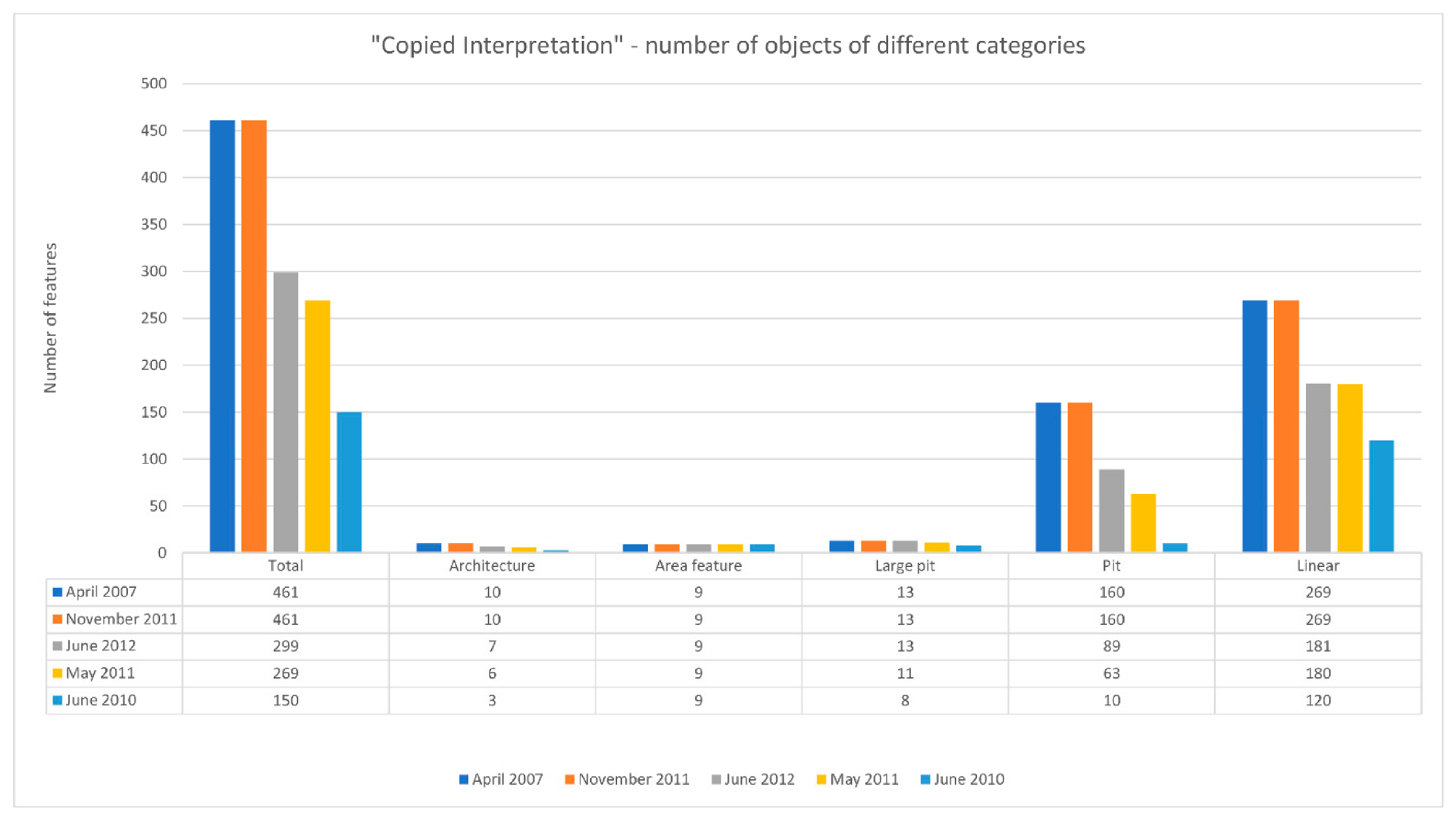
| Dataset | Architecture | Area Feature | Large Pit | Pit | Linear | Total | |
|---|---|---|---|---|---|---|---|
| Area 1 | 2007 April | 8 | 4 | 12 | 76 | 72 | 172 |
| 2010 June | 1 | 4 | 7 | 5 | 36 | 53 | |
| 2011 May | 4 | 4 | 10 | 29 | 60 | 107 | |
| 2011 November | 8 | 4 | 12 | 76 | 72 | 172 | |
| 2012 June | 5 | 4 | 12 | 57 | 66 | 144 | |
| Area 2 | 2007 April | 2 | 0 | 0 | 2 | 48 | 52 |
| 2010 June | 2 | 0 | 0 | 2 | 31 | 35 | |
| 2011 May | 2 | 0 | 0 | 2 | 40 | 44 | |
| 2011 November | 2 | 0 | 0 | 2 | 48 | 52 | |
| 2012 June | 2 | 0 | 0 | 2 | 38 | 42 | |
| Area 3 | 2007 April | 0 | 3 | 0 | 16 | 105 | 124 |
| 2010 June | 0 | 3 | 0 | 0 | 24 | 27 | |
| 2011 May | 0 | 3 | 0 | 4 | 47 | 54 | |
| 2011 November | 0 | 3 | 0 | 16 | 105 | 124 | |
| 2012 June | 0 | 3 | 0 | 1 | 47 | 51 | |
| Area 4 | 2007 April | 0 | 2 | 1 | 66 | 44 | 113 |
| 2010 June | 0 | 2 | 1 | 3 | 29 | 35 | |
| 2011 May | 0 | 2 | 1 | 28 | 33 | 64 | |
| 2011 November | 0 | 2 | 1 | 66 | 44 | 113 | |
| 2012 June | 0 | 2 | 1 | 29 | 30 | 62 |
Publisher’s Note: MDPI stays neutral with regard to jurisdictional claims in published maps and institutional affiliations. |
© 2022 by the authors. Licensee MDPI, Basel, Switzerland. This article is an open access article distributed under the terms and conditions of the Creative Commons Attribution (CC BY) license (https://creativecommons.org/licenses/by/4.0/).
Share and Cite
Doneus, M.; Banaszek, Ł.; Verhoeven, G.J. The Impact of Vegetation on the Visibility of Archaeological Features in Airborne Laser Scanning Datasets from Different Acquisition Dates. Remote Sens. 2022, 14, 858. https://0-doi-org.brum.beds.ac.uk/10.3390/rs14040858
Doneus M, Banaszek Ł, Verhoeven GJ. The Impact of Vegetation on the Visibility of Archaeological Features in Airborne Laser Scanning Datasets from Different Acquisition Dates. Remote Sensing. 2022; 14(4):858. https://0-doi-org.brum.beds.ac.uk/10.3390/rs14040858
Chicago/Turabian StyleDoneus, Michael, Łukasz Banaszek, and Geert J. Verhoeven. 2022. "The Impact of Vegetation on the Visibility of Archaeological Features in Airborne Laser Scanning Datasets from Different Acquisition Dates" Remote Sensing 14, no. 4: 858. https://0-doi-org.brum.beds.ac.uk/10.3390/rs14040858