
A New Adaptive Remote Sensing Extraction Algorithm for Complex Muddy Coast Waterline

 , , , and
Abstract
:
1. Introduction
2. Materials and Methods
2.1. Study Area
2.2. Data Source
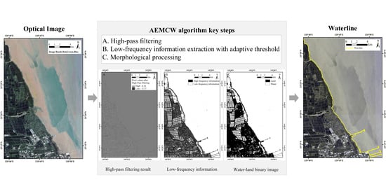
2.3. Methodology
2.3.1. The Pre-Processing of Remote Sensing Image
2.3.2. The Selection of the Best Band
2.3.3. Low-Frequency Information Extraction
- (a)
- High-pass filtering
- (b) Histogram statistics
- (c) Adaptive threshold determination
2.3.4. Morphological Processing
2.3.5. Post-Processing
2.3.6. Accuracy Assessment
3. Results
3.1. The Best Band to Extract Waterline
3.2. Waterline Extraction Results of Muddy Coast
4. Discussion
4.1. Accuracy Assessment
4.1.1. Threshold Settings and Extraction Results
4.1.2. Length Accuracy Analysis
4.1.3. Spatial Accuracy Analysis
4.2. Application of Proposed Method in Hyperspectral Image
5. Conclusions
Author Contributions
Funding
Institutional Review Board Statement
Informed Consent Statement
Data Availability Statement
Acknowledgments
Conflicts of Interest
References
- Ma, X.; Zhao, K.; Li, Y.; Zhu, H. Infrastructure Investment and Sustainable Development in Coastal Areas in China. J. Coast. Res. 2019, 94, 67–72. [Google Scholar] [CrossRef]
- Primavera, J. Overcoming the impacts of aquaculture on the coastal zone. Ocean Coast. Manag. 2006, 49, 531–545. [Google Scholar] [CrossRef]
- Trinh, L.H.; Le, T.G.; Kieu, V.H.; Tran, T.M.L.; Nguyen, T.T.N. Application of remote sensing technique for shoreline change detection in Ninh Binh and Nam Dinh provinces (Vietnam) during the period 1988 to 2018 based on water indices. Russ. J. Earth Sci. 2020, 20, 1–15. [Google Scholar] [CrossRef] [Green Version]
- Xu, N. Detecting Coastline Change with All Available Landsat Data over 1986–2015: A Case Study for the State of Texas, USA. Atmosphere 2018, 9, 107. [Google Scholar] [CrossRef] [Green Version]
- Toure, S.; Diop, O.; Kpalma, K.; Maiga, A.S. Shoreline Detection using Optical Remote Sensing: A Review. ISPRS Int. J. Geo-Information 2019, 8, 75. [Google Scholar] [CrossRef] [Green Version]
- Bishop-Taylor, R.; Sagar, S.; Lymburner, L.; Alam, I.; Sixsmith, J. Sub-Pixel Waterline Extraction: Characterising Accuracy and Sensitivity to Indices and Spectra. Remote Sens. 2019, 11, 2984. [Google Scholar] [CrossRef] [Green Version]
- Zhang, T.; Yang, X.; Hu, S.; Su, F. Extraction of Coastline in Aquaculture Coast from Multispectral Remote Sensing Images: Object-Based Region Growing Integrating Edge Detection. Remote Sens. 2013, 5, 4470–4487. [Google Scholar] [CrossRef] [Green Version]
- Tong, S.S.; Deroin, J.P.; Pham, T.L. An optimal waterline approach for studying tidal flat morphological changes using remote sensing data: A case of the northern coast of Vietnam. Estuar. Coast. Shelf Sci. 2020, 236, 106613. [Google Scholar] [CrossRef]
- Han-Qiu, X.U. A Study on Information Extraction of Water Body with the Modified Normalized Difference Water Index (MNDWI). J. Remote Sens. 2005, 9, 589–595. [Google Scholar] [CrossRef]
- Sagar, S.; Roberts, D.; Bala, B.; Lymburner, L. Extracting the intertidal extent and topography of the Australian coastline from a 28 year time series of Landsat observations. Remote Sens. Environ. 2017, 195, 153–169. [Google Scholar] [CrossRef]
- Bai, J.; Chen, X.; Li, J.; Yang, L.; Fang, H. Changes in the area of inland lakes in arid regions of central Asia during the past 30 years. Environ. Monit. Assess. 2011, 178, 247–256. [Google Scholar] [CrossRef] [PubMed]
- Yang, X.; Lu, X.X. Drastic change in China’s lakes and reservoirs over the past decades. Sci. Rep. 2015, 4, srep06041. [Google Scholar] [CrossRef] [PubMed] [Green Version]
- Li, Z.; Heygster, G.; Notholt, J. Intertidal Topographic Maps and Morphological Changes in the German Wadden Sea between 1996–1999 and 2006–2009 from the Waterline Method and SAR Images. IEEE J. Sel. Top. Appl. Earth Obs. Remote Sens. 2014, 7, 3210–3224. [Google Scholar] [CrossRef]
- Zhu, Z.; Tang, Y.; Hu, J.; An, M. Coastline Extraction From High-Resolution Multispectral Images by Integrating Prior Edge Information With Active Contour Model. IEEE J. Sel. Top. Appl. Earth Obs. Remote Sens. 2019, 12, 4099–4109. [Google Scholar] [CrossRef]
- Wang, D.; Liu, X. Coastline Extraction from SAR Images Using Robust Ridge Tracing. Mar. Geodesy 2019, 42, 286–315. [Google Scholar] [CrossRef]
- Pardo-Pascual, J.E.; Almonacid-Caballer, J.; Ruiz, L.A.; Palomar-Vazquez, J. Automatic extraction of shorelines from Landsat TM and ETM+ multi-temporal images with subpixel precision. Remote Sens. Environ. 2012, 123, 1–11. [Google Scholar] [CrossRef] [Green Version]
- Liu, H.; Jezek, K.C. Automated extraction of coastline from satellite imagery by integrating Canny edge detection and locally adaptive thresholding methods. Int. J. Remote Sens. 2004, 25, 937–958. [Google Scholar] [CrossRef]
- Ryu, J.-H.; Won, J.-S.; Min, K.D. Waterline extraction from Landsat TM data in a tidal flat: A case study in Gomso Bay, Korea. Remote Sens. Environ. 2002, 83, 442–456. [Google Scholar] [CrossRef]
- Zhang, X.; Zhou, C.-X.; Dong-Chen, E.; An, J.-C. Monitoring the change of Antarctic ice shelves and coastline based on multiple-source remote sensing data. Chin. J. Geophys. 2013, 56, 3302–3312. [Google Scholar]
- Su, H.; Wang, Y.; Yang, J. Monitoring the Spatiotemporal Evolution of Sea Ice in the Bohai Sea in the 2009–2010 Winter Combining MODIS and Meteorological Data. Estuaries Coasts 2011, 35, 281–291. [Google Scholar] [CrossRef] [Green Version]
- Rigos, A.; Tsekouras, G.E.; Vousdoukas, M.I.; Chatzipavlis, A.; Velegrakis, A.F. A Chebyshev polynomial radial basis function neural network for automated shoreline extraction from coastal imagery. Integr. Comput. Eng. 2016, 23, 141–160. [Google Scholar] [CrossRef] [Green Version]
- Mueller, N.; Lewis, A.; Roberts, D.; Ring, S.; Melrose, R.; Sixsmith, J.; Lymburner, L.; McIntyre, A.; Tan, P.; Curnow, S.; et al. Water observations from space: Mapping surface water from 25 years of Landsat imagery across Australia. Remote Sens. Environ. 2016, 174, 341–352. [Google Scholar] [CrossRef] [Green Version]
- Pekel, J.-F.; Cottam, A.; Gorelick, N.; Belward, A.S. High-resolution mapping of global surface water and its long-term changes. Nature 2016, 540, 418–422. [Google Scholar] [CrossRef] [PubMed]
- Tulbure, M.G.; Broich, M.; Stehman, S.V.; Kommareddy, A. Surface water extent dynamics from three decades of seasonally continuous Landsat time series at subcontinental scale in a semi-arid region. Remote Sens. Environ. 2016, 178, 142–157. [Google Scholar] [CrossRef]
- Sánchez-García, E.; Palomar-Vázquez, J.; Pardo-Pascual, J.; Almonacid-Caballer, J.; Cabezas-Rabadán, C.; Gómez-Pujol, L. An efficient protocol for accurate and massive shoreline definition from mid-resolution satellite imagery. Coast. Eng. 2020, 160, 103732. [Google Scholar] [CrossRef]
- Hong, Z.; Li, X.; Han, Y.; Zhang, Y.; Wang, J.; Zhou, R.; Hu, K. Automatic sub-pixel coastline extraction based on spectral mixture analysis using EO-1 Hyperion data. Front. Earth Sci. 2019, 13, 478–494. [Google Scholar] [CrossRef]
- Sánchez-García, E.; Balaguer-Beser, Á.; Almonacid-Caballer, J.; Pardo-Pascual, J.E. A New Adaptive Image Interpolation Method to Define the Shoreline at Sub-Pixel Level. Remote Sens. 2019, 11, 1880. [Google Scholar] [CrossRef] [Green Version]
- Vos, K.; Harley, M.D.; Splinter, K.D.; Simmons, J.A.; Turner, I.L. Sub-annual to multi-decadal shoreline variability from publicly available satellite imagery. Coast. Eng. 2019, 150, 160–174. [Google Scholar] [CrossRef]
- Vos, K.; Splinter, K.D.; Harley, M.; Simmons, J.A.; Turner, I.L. CoastSat: A Google Earth Engine-enabled Python toolkit to extract shorelines from publicly available satellite imagery. Environ. Model. Softw. 2019, 122, 104528. [Google Scholar] [CrossRef]
- Kuleli, T.; Guneroglu, A.; Karsli, F.; Dihkan, M. Automatic detection of shoreline change on coastal Ramsar wetlands of Turkey. Ocean Eng. 2011, 38, 1141–1149. [Google Scholar] [CrossRef]
- Cheng, D.; Meng, G.; Cheng, G.; Pan, C. SeNet: Structured Edge Network for Sea–Land Segmentation. IEEE Geosci. Remote Sens. Lett. 2016, 14, 247–251. [Google Scholar] [CrossRef]
- Liu, X.-Y.; Jia, R.-S.; Liu, Q.-M.; Zhao, C.-Y.; Sun, H.-M. Coastline Extraction Method Based on Convolutional Neural Networks—A Case Study of Jiaozhou Bay in Qingdao, China. IEEE Access 2019, 7, 180281–180291. [Google Scholar] [CrossRef]
- Chan, F.; Lam, F.; Zhu, H. Adaptive thresholding by variational method. IEEE Trans. Image Process. 1998, 7, 468–473. [Google Scholar] [CrossRef] [Green Version]
- Wei, L.-X.; Yang, B.; Jiang, J.-P.; Cao, G.-Z. Adaptive algorithm for classifying LiDAR data into water and land points by multifeature statistics. J. Appl. Remote Sens. 2016, 10, 45020. [Google Scholar] [CrossRef]
- Liang, L.; Liu, Q.S.; Liu, G.H.; Li, X.Y.; Huang, C. Review of Coastline Extraction Methods Based on Remote Sensing Images. J. Geo-Inf. Sci. 2018, 20, 1745–1755. [Google Scholar] [CrossRef]
- Tajima, Y.; Wu, L.; Watanabe, K. Development of a Shoreline Detection Method Using an Artificial Neural Network Based on Satellite SAR Imagery. Remote Sens. 2021, 13, 2254. [Google Scholar] [CrossRef]
- Girshick, R.; Donahue, J.; Darrell, T.; Malik, J. Rich Feature Hierarchies for Accurate Object Detection and Semantic Segmentation. In Proceedings of the 2014 IEEE Conference on Computer Vision and Pattern Recognition, Columbus, OH, USA, 23–28 June 2014; pp. 580–587. [Google Scholar] [CrossRef] [Green Version]
- Ren, S.; He, K.; Girshick, R.; Sun, J. Faster R-CNN: Towards real-time object detection with region proposal networks. IEEE Trans. Pattern Anal. Mach. Intell. 2017, 39, 1137–1149. [Google Scholar] [CrossRef] [Green Version]
- Alex, K.; Sutskever, I.; Hinton, G.E. ImageNet classification with deep convolutional neural networks. Commun. ACM 2017, 60, 84–90. [Google Scholar] [CrossRef]
- Noh, H.; Hong, S.; Han, B. Learning deconvolution network for semantic segmentation. In Proceedings of the IEEE International Conference on Computer Vision, Santiago, Chile, 7–13 December 2015; pp. 1520–1528. [Google Scholar]
- Long, J.; Shelhamer, E.; Darrell, T. Fully convolutional networks for semantic segmentation. In Proceedings of the IEEE Conference on Computer Vision and Pattern Recognition, Boston, MA, USA, 7–12 June 2015; pp. 3431–3440. [Google Scholar] [CrossRef] [Green Version]
- Zhang, X.; Xie, R.; Fan, D.; Yang, Z.; Wang, H.; Wu, C.; Yao, Y. Sustained growth of the largest uninhabited alluvial island in the Changjiang Estuary under the drastic reduction of river discharged sediment. Sci. China Earth Sci. 2021, 64, 1687–1697. [Google Scholar] [CrossRef]
- Yang, C.-C. Image enhancement by the modified high-pass filtering approach. Optik 2009, 120, 886–889. [Google Scholar] [CrossRef]
- Gonzalez, R.C.; Woods, R.E.; Masters, B.R. Digital image processing, 2nd ed.; Pearson Education: Delhi, India, 2009; pp. 528–532. [Google Scholar]
- Shu, Y.; Li, J.; Gomes, G. Shoreline Extraction from RADARSAT-2 Intensity Imagery Using a Narrow Band Level Set Segmentation Approach. Mar. Geodesy 2010, 33, 187–203. [Google Scholar] [CrossRef]
- De Natale, F.G.B.; Boato, G. Detecting Morphological Filtering of Binary Images. IEEE Trans. Inf. Forensics Secur. 2017, 12, 1207–1217. [Google Scholar] [CrossRef]
- Cheng, D.; Meng, G.; Xiang, S.; Pan, C. FusionNet: Edge Aware Deep Convolutional Networks for Semantic Segmentation of Remote Sensing Harbor Images. IEEE J. Sel. Top. Appl. Earth Obs. Remote Sens. 2017, 10, 5769–5783. [Google Scholar] [CrossRef]
- Pardo-Pascual, J.E.; Sánchez-García, E.; Almonacid-Caballer, J.; Palomar-Vázquez, J.M.; Santos, E.P.D.L.; Fernández-Sarría, A.; Balaguer-Beser, Á. Assessing the Accuracy of Automatically Extracted Shorelines on Microtidal Beaches from Landsat 7, Landsat 8 and Sentinel-2 Imagery. Remote Sens. 2018, 10, 326. [Google Scholar] [CrossRef] [Green Version]
- Canny, J. A Computational Approach to Edge Detection. IEEE Trans. Pattern Anal. Mach. Intell. 1986, PAMI-8, 679–698. [Google Scholar] [CrossRef]


| Data Source | Study Area | Imaging Time (UTC) | Whole Image Cloud Cover | Sea-Land Area Cloud Cover |
|---|---|---|---|---|
| Sentinel-2 MSI | Yancheng | 5 September 2020 02:35:49 | 0.38% | 0% |
| Jiuduansha | 7 September 2020 02:25:51 | 2.97% | 0% | |
| Xiangshan | 7 September 2020 02:25:51 | 0.79% | 0% |
| Band | Yancheng | Jiuduansha | Xiangshan | |||
|---|---|---|---|---|---|---|
| Brightness Difference | Standard Deviation | Brightness Difference | Standard Deviation | Brightness Difference | Standard Deviation | |
| B1 | 0.3411 | 0.024365 | 0.7222 | 0.021560 | 0.3715 | 0.023341 |
| B2 | 0.7320 | 0.031482 | 0.7711 | 0.024222 | 0.9221 | 0.030383 |
| B3 | 0.8312 | 0.036366 | 0.7526 | 0.025450 | 0.9975 | 0.032860 |
| B4 | 0.9344 | 0.053356 | 0.9509 | 0.034976 | 0.9955 | 0.041890 |
| B5 | 0.9008 | 0.043899 | 0.8041 | 0.026310 | 0.9799 | 0.038235 |
| B6 | 0.9292 | 0.079393 | 0.8024 | 0.056261 | 0.9752 | 0.090276 |
| B7 | 0.8303 | 0.101010 | 0.7351 | 0.067939 | 0.9849 | 0.113368 |
| B8 | 0.9889 | 0.107864 | 0.7416 | 0.074885 | 0.9803 | 0.119171 |
| B8A | 0.8709 | 0.112967 | 0.7582 | 0.084939 | 0.9950 | 0.128550 |
| B9 | 0.6437 | 0.116672 | 0.9865 | 0.100055 | 0.5817 | 0.128314 |
| B11 | 0.9748 | 0.071684 | 0.9644 | 0.073782 | 0.9960 | 0.081913 |
| B12 | 0.9667 | 0.049392 | 0.9526 | 0.054115 | 0.9971 | 0.058792 |
| Method | Yancheng | Jiuduansha | Xiangshan | |||
|---|---|---|---|---|---|---|
| Length (km) | Error (%) | Length (km) | Error (%) | Length (km) | Error (%) | |
| VI | 92.781 | - | 145.643 | - | 305.648 | - |
| AEMCW | 106.126 | 14.4% | 171.810 | 18.0% | 329.175 | 7.7% |
| NDWI | 97.338 | 4.9% | 192.908 | 32.5% | 463.655 | 51.7% |
| MNDWI | 121.770 | 31.2% | 199.032 | 36.7% | 430.566 | 40.9% |
| ED | 92.566 | −0.2% | 147.815 | 1.5% | 284.900 | −6.8% |
| Study Area | Method | PA | UA | F1 Score |
|---|---|---|---|---|
| Yancheng | AEMCW | 94.3% | 82.4% | 88.0% |
| NDWI | 57.6% | 54.9% | 56.2% | |
| MNDWI | 101.2% | 77.1% | 87.5% | |
| ED | 47.4% | 47.5% | 47.5% | |
| Jiuduansha | AEMCW | 109.6% | 92.9% | 100.6% |
| NDWI | 55.6% | 42.0% | 47.9% | |
| MNDWI | 118.3% | 86.6% | 100.0% | |
| ED | 37.9% | 37.3% | 37.6% | |
| Xiangshan | AEMCW | 94.2% | 87.5% | 90.7% |
| NDWI | 102.7% | 67.7% | 81.6% | |
| MNDWI | 111.9% | 79.5% | 92.9% | |
| ED | 35.9% | 38.5% | 37.1% |
| Study Area | PA | UA | F1 Score | ||||
|---|---|---|---|---|---|---|---|
| Yancheng | 1 pixel Buffer | 47.4% | - | 47.5% | - | 47.5% | - |
| 2 pixels Buffer | 79.8% | 32.4% | 80.0% | 32.5% | 79.9% | 32.4% | |
| 2 pixels Land Buffer | 66.7% | 19.3% | 66.8% | 19.3% | 66.7% | 19.3% | |
| Jiuduansha | 1 pixel Buffer | 37.9% | - | 37.3% | - | 37.6% | - |
| 2 pixels Buffer | 87.9% | 50.0% | 86.6% | 49.3% | 87.2% | 49.6% | |
| 2 pixels Land Buffer | 84.2% | 46.3% | 82.9% | 45.6% | 83.5% | 46.0% | |
| Xiangshan | 1 pixel Buffer | 36.4% | - | 41.3% | - | 38.7% | - |
| 2 pixels Buffer | 57.5% | 21.1% | 65.2% | 23.9% | 61.1% | 22.4% | |
| 2 pixels Land Buffer | 52.2% | 15.8% | 59.2% | 17.9% | 55.5% | 16.8% | |
Publisher’s Note: MDPI stays neutral with regard to jurisdictional claims in published maps and institutional affiliations. |
© 2022 by the authors. Licensee MDPI, Basel, Switzerland. This article is an open access article distributed under the terms and conditions of the Creative Commons Attribution (CC BY) license (https://creativecommons.org/licenses/by/4.0/).
Share and Cite
Yang, Z.; Wang, L.; Sun, W.; Xu, W.; Tian, B.; Zhou, Y.; Yang, G.; Chen, C. A New Adaptive Remote Sensing Extraction Algorithm for Complex Muddy Coast Waterline. Remote Sens. 2022, 14, 861. https://0-doi-org.brum.beds.ac.uk/10.3390/rs14040861
Yang Z, Wang L, Sun W, Xu W, Tian B, Zhou Y, Yang G, Chen C. A New Adaptive Remote Sensing Extraction Algorithm for Complex Muddy Coast Waterline. Remote Sensing. 2022; 14(4):861. https://0-doi-org.brum.beds.ac.uk/10.3390/rs14040861
Chicago/Turabian StyleYang, Ziheng, Lihua Wang, Weiwei Sun, Weixin Xu, Bo Tian, Yunxuan Zhou, Gang Yang, and Chao Chen. 2022. "A New Adaptive Remote Sensing Extraction Algorithm for Complex Muddy Coast Waterline" Remote Sensing 14, no. 4: 861. https://0-doi-org.brum.beds.ac.uk/10.3390/rs14040861