
Mining Cross-Domain Structure Affinity for Refined Building Segmentation in Weakly Supervised Constraints


1
School of Artificial Intelligence, Hebei University of Technology, Tianjin 300401, China
2
Hebei Province Key Laboratory of Big Data Calculation, Tianjin 300401, China
3
Science and Technology on Special System Simulation Laboratory, Beijing Simulation Center, Beijing 100854, China
4
Image Processing Center, School of Astronautics, Beihang University, Beijing 100191, China
5
Statistics and Data Science, KLMDASR, LEBPS, and LPMC, Nankai University, Tianjin 300071, China
*
Author to whom correspondence should be addressed.
Remote Sens. 2022, 14(5), 1227; https://0-doi-org.brum.beds.ac.uk/10.3390/rs14051227
Submission received: 21 January 2022
/
Revised: 22 February 2022
/
Accepted: 25 February 2022
/
Published: 2 March 2022
(This article belongs to the Special Issue Advanced Learning Techniques for Remote Sensing Image Quality Improvement)
Abstract
:Building segmentation for remote sensing images usually requires pixel-level labels which is difficult to collect when the images are in low resolution and quality. Recently, weakly supervised semantic segmentation methods have achieved promising performance, which only rely on image-level labels for each image. However, buildings in remote sensing images tend to present regular structures. The lack of supervision information may result in the ambiguous boundaries. In this paper, we propose a new weakly supervised network for refined building segmentation by mining the cross-domain structure affinity (CDSA) from multi-source remote sensing images. CDSA integrates the ideas of weak supervision and domain adaptation, where a pixel-level labeled source domain and an image-level labeled target domain are required. The target of CDSA is to learn a powerful segmentation network on the target domain with the guidance of source domain data. CDSA mainly consists of two branches, the structure affinity module (SAM) and the spatial structure adaptation (SSA). In brief, SAM is developed to learn the structure affinity of the buildings from source domain, and SSA infuses the structure affinity to the target domain via a domain adaptation approach. Moreover, we design an end-to-end network structure to simultaneously optimize the SAM and SSA. In this case, SAM can receive pseudosupervised information from SSA, and in turn provide a more accurate affinity matrix for SSA. In the experiments, our model can achieve an IoU score at 57.87% and 79.57% for the WHU and Vaihingen data sets. We compare CDSA with several state-of-the-art weakly supervised and domain adaptation methods, and the results indicate that our method presents advantages on two public data sets.
1. Introduction
Building segmentation in remote sensing images aims to localize rooftops at the pixel-level [1], which has received extensive attention in many practical applications [2,3,4]. When the available remote sensing images are in low resolution and quality, how to obtain refined segmentation boundaries (representing the roof outer shape for buildings) remains a challenge.
In the past few years, deep convolutional neural networks have achieved remarkable performance in processing remote sensing building segmentation tasks which mainly attributed to the accurately annotated pixel-level data [5,6,7]. However, collecting a great deal of labeled pixels is not only expensive and time-consuming, but may be limited when the images are in low resolution and quality. To address the difficulty of pixel-level data collection, weakly supervised learning has received widespread attention in semantic segmentation tasks [8,9,10]. The training set usually only needs image-level labels to indicate whether the image contains objects. As shown in Figure 1a, most segmentation methods under weak supervision follow the same route that first generates class activation maps (CAMs) by the classification network and then applies them as pseudolabels to train the segmentation network. Based on this approach, Fu et al. [11] suggested to utilize feature fusion to observe the feature distribution of objects and backgrounds of various sizes. Chen et al. [12] incorporated superpixel pooling and multiscale feature fusion to improve the segmentation accuracy of the detected object boundary.
Recently, a new weakly supervised semantic segmentation method called saliency and segmentation network (SSNet) [13] was proposed, which has demonstrated promising performance. Different from the works that only consider a single domain, SSNet learns context information in saliency data to promote the completion of weakly supervised segmentation tasks. Inspired by the superiority of SSNet, we adapt it as our baseline and incorporate the features of remote sensing images to create a new segmentation network.
Compared with semantic segmentation in natural scenes, building segmentation of remote sensing images under weak supervision is more difficult. First, remote sensing building images are usually taken from the top-down perspective by satellite sensors. Under these particular conditions, remote sensing building images only show roofs with fixed shapes. Therefore, a lack of precise context information may lead to ambiguous boundaries. Next, due to the diversity of remote sensing image shooting conditions [14,15], remote sensing building images usually present many distinct characteristics, such as multiscale objects and diversified styles. However, in a real application, these remote sensing building characteristics are usually intertwined, dramatically increasing the difficulty of building segmentation. SSNet was originally designed to extract objects in natural scenes with simple backgrounds. However, it often can not achieve the expected results in complex remote sensing images. This is mainly due to the following two aspects:
- Buildings in remote sensing images usually present regular spatial structures, which is not considered by SSNet and other weakly supervised semantic segmentation methods.
- Remote sensing images captured by different sensors usually present distinct domain shifts due to the various imaging conditions and sensor parameters.
In this work, we design a new framework based on mining the cross-domain structure affinity (CDSA) to overcome the aforementioned challenges. CDSA aims to learn cross-domain structure feature relationships to further train a powerful segmentation network (as shown in Figure 1b). Specifically, powered by weak supervision and domain adaptation, we propose to learn cross-domain structure affinity to enhance building segmentation. Such a learning method is unified in a two-branch framework that is composed of spatial structure adaptation (SSA) and the structure affinity module (SAM). More specifically, SSA transfers the domain-invariant spatial structure features and structure affinity to the target domain through adversarial learning. Based on this, SAM is designed to cross-domain learn the structure affinity of buildings and efficiently leverages the learned affinity matrix to refine the boundaries of buildings obtained by the SSA. In addition, through end-to-end optimization of the SSA and SAM, the SSA can continuously provide pseudosupervised information for the SAM; in turn, the SAM can learn a more accurate affinity matrix to optimize the predicted results from the SSA.
In this paper, our main contributions of CDSA are summarized as follows:
- We propose a new weakly supervised building segmentation network, CDSA, by mining the cross-domain structure affinity from multi-source remote sensing images.
- We develop a new SAM branch to learn the structure affinity of the buildings from source domain, and a new SSA branch to infuse the structure affinity to the target domain.
- We design an end-to-end network structure to simultaneously optimize the SAM and SSA so as to realize the interaction of pseudosupervised information and structure affinity.
2. Related Work
Related work can be divided into the following two aspects: building segmentation for remote sensing and weakly supervised learning. They will be discussed in the following two sections.
2.1. Building Segmentation for Remote Sensing
In the past few years, extensive investigations have been presented for building segmentation based on convolutional neural networks. Initially, some building segmentation methods are derived from FCN [16], which is a pioneer in pixel-level classification. For example, MC–CFCN [5] added multi-constraints to the fully convolutional architecture to optimize the parameters of the intermediate layers, thereby enhancing the multi-scale feature representation ability of the model. RiFCN [17] proposed a bidirectional network architecture that embeds high-level features into low-level features to achieve more accurate object boundary segmentation. After that, with the continuous development of segmentation models, researchers have designed more high-performance algorithms for remote sensing building segmentation. To capture more adequate building features, GRRNet [18] fused high-resolution aerial images and LiDAR point clouds for building extraction, which utilized the modified residual learning network to learn multi-level features from the fusion data. BRRNet [19] designed a prediction module based on an encoder-decoder structure, which can extract more global features by introducing atrous convolution of different dilation rates. In addition, some researchers have tried to improve the segmentation performance with refined building boundaries. MFCNN [20] was regarded as a multi-feature convolutional neural network, which introduced morphological filtering for building boundary optimization. A novel FCN was proposed for building segmentation, in which a boundary learning task is embedded to help maintain the boundaries of buildings [21]. E-D-Net [22] integrated edge information and refinement results to improve the accuracy of building segmentation. The optimization of the above segmentation network usually requires calculating the loss between the predicted segmentation mask and the pixel-level ground truth. The loss often applied in the segmentation task is the cross-entropy loss, as follows [23]:
where y is ground truth and is the predicted value by the prediction model. Nevertheless, collecting large amounts of pixel-level data from remote sensing building data sets is very difficult.
2.2. Weakly Supervised Learning
Weakly supervised learning can be treated as the process of mapping input data and corresponding weak labels to a set of stronger labels. Owing to the difficulties in obtaining pixel-level labels, segmentation methods based on weakly supervised learning have received extensive attention in both natural scenes and remote sensing.
In recent weakly supervised segmentation models, image-level labels are the most widely adopted data type as weakly annotated. Some works focus on generating better CAMs from image-level annotations to obtain better pixel-level pseudo-labels. In natural scenes, researchers use saliency maps [24], iterative generation of seeds [25], and mining of cross-image semantics [26] to obtain high-performance CAMs. In addition, SEAM [27] proposed to incorporate self-attention with equivariant regularization to improve the consistency prediction capability of the network, where self-attention implementation by inter-pixel feature similarity:
where denotes the feature of pixel i and is a convolution calculation. Nowadays, some segmentation methods based on weakly supervised learning are also widely used for extracting ground entities from remote sensing images. For example, U-CAM [28] supervised with image-level labels achieves good performance in segmenting cropland in Landsat composite imagery. Hierarchical conditional generative adversarial nets and conditional random fields were combined to achieve weakly supervised segmentation of synthetic aperture radar images [29]. A novel weakly supervised network was proposed to extract roads from very high-resolution images [30]. Zhang et al. [31] integrated class-specific multiscale salient features implement residential area segmentation under weak supervision. Although the aforementioned methods have achieved significant improvement under weakly supervised learning, they ignored the structure information of objects, which would not be applicable to the building segmentation from remote sensing.
In this paper, our main contribution is to mine structure affinity for refined building segmentation by integrating two branches, i.e., the SSA and the SAM.
3. Methodology
In this section, the detailed framework of CDSA is described. First, we present the overall architecture of the proposed network in Section 3.1. Next, we elaborate on the implementation details of the key components SSA and SAM in Section 3.2 and Section 3.3. Finally, we describe the design of the training of CDSA in Section 3.4.
3.1. Overall Architecture of CDSA
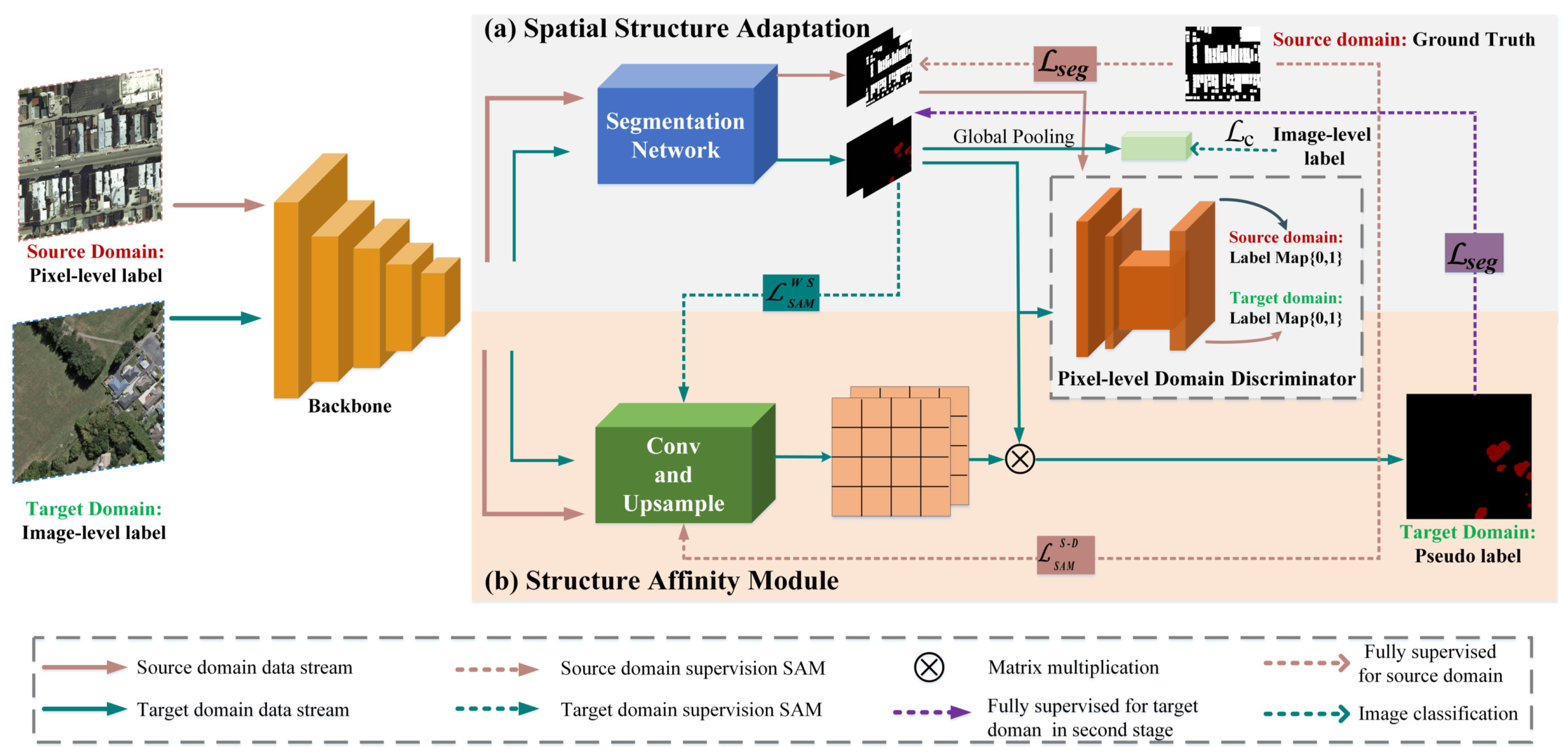
Figure 2 illustrates the overall framework of the CDSA. Our weakly supervised building segmentation method is trained in two stages. In the first stage, CDSA is trained by a source domain with pixel-level annotated and an image-level labeled target domain. In the second stage, in addition to the aforementioned supervision information, the segmentation results predicted by the first stage are used as pixel-level pseudolabels to supervise the target domain (as shown by the purple dotted line in Figure 2). Both the first stage and second stage consist of SSA and SAM.
Specifically, as shown in Figure 2, the components of CDSA are mainly divided into the backbone, segmentation network, pixel-level domain discriminator and SAM. Among these, the segmentation network and pixel-level domain discriminator constitute the SSA. The backbone as a feature extractor is designed based on the most advanced CNNs. In this paper, we remove the last fully connected layer of DenseNet [32] and utilize the remaining convolutional layers to learn the multilevel structure information of the input images. For the first and second stages, we use FCN [16] and DeepLabV3 [33] as segmentation networks to learn multiscale semantic information respectively. To increase the computational efficiency, we resize the input image of the feature extractor to .
3.2. Spatial Structure Adaptation
In the cross-domain building segmentation task, the source domain images have pixel-level annotated ground truth while the target domain has only image-level annotations. Clearly, how to obtain the most information from the source domain to understand the spatial structure features of buildings is still an open problem. Unfortunately, due to the various imaging conditions and sensor parameters, the texture, color and other characteristics of the building are diverse in different domains. Recently, domain adaptation [34,35] has been applied to map domain-invariant structure features to the target domain by adversarial learning. This strategy effectively reduces the impact of domain shift. However, these existing methods are still limited because they do not adequately consider the inter-pixel structure relationships on the cross-domain images. Therefore, the cross-domain transmission of inter-pixel structure affinity needs to be further studied.
In this paper, the SSA is proposed to generate the initial predicted probability maps by a weakly supervised domain adaptation approach. Meanwhile, the structure affinity is infused into the target domain via an iterative update weight of SSA and SAM (introduced in Section 3.3). Specifically, the segmentation network first learns the discriminative structure features of buildings in the input images. To determine whether the object exists in target domain images, a classification loss is defined using the image-level labels so that the segmentation network can focus on the objects. Then, the pixel-level domain discriminator is designed to distinguish which domain the feature comes from and further utilizes adversarial learning to align the spatial structure distribution of two domains. Besides, the predicted probability maps obtained by SSA are exploited to optimize the SAM, a process that implicitly propagates structure affinity relationships from the source domain into the target domain.
3.2.1. Weakly Supervised Segmentation
In the pixel-level labeled source domain , we define the training data as , where is the n-th training image, and is the pixel-level ground truth. Each element of is 0 or 1, representing that the i-th pixel belongs to the background or building. Similarly, the training data of target domain are denoted as , in which is either 1 or 0, which is 1 if the training image contains the building; otherwise, it is 0. We apply the segmentation network to generate segmentation predictions on both domains, where are the spatial dimensions of the input image after passing through the segmentation network and C is composed of building and background probability maps. In the source domain, we optimize the segmentation network by the loss between the predicted results and ground truth, which is defined as follows [23]:
where indicates the predicted probability value that the i-th pixel is the building. In addition, image-level labels of the target domain are employed to predict whether the object exists in the training image so that the segmentation network can recognize it. In other words, we first input to extract the features and then utilize the segmentation network to obtain the corresponding . Finally, we input into a global average pooling layer to obtain the predicted values for the corresponding categories:
where represents the predicted probability that the c-th category appears in the image and is a sigmoid function. Therefore, we use the predicted probability value p and the image label to calculate the category-wise binary cross-entropy loss:
where p denotes the predicted probability of the building. We compute between the predicted values and the image-level labels and propagate it backward to make the segmentation network predict the correct semantic categories. For example, when the source model is used to predict images of the target domain, the segmentation network can correctly identify the categories in a particular target image. The above procedures are described in the gray box of Figure 2.
3.2.2. Pixel-Level Domain Adaptation
To decrease the domain shift from the source and target domains, we propose to apply the pixel-level domain discriminator (PDD) to perform spatial structure feature alignment. In particular, the PDD is composed of three convolutional layers and a deconvolutional layer, and a sigmoid function, as shown in the dotted box of Figure 2. Specifically, the PDD receives , from the segmentation network and outputs a 2D-channel score map, where each pixel value represents the confidence score of the domain category. The loss of the PDD is defined as follows [36]:
where and with size of are the output results of the PDD. Meanwhile, through the adversarial learning of the SSA, the segmentation network can learn domain-invariant spatial structure features. The loss is defined as [36]:
Finally, the optimized objectives are written as follows [36]:
where and are the parameters of the PDD and segmentation network, respectively. and are the hyperparameters that control the importance of optimization functions. In the training process, we follow the training strategy of the GAN [37] that alternately updates the weights of the segmentation network and pixel-level domain discriminator.
3.3. The Structure Affinity Module
Although the SSA can provide additional spatial structure distribution for the target domain, it is still difficult to extract the regular edges of buildings. To take advantage of context information from existing data, the affinity matrix is introduced to describe the relationship between the pixel pairs. The affinity matrix can implicitly convey context information that is beneficial for the refinement of object edges. Specifically, we design the SAM (as shown in the lower pink box of Figure 2) to learn the structure affinity between the pixels in the input images. Then, the predicted affinity score is converted into an affinity matrix, and the matrix is applied to optimize the predicted probability maps obtained by SSA. Hence, the process improves the quality of the segmentation results by refining the edges of buildings.
The architecture of the SAM is shown in Figure 3b. To learn the structure affinity relationships under different receptive fields, we first use convolution to reduce the dimensionality of the last three layers of the feature extractor. Next, due to the different sizes of the last three layers, we adopt upsampling to align the size of the feature maps and then concat them. Finally, we use convolution to obtain the affinity feature maps to calculate affinity scores. The structure affinity of the pixel pairs on the output feature map is calculated to obtain the affinity matrix M. The feature maps of different layers of the backbone contain structure information in multiple fields of view and contacting them can make the affinity of the calculation more accurate. In other words, for an affinity feature map , where are the spatial dimension of the image after affinity feature extraction and D is the number of channels, we calculate the relationship between each pixel pair, so that the affinity matrix M contains connections. Theoretically, it is better to calculate the affinity of all pixel pairs on . Because the object of remote sensing images is usually small, we only need to consider the context of a local region in practice. Hence, we calculate the structure affinity between the pixel pairs with a radius of r in this paper. Finally, the affinity score between pixels i and j is defined as [38]:
where is the norm and indicates the feature of the i-th pixel on the . By training SAM, we can calculate the structure affinity between the pixels in a given image. And SAM can further refine the object via the propagation of structure context relationships (introduced in Section 3.3.3).
However, when calculating the affinity of paired pixels by Equation (10), we need to provide supervised information for SAM. Under fully supervised conditions, ground truth can be used to provide accurate structure affinity labels for SAM so that an affinity matrix can perfectly convey the context relationship between the pixels. Nevertheless, as the target domain is only annotated at the image level, it cannot directly provide affinity labels for SAM training. For this purpose, the predicted probability map of the target domain obtained by SSA is introduced to provide pseudosupervised information for SAM in our method. However, contains some low-confidence regions that do not participate in supervised training. After training the SSA, the structure affinity is infused into the target domain. Therefore, we propose to further integrate the structure context information from the source domain for training SAM.
3.3.1. Affinity Learning of Weakly Supervised Pseudolabel
Different from the pixel-level ground truth, the structure information of is inaccurate and cannot be directly used as the basis of supervision. Therefore, when assigning labels, we need to ignore the regions with relatively low confidence in . That is, some regions in the predicted probability maps that cannot fully be confirmed as belonging to the foreground or background will not participate in the loss function calculation of SAM. To highlight the foreground and background regions, we assign different exponential powers to the background channel of , and the remaining part is the discarded area with low confidence. For a pair of pixels in a high-confidence area, as shown in Figure 3a, if the pixels belong to the same category, the affinity label is set to ; otherwise, . Therefore, except for the areas with low confidence that do not participate in the training, the pixel pair set Q formed within the radius r is divided into two parts: pixel pairs belonging to the same category and pixel pairs belonging to different categories. Specifically, Q can be defined as [38]:
is a set of pixel pairs belonging to the same category, and its subset is divided into a foreground pixel pair set and a background pixel pair set. On the other hand, is a set of pixel pairs belonging to different categories. Then, the loss of a subset of Q is described as [38]:
where denotes the number of elements. Finally, in the weakly supervised condition, the loss of training SAM to learn structure affinity is defined as [38]:
Thus the trained SAM decides the class consistency between two adjacent pixels. That is, for pixels at the edges of the object, foreground affinity scores are higher than background. To show a better understanding, we visualize the affinity learning results in the ablation experiments.
3.3.2. Mining Cross-Domain Affinity
When mining the structure affinity of the source domain, there is a significant difference in the acquisition of the affinity labels. This is mainly because the source domain contains real pixel-level annotations to provide accurate context information for the network, so that every pixel of the source domain participates in the loss calculation. Similar to learning structure affinity on the target domain, for the source images, the feature extractor extracts multi-level features and calculate the association relationship of the pixel pairs by Equation (10). We note that prior to calculating the loss, we need to downsample the ground truth to the size of (consistent with the size). The difference is that we can directly understand the relationship between pixel pairs from the ground truth that is described as:
According to Equations (11)–(13), the loss of structure affinity learning in the source domain, , is defined to be the same as the .
Based on the aforementioned description, we mine the cross-domain structure affinity of remote sensing buildings. On the one hand, meaningful affinity is learned of the target domain to fit the existing pseudolabel supervision. On the other hand, the learned affinity of the source domain provides more complementary information. The total loss of SAM is shown as Equation (15).
3.3.3. Affinity Spread
After training the CDSA, SSA infuses the structure affinity of the source domain into the target domain. Therefore, SAM can provide a more accurate affinity matrix for SSA. As shown in Figure 3b, the backbone extracts features of input images, and then the features flow to SSA and SAM to generate the predicted probability maps and affinity feature maps, respectively. Finally, the paired structure affinity calculated by Equation (10) is transformed into a matrix to spread affinity information on the predicted probability maps. This process is realized using a random walk strategy [39]. Specifically, this process of spreading information is shown in Figure 4, which is described by:
where ∘ is the Hadamard power of the affinity matrix and is the hyperparameter. The diagonal matrix E represents the row normalization of M. Structure affinity spread is achieved by multiplying the transition matrix K with . The optimized is given by:
where v refers to the number of iterations and vec(·) denotes the vectorisation of a matrix.
3.4. Training Design of CDSA
Since we learn the affinity information of pixel pairs on the feature map of size , the size of the final affinity matrix is . When using the affinity matrix to optimize the predicted probability maps, we need to ensure the size consistency, so the size of SSA output is . Due to the small receptive field, semantic information is inevitably lost. Therefore, to facilitate network learning of multiscale semantic information, we design a multiscale fusion training strategy. For the source domain images, the SSA can obtain predicted results of different sizes and then calculate the loss with ground truth, shown as in Figure 5.
Figure 6 illustrates the entire training procedure for the target data. In training phase, the SSA and SAM are simultaneously optimized to generate predicted probability maps and affinity matrices, respectively. On the one hand, the SSA can learn spatial structure domain-invariant features to generate better . On the other hand, the SSA can infuse the structure affinity into the target domain and the SAM can further provide a more accurate affinity matrix to refine . In this process, we obtain precise structure affinity by minimizing . Finally, the optimized segmentation results are used as the pixel-level pseudolabels for the second stage. The entire process of the CDSA network is briefly summarized in Algorithm 1.
| Algorithm 1 The pseudocode for CDSA. |
|
4. Experiments
In this section, we present the validity of our CDSA. We simply describe the data sets, evaluation metrics, and experimental setup. Then, ablation experiments are designed to evaluate the effects of the key component of the CDSA. Finally, we analyze quantitative comparison results with some exiting methods and present a series of qualitative results.
4.1. Data Sets
4.1.1. Inria
Inria [40] are data extracted from aerial image buildings, including aerial orthographic color images and corresponding binarized building outlines in the images. Its spatial resolution is 0.3 m. To facilitate training, we crop each image to a size of . We split the training set into 1–5 images (2500 images with px) used for testing and 6–36 images (15,500 images with px) used for training.
4.1.2. WHU
WHU [41] is collected from the New Zealand Land Information Service website, which is the aerial image data set with a ground resolution of 0.3 m. The ground truth contains two semantic categories: building and background. The area contains 22,000 individual buildings, which are split into 8189 images of size. We choose 4736, 1036, and 2417 images for training, validation, and testing.
4.1.3. ISPRS
ISPRS [42] is obtained from the International Society for Photogrammetry and Remote Sensing (ISPRS) Commission II/4. We divide the ground truth into two categories (including building and background) and crop the patches with a size of . From the Potsdam data set, we choose 10,960, 9864 images for training and testing. From the Vaihingen data set, we select 1253 images as the training set and 1184 images as the test set.
4.2. Evaluation Metrics
In this study, we evaluate the performance of the proposed method in terms of both quantitative and qualitative aspects respectively. In qualitative analysis, we compare the results by visualizing the segmentation maps. We select two comprehensive quantitative metrics for evaluating the quality of our CDSA including intersection over union (IoU) and overall accuracy (OA).
IoU calculates the ratio of intersection and union of the two sets of the true and predicted values. It is defined as:
where is the predicted value and is the ground truth.
OA is the ratio of pixels with correct marking and the total pixels. Concretely,
where TP, TN, FP and FN are the result of pixel segmentation, which represent the number of elements in the true positive, true negative, false positive, and false negative pixel sets, respectively.
4.3. Implementation Details
We use DenseNet-169 [32] pretrained on ImageNet [43] as the feature extractor of the proposed method because it can achieve the desired performance with fewer parameters than other architectures. Our network is based on the PyTorch framework and is trained on two NVIDIA GeForce RTX 2080 Ti GPUs. We employ the Adam optimizer [44] to train the network with a learning rate of 1 × and momentum of 0.9. During training, the preprocessing of the image randomly crops a block of 9/10 the original image size, resizes it to , and sets the batch size to 8. For training SSA, we fix to 1 and to 0.0001. To reduce the number of network calculations, we choose to learn the affinity of pixel pairs in the range of in the experiment. In addition, in Equations (14) and (15), we fix to 8 and v to 6. During testing, the input image is resized to . Finally, the predicted segmentation result is adjusted to the input image size with upsampling methods.
4.4. Ablation Studies
To better evaluate the effects of the CDSA, ablation experiments are designed to analyze the contributions of the key component on the WHU data set.
4.4.1. Influence of the Pixel-Level Domain Discriminator
We first reveal the contributions of the pixel-level domain discriminator by integrating it into the SSNet framework. The SSA reduces the difference in spatial structure distribution between the source and target domains by adversarial learning. As shown in Table 1, the performance in terms of IoU is increased from 55.03% to 56.17%, and OA is increased from 93.36% to 93.42%, proving that the participation of the pixel-level domain discriminator effectively improves the segmentation accuracy in the target domain.
4.4.2. Influence of SAM under Weakly Supervised Learning
As shown in Table 1, structure affinity learned under weak supervision can effectively improve segmentation performance by improving the IoU score from 55.03% to 56.64% and the OA score from 93.36% to 93.51%. The main reason is that SAM has the ability to learn the contexts of buildings with information based on the structure affinity of target domains. By using the learned structure affinity to refine objects, more accurate segmentation objects can be obtained.
4.4.3. Influence of SAM under Cross-Domain Supervised
Based on the structure affinity under weakly supervised learning, we further study the contribution of cross-domain supervision to SAM. As shown in Table 1, we not only add a pixel-level domain discriminator to reduce domain differences and simultaneously infuse structure affinity of the source domain into the target domain, but also mine cross-domain structure affinity to provide complete supervision for SAM. In addition, collaboration between the SAM under cross-domain supervision and SSA leads to further improvements, with IoU increasing by 1.23% and OA increasing by 0.33%. This shows that on the basis of spatial structure feature alignment, cross-domain mining of structure affinity helps to improve the segmentation performance.
To more clearly understanding the structure affinity of pixels, we analyze the visualization results for the affinity performance in Figure 7. It is observed from the Figure 7b that the same pixels in the interior of the building indicate that they belong to the same structure. The border between the foreground and the background is more highlighted, indicating that the two have a low affinity score. Therefore, structure affinity can show the relationship between the pixels well. We use this relationship to spread context structure information in a segmentation map to refine the sides and corners of rectangular buildings.
4.5. Comparisons with State of the Arts
Here, we compare with existing domain adaptation, weakly and fully supervised methods.
4.5.1. Comparison with Weakly Supervised
For the foreground building category, we first show our comparison results on the WHU data set. As shown in Table 2, compared with WILDCAT [45], SEAM [27], and ICD [46], our method achieves 33.09%, 32.39%, and 33.55% improvements in the IoU score, respectively. In addition, we also show the comparison results in terms of IoU and OA on the Vaihingen data set in Table 3. It is observed that CDSA is significantly better than the other weakly supervised methods. Due to the dense buildings and relatively similar targets and backgrounds in the remote sensing scene, CAMs can only highlight local targets in the image and possibly even the background. Only selecting CAMs to obtain pseudolabels for segmentation training will often introduce noise to network training. Baseline SSNet introduces existing pixel-level annotation data to achieve good performance. Due to the mining of structure affinity and the alignment of spatial structures, our CDSA can make great progress.
4.5.2. Compared with Domain Adaptation
Table 2 illustrates the comparison results of domain adaptation as measured with IoU and OA scores on the Inria-WHU data sets. NoAdapt indicates that the model trained in the source domain without any domain adaptation is applied directly for testing in the target domain. We can observe that CDSA significantly outperforms other methods in terms of IoU and OA values on Inria→WHU and WHU→Inria data sets. In addition, as shown in Table 3, our method also achieves significant improvements on the Postdam-Vaihingen data sets. The major reasons for this are as follows:
- SSA can map the spatial structure domain-invariant features to the target domain and use image-level labels of the target domain to roughly locate objects.
- SAM can mine the structure context between the pixels to refine the edges of buildings.
4.5.3. Comparison with Fully Supervised
An examination of the results presented in Table 2 and Table 3 shows that our method further narrows the gap with the fully supervised segmentation network. FCN [16] and DeepLabV3 [33] can achieve excellent segmentation performance that relies on manually annotated pixel-level labels. However, compared with fully supervised methods, we can obtain quite competitive results by mining the cross-domain structure affinity under weakly supervised conditions. Therefore, our proposed CDSA network is also promising.
4.6. Qualitative Results
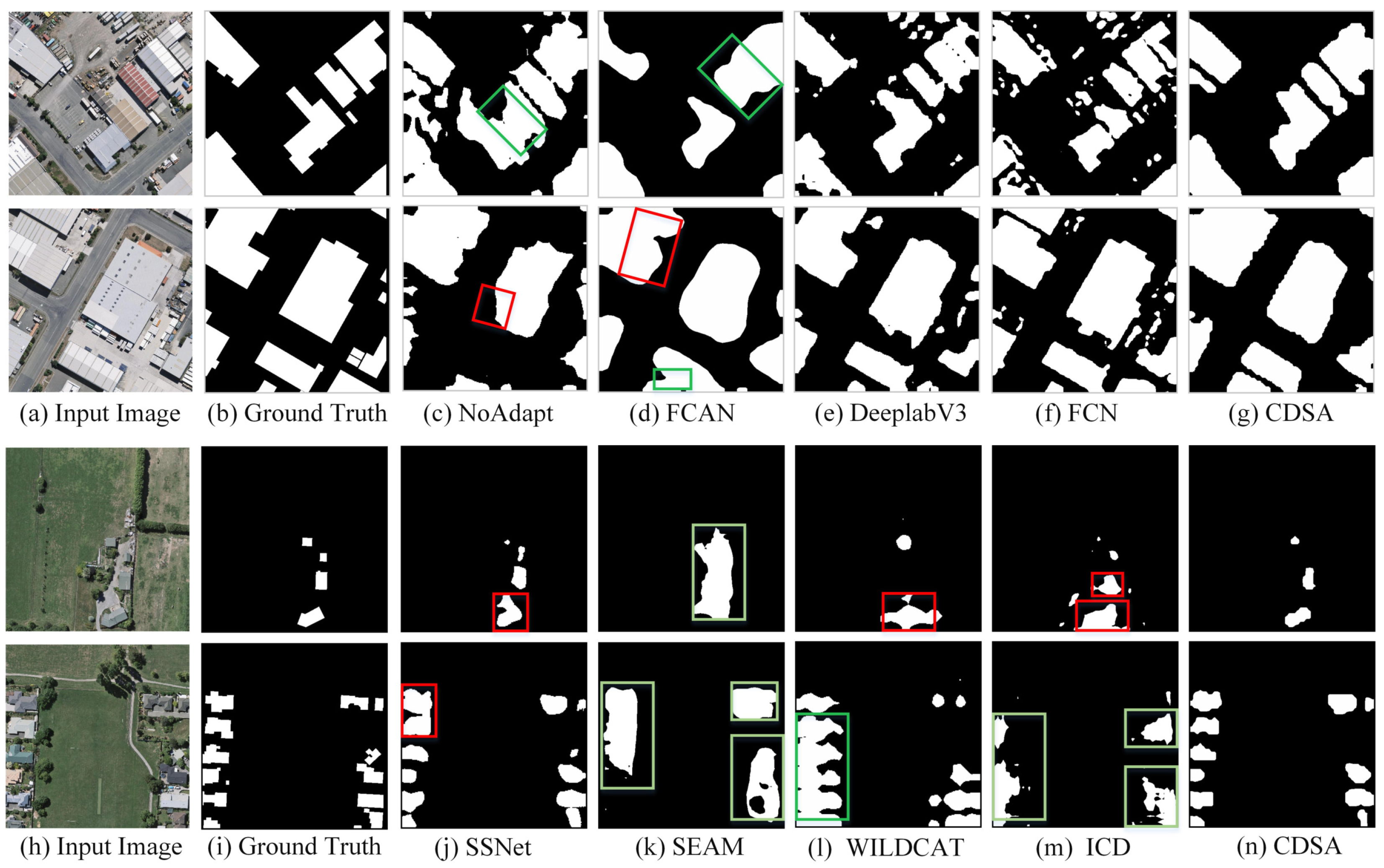
In Figure 8 and Figure 9, we further present the qualitative comparison results to confirm the effectiveness of our CDSA network on the WHU and Vaihingen data sets. In Figure 8, due to the low resolution of the data set, most of the objects in the remote sensing images are densely arranged and occupy a small image area. Methods that rely on a single dataset to obtain a localization map for segmentation (e.g., SEAM, ICD, WILDCAT) are only able to roughly localize the location of an object. However, the disadvantage of these methods is they do not accurately identify the narrow background between densely arranged dense buildings, resulting in buildings without clear boundaries (as shown Figure 8 green boxes). With the introduction of existing datasets to guide the segmentation task, SSNet, while improving in identifying narrow backgrounds, still has shortcomings for segmenting the edges of some buildings. Meanwhile, as shown in Figure 9 red boxes, some weakly supervised and domain adaptation methods still had the issue of irregular building boundaries. In brief, although CDSA is not accurate enough in predicting the borderlines compared to fully supervised networks, it obtains an advantage over other weakly supervised methods on the two data sets by refining the segmentation results. As shown in Figure 8, some failure segmentation results also are shown, i.e., CDSA cannot accurately locate small objects that are closely arranged in the image. We still need a new solution to address the aforementioned challenging.
5. Conclusions
When the remote sensing images are in low resolution and quality, obtaining refined labels are difficult. We propose a weakly supervised segmentation network based on mining cross-domain structure affinity, named CDSA, for refining buildings in remote sensing images. The proposed network mainly contains two branches, namely SSA and SAM. SSA adopts a domain adaptive approach to map domain-invariant spatial structure features to the target domain and also infuses structure affinity of source domain to the target domain. To improve the segmentation performance for regular structure buildings, SAM is designed to learn the structure affinity from the cross-domain and further optimize the building boundary. We analyze the architecture of CDSA in detail, and then conduct a large number of experiments at the two public data sets: Inria-WHU and Postdam-Vaihingen data sets. For detail, our method achieved IoU and OA scores of 57.87% and 93.84%, respectively, tested on the WHU data set. And CDSA can obtain IoU and OA scores of 79.57% and 94.52%, respectively, tested on the Vaihingen data set. The quantitative comparisons clearly indicate that CDSA performs better than other advanced methods in refining the edges of buildings. In the future, we will also conduct experiments on other types of remote sensing images to prove that the proposed network can be applied to a wider range of data sets.
Author Contributions
Investigation, J.Z., Y.L. and Z.S.; Methodology, J.Z., Y.L. and B.P.; Writing —original draft, Y.L.; validation, Y.L. and P.W.; Writing—review & editing, B.P., Z.S. and P.W. All authors have read and agreed to the published version of the manuscript.
Funding
This research was funded by the National Key R&D Program of China under the Grant 2019YFC1510905, the National Natural Science Foundation of China under the Grant 62001252 and 61902106, the Scientific and Technological Research Project of Hebei Province Universities and Colleges under Grant ZD2021311, the Natural Science Foundation of Tianjin under the Grant 19JCZDJC40000, and the Natural Science Foundation of Hebei province of China F2020202008.
Institutional Review Board Statement
Not applicable.
Informed Consent Statement
Not applicable.
Data Availability Statement
The datasets presented in this study are available public datasets.
Acknowledgments
The authors would like to thank the Group of Photogrammetry and Computer Vision (GPCV) of Wuhan University for providing the WHU data set, the International Society for Photogrammetry and Remote Sensing (ISPRS) Commission II/4 for providing the ISPRS data set, and the Inria data set provided by https://project.inria.fr/aerialimagelabeling/ (accessed date: 12 January 2022).
Conflicts of Interest
The authors declare no conflict of interest.
References
- Wang, Q.; Gao, J.; Li, X. Weakly supervised adversarial domain adaptation for semantic segmentation in urban scenes. IEEE Trans. Image Process. 2019, 28, 4376–4386. [Google Scholar] [CrossRef] [PubMed] [Green Version]
- Ren, P.; Xu, M.; Yu, Y.; Chen, F.; Jiang, X.; Yang, E. Energy minimization with one dot fuzzy initialization for marine oil spill segmentation. IEEE J. Ocean. Eng. 2018, 44, 1102–1115. [Google Scholar] [CrossRef] [Green Version]
- Milosavljević, A. Automated processing of remote sensing imagery using deep semantic segmentation: A building footprint extraction case. ISPRS Int. J. Geo-Inf. 2020, 9, 486. [Google Scholar] [CrossRef]
- Shi, Y.; Li, Q.; Zhu, X.X. Building segmentation through a gated graph convolutional neural network with deep structured feature embedding. ISPRS J. Photogramm. Remote Sens. 2020, 159, 184–197. [Google Scholar] [CrossRef]
- Wu, G.; Shao, X.; Guo, Z.; Chen, Q.; Yuan, W.; Shi, X.; Xu, Y.; Shibasaki, R. Automatic building segmentation of aerial imagery using multi-constraint fully convolutional networks. Remote Sens. 2018, 10, 407. [Google Scholar] [CrossRef] [Green Version]
- Zhu, Q.; Li, Z.; Zhang, Y.; Guan, Q. Building extraction from high spatial resolution remote sensing images via multiscale-aware and segmentation-prior conditional random fields. Remote Sens. 2020, 12, 3983. [Google Scholar] [CrossRef]
- Gupta, R.; Shah, M. Rescuenet: Joint building segmentation and damage assessment from satellite imagery. In Proceedings of the 2020 25th International Conference on Pattern Recognition (ICPR), Milan, Italy, 10–15 January 2021; IEEE: Piscataway, NJ, USA, 2021; pp. 4405–4411. [Google Scholar]
- Lu, Z.; Chen, D.; Xue, D. Survey of weakly supervised semantic segmentation methods. In Proceedings of the 2018 Chinese Control And Decision Conference (CCDC), Shenyang, China, 9–11 June 2018; IEEE: Piscataway, NJ, USA, 2018; pp. 1176–1180. [Google Scholar]
- Rafique, M.U.; Jacobs, N. Weakly Supervised Building Segmentation from Aerial Images. In Proceedings of the IGARSS 2019—2019 IEEE International Geoscience and Remote Sensing Symposium, Yokohama, Japan, 28 July–2 August 2019; IEEE: Piscataway, NJ, USA, 2019; pp. 3955–3958. [Google Scholar]
- Zhang, M.; Zhou, Y.; Zhao, J.; Man, Y.; Liu, B.; Yao, R. A survey of semi-and weakly supervised semantic segmentation of images. Artif. Intell. Rev. 2020, 53, 4259–4288. [Google Scholar] [CrossRef]
- Fu, K.; Lu, W.; Diao, W.; Yan, M.; Sun, H.; Zhang, Y.; Sun, X. WSF-NET: Weakly supervised feature-fusion network for binary segmentation in remote sensing image. Remote Sens. 2018, 10, 1970. [Google Scholar] [CrossRef] [Green Version]
- Chen, J.; He, F.; Zhang, Y.; Sun, G.; Deng, M. SPMF-Net: Weakly supervised building segmentation by combining superpixel pooling and multi-scale feature fusion. Remote Sens. 2020, 12, 1049. [Google Scholar] [CrossRef] [Green Version]
- Zeng, Y.; Zhuge, Y.; Lu, H.; Zhang, L. Joint learning of saliency detection and weakly supervised semantic segmentation. In Proceedings of the IEEE/CVF International Conference on Computer Vision, Seoul, Korea, 27 October–2 November 2019; pp. 7223–7233. [Google Scholar]
- Bruzzone, L.; Carlin, L. A multilevel context-based system for classification of very high spatial resolution images. IEEE Trans. Geosci. Remote Sens. 2006, 44, 2587–2600. [Google Scholar] [CrossRef] [Green Version]
- Tuia, D.; Persello, C.; Bruzzone, L. Domain adaptation for the classification of remote sensing data: An overview of recent advances. IEEE Geosci. Remote Sens. Mag. 2016, 4, 41–57. [Google Scholar] [CrossRef]
- Long, J.; Shelhamer, E.; Darrell, T. Fully convolutional networks for semantic segmentation. In Proceedings of the IEEE Conference on Computer Vision and Pattern Recognition, Boston, MA, USA, 7–12 June 2015; pp. 3431–3440. [Google Scholar]
- Mou, L.; Zhu, X.X. Rifcn: Recurrent network in fully convolutional network for semantic segmentation of high resolution remote sensing images. arXiv 2018, arXiv:1805.02091. [Google Scholar]
- Huang, J.; Zhang, X.; Xin, Q.; Sun, Y.; Zhang, P. Automatic building extraction from high-resolution aerial images and lidar data using gated residual refinement network. ISPRS J. Photogramm. Remote Sens. 2019, 151, 91–105. [Google Scholar] [CrossRef]
- Shao, Z.; Tang, P.; Wang, Z.; Saleem, N.; Yam, S.; Sommai, C. Brrnet: A fully convolutional neural network for automatic building extraction from high-resolution remote sensing images. Remote Sens. 2020, 12, 1050. [Google Scholar] [CrossRef] [Green Version]
- Xie, Y.; Zhu, J.; Cao, Y.; Feng, D.; Hu, M.; Li, W.; Zhang, Y.; Fu, L. Refined extraction of building outlines from high-resolution remote sensing imagery based on a multifeature convolutional neural network and morphological filtering. IEEE J. Sel. Top. Appl. Earth Obs. Remote Sens. 2020, 13, 1842–1855. [Google Scholar] [CrossRef]
- He, S.; Jiang, W. Boundary-assisted learning for building extraction from optical remote sensing imagery. Remote Sens. 2021, 13, 760. [Google Scholar] [CrossRef]
- Zhu, Y.; Liang, Z.; Yan, J.; Chen, G.; Wang, X. Ed-net: Automatic building extraction from high-resolution aerial images with boundary information. IEEE J. Sel. Top. Appl. Earth Obs. Remote Sens. 2021, 14, 4595–4606. [Google Scholar] [CrossRef]
- Jadon, S. A survey of loss functions for semantic segmentation. In Proceedings of the 2020 IEEE Conference on Computational Intelligence in Bioinformatics and Computational Biology (CIBCB), Via del Mar, Chile, 27–29 October 2020; IEEE: Piscataway, NJ, USA, 2020; pp. 1–7. [Google Scholar]
- Fan, R.; Hou, Q.; Cheng, M.M.; Yu, G.; Martin, R.R.; Hu, S.M. Associating inter-image salient instances for weakly supervised semantic segmentation. In Proceedings of the European Conference on Computer Vision (ECCV), Munich, Germany, 8–14 September 2018; pp. 367–383. [Google Scholar]
- Wang, X.; You, S.; Li, X.; Ma, H. Weakly-supervised semantic segmentation by iteratively mining common object features. In Proceedings of the IEEE Conference on Computer Vision and Pattern Recognition, Salt Lake City, UT, USA, 18–22 June 2018; pp. 1354–1362. [Google Scholar]
- Sun, G.; Wang, W.; Dai, J.; Van Gool, L. Mining cross-image semantics for weakly supervised semantic segmentation. In Proceedings of the European Conference on Computer Vision, Glasgow, UK, 23–28 August 2020; Springer: Berlin/Heidelberg, Germany, 2020; pp. 347–365. [Google Scholar]
- Wang, Y.; Zhang, J.; Kan, M.; Shan, S.; Chen, X. Self-supervised equivariant attention mechanism for weakly supervised semantic segmentation. In Proceedings of the IEEE/CVF Conference on Computer Vision and Pattern Recognition, Seattle, WA, USA, 14–19 June 2020; pp. 12275–12284. [Google Scholar]
- Wang, S.; Chen, W.; Xie, S.M.; Azzari, G.; Lobell, D.B. Weakly supervised deep learning for segmentation of remote sensing imagery. Remote Sens. 2020, 12, 207. [Google Scholar] [CrossRef] [Green Version]
- Ma, F.; Gao, F.; Sun, J.; Zhou, H.; Hussain, A. Weakly supervised segmentation of SAR imagery using superpixel and hierarchically adversarial CRF. Remote Sens. 2019, 11, 512. [Google Scholar] [CrossRef] [Green Version]
- Wu, S.; Du, C.; Chen, H.; Xu, Y.; Guo, N.; Jing, N. Road extraction from very high resolution images using weakly labeled OpenStreetMap centerline. ISPRS Int. J. Geo-Inf. 2019, 8, 478. [Google Scholar] [CrossRef] [Green Version]
- Zhang, L.; Ma, J.; Lv, X.; Chen, D. Hierarchical weakly supervised learning for residential area semantic segmentation in remote sensing images. IEEE Geosci. Remote Sens. Lett. 2019, 17, 117–121. [Google Scholar] [CrossRef]
- Huang, G.; Liu, Z.; Van Der Maaten, L.; Weinberger, K.Q. Densely connected convolutional networks. In Proceedings of the IEEE Conference on Computer Vision and Pattern Recognition, Honolulu, HI, USA, 21–26 July 2017; pp. 4700–4708. [Google Scholar]
- Chen, L.C.; Papandreou, G.; Kokkinos, I.; Murphy, K.; Yuille, A.L. Deeplab: Semantic image segmentation with deep convolutional nets, atrous convolution, and fully connected crfs. IEEE Trans. Pattern Anal. Mach. Intell. 2017, 40, 834–848. [Google Scholar] [CrossRef] [Green Version]
- Tsai, Y.H.; Hung, W.C.; Schulter, S.; Sohn, K.; Yang, M.H.; Chandraker, M. Learning to adapt structured output space for semantic segmentation. In Proceedings of the IEEE Conference on Computer Vision and Pattern Recognition, Salt Lake City, UT, USA, 18–23 June 2018; pp. 7472–7481. [Google Scholar]
- Deng, X.; Yang, H.L.; Makkar, N.; Lunga, D. Large scale unsupervised domain adaptation of segmentation networks with adversarial learning. In Proceedings of the IGARSS 2019—2019 IEEE International Geoscience and Remote Sensing Symposium, Yokohama, Japan, 28 July–2 August 2019; IEEE: Piscataway, NJ, USA, 2019; pp. 4955–4958. [Google Scholar]
- Pan, Z.; Yu, W.; Yi, X.; Khan, A.; Yuan, F.; Zheng, Y. Recent progress on generative adversarial networks (gans): A survey. IEEE Access 2019, 7, 36322–36333. [Google Scholar] [CrossRef]
- Goodfellow, I.; Pouget-Abadie, J.; Mirza, M.; Xu, B.; Warde-Farley, D.; Ozair, S.; Courville, A.; Bengio, Y. Generative adversarial nets. Adv. Neural Inf. Process. Syst. 2014, 27, 2672–2680. [Google Scholar]
- Ahn, J.; Kwak, S. Learning pixel-level semantic affinity with image-level supervision for weakly supervised semantic segmentation. In Proceedings of the IEEE Conference on Computer Vision and Pattern Recognition, Salt Lake City, UT, USA, 18–23 June 2018; pp. 4981–4990. [Google Scholar]
- Lovász, L. Random walks on graphs. In Combinatorics, Paul Erdos Is Eighty; Janos Bolyai Mathematical Society: Budapest, Hungary, 1993; Volume 2, p. 4. [Google Scholar]
- Maggiori, E.; Tarabalka, Y.; Charpiat, G.; Alliez, P. Can semantic labeling methods generalize to any city? The inria aerial image labeling benchmark. In Proceedings of the 2017 IEEE International Geoscience and Remote Sensing Symposium (IGARSS), Fort Worth, TX, USA, 23–28 July 2017; IEEE: Piscataway, NJ, USA, 2017; pp. 3226–3229. [Google Scholar]
- Ji, S.; Wei, S.; Lu, M. Fully convolutional networks for multisource building extraction from an open aerial and satellite imagery data set. IEEE Trans. Geosci. Remote Sens. 2018, 57, 574–586. [Google Scholar] [CrossRef]
- Gerke, M. Use of the Stair Vision Library within the ISPRS 2D Semantic Labeling Benchmark (Vaihingen). 2014. Available online: https://research.utwente.nl/en/publications/use-of-the-stair-vision-library-within-the-isprs-2d-semantic-labe (accessed on 20 January 2022).
- Deng, J.; Dong, W.; Socher, R.; Li, L.J.; Li, K.; Li, F.F. Imagenet: A large-scale hierarchical image database. In Proceedings of the 2009 IEEE Conference on Computer Vision and Pattern Recognition, Miami, FL, USA, 20–25 June 2009; IEEE: Piscataway, NJ, USA, 2009; pp. 248–255. [Google Scholar]
- Kingma, D.P.; Ba, J. Adam: A method for stochastic optimization. arXiv 2014, arXiv:1412.6980. [Google Scholar]
- Durand, T.; Mordan, T.; Thome, N.; Cord, M. Wildcat: Weakly supervised learning of deep convnets for image classification, pointwise localization and segmentation. In Proceedings of the IEEE Conference on Computer Vision and Pattern Recognition, Honolulu, HI, USA, 21–26 July 2017; pp. 642–651. [Google Scholar]
- Fan, J.; Zhang, Z.; Song, C.; Tan, T. Learning integral objects with intra-class discriminator for weakly-supervised semantic segmentation. In Proceedings of the IEEE/CVF Conference on Computer Vision and Pattern Recognition, Seattle, WA, USA, 14–19 June 2020; pp. 4283–4292. [Google Scholar]
- Zhang, Y.; Qiu, Z.; Yao, T.; Liu, D.; Mei, T. Fully convolutional adaptation networks for semantic segmentation. In Proceedings of the IEEE Conference on Computer Vision and Pattern Recognition, Salt Lake City, UT, USA, 18–22 June 2018; pp. 6810–6818. [Google Scholar]
Figure 1.
(a) A popular weakly supervised segmentation route is to train a classification network with single domain information, from which class activation maps are derived as pseudosupervision information for further supervising segmentation network training. (b) Our CDSA segmentation network mines cross-domain structure affinity as context for weakly annotated data to benefit pseudolabel inference and object refinement.

Figure 2.
Illustration of the CDSA architecture. To tackle the challenges of domain shifts and ambiguous boundaries in remote sensing building images, (a) SSA extracts domain-invariant features and simultaneously infuses the structure affinity of the source domain into the target domain by aligning the spatial structure feature distribution. (b) SAM learns the affinity matrix by mining structure affinity from the ground truth in the source domain and predicted results in the target domain. Then, the learned affinity matrix is applied to refine the initial predicted results obtained by SSA.

Figure 3.
(a) Pixel pairs sampled within a radius of r are used to supervise the SAM. The affinity label is set to 1 if the pixel pair is from the same class, otherwise, the label is set to 0. Regions with low confidence (white region) are not involved in supervision. (b) Overall architecture of the affinity learning and spreading process in SAM. ‘UP’ denotes the upsampling operation.

Figure 4.
The process of affinity spread.

Figure 5.
Our multi-scale fusion strategy. The segmentation loss is used to learn semantic information in different receptive fields on the source domain.
Figure 5.
Our multi-scale fusion strategy. The segmentation loss is used to learn semantic information in different receptive fields on the source domain.

Figure 6.
The overview training framework for target domain data.

Figure 7.
Performance visual analysis of structure affinity on WHU and Vaihingen data sets. Among them, the first two columns are the visual comparison results on the WHU data set, and the latter two columns are the visual comparison results on the Vaihingen data set. (a) Input the target domain images. (b) The visualization results for the affinity in a certain direction. Affinity presents a good performance in describing the class consistency between pixels. (c) Segmentation result of baseline, in which a decent object localization map is obtained but building edges are poorly segmented. (d) CDSA utilizes the structure affinity of pixels for refining the buildings. (e) Ground Truth.

Figure 8.
Comparison of qualitative analysis results on the WHU data set (Source domain: Inria data set).
Figure 8.
Comparison of qualitative analysis results on the WHU data set (Source domain: Inria data set).

Figure 9.
Qualitative analysis results on the ISPRS data set (Source domain: Postdam data set, Target domain: Vaihingen data set).
Figure 9.
Qualitative analysis results on the ISPRS data set (Source domain: Postdam data set, Target domain: Vaihingen data set).


Table 1.
A Ablation Experiments On WHU Data Set (%).
| SSA | Baseline | ✓ | ✓ | ✓ | ✓ | ✓ |
| Pixel-level Domain Discriminator | ✓ | ✓ | ✓ | |||
| SAM | Weakly Supervised | ✓ | ||||
| Cross-domain Supervised | ✓ | ✓ | ||||
| Image-level labels of target domain | ✓ | ✓ | ✓ | ✓ | ||
| The first stage | IoU | 51.75 | 52.93 | 54.26 | 55.03 | 56.51 |
| OA | 92.42 | 93.30 | 93.28 | 93.43 | 93.56 | |
| The second stage | IoU | 55.03 | 56.17 | 56.64 | 57.19 | 57.87 |
| OA | 93.36 | 93.42 | 93.51 | 93.67 | 93.84 | |
Table 2.
Performence Comparisons (IoU AND OA) among Different Methods on the WHU Data Set (%).
| Methods | Sourec Domain | Target Domain | IoU | OA | |
|---|---|---|---|---|---|
| Weakly supervised Methods | WILDCAT [45] | - | WHU | 24.78 | 82.64 |
| SEAM [27] | - | WHU | 25.48 | 69.23 | |
| ICD [46] | - | WHU | 24.32 | 48.89 | |
| SSNet [13] | Inria | WHU | 55.03 | 93.36 | |
| CDSA(Ours) | Inria | WHU | 57.87 | 93.84 | |
| Domain adaptation Methods | NoAdapt | Inria | WHU | 35.60 | 86.10 |
| FCAN [47] | Inria | WHU | 40.79 | 91.74 | |
| CDSA(Ours) | Inria | WHU | 57.87 | 93.84 | |
| NoAdapt | WHU | Inria | 27.84 | 81.34 | |
| FCAN [47] | WHU | Inria | 35.05 | 87.41 | |
| CDSA(Ours) | WHU | Inria | 39.82 | 91.23 | |
| Fully supervised Methods | FCN [16] | - | WHU | 73.29 | 96.52 |
| DeeplabV3 [33] | - | WHU | 75.89 | 96.86 |
Table 3.
Performence Comparisons (IoU AND OA) among Different Methods on the Vaihingen Data Set (%).
Table 3.
Performence Comparisons (IoU AND OA) among Different Methods on the Vaihingen Data Set (%).
| Methods | Source Domain | Target Domain | IoU | OA | |
|---|---|---|---|---|---|
| Weakly supervised Methods | WILDCAT [45] | - | Vaihingen | 44.92 | 78.08 |
| SEAM [27] | - | Vaihingen | 30.49 | 75.38 | |
| ICD [46] | - | Vaihingen | 39.48 | 69.10 | |
| SSNet [13] | Postdam | Vaihingen | 75.73 | 93.18 | |
| CDSA(Ours) | Postdam | Vaihingen | 79.57 | 94.52 | |
| Domain adaptation Methods | NoAdapt | Postdam | Vaihingen | 21.92 | 65.91 |
| FCAN [47] | Postdam | Vaihingen | 45.00 | 67.19 | |
| CDSA(Ours) | Postdam | Vaihingen | 79.57 | 94.52 | |
| NoAdapt | Vaihingen | Postdam | 28.75 | 67.39 | |
| FCAN [47] | Vaihingen | Postdam | 35.96 | 76.06 | |
| CDSA(Ours) | Vaihingen | Postdam | 69.94 | 90.58 | |
| Fully supervised Methods | FCN [16] | - | Vaihingen | 79.20 | 94.06 |
| DeeplabV3 [33] | - | Vaihingen | 80.31 | 94.57 |
Publisher’s Note: MDPI stays neutral with regard to jurisdictional claims in published maps and institutional affiliations. |
© 2022 by the authors. Licensee MDPI, Basel, Switzerland. This article is an open access article distributed under the terms and conditions of the Creative Commons Attribution (CC BY) license (https://creativecommons.org/licenses/by/4.0/).
Share and Cite
MDPI and ACS Style
Zhang, J.; Liu, Y.; Wu, P.; Shi, Z.; Pan, B. Mining Cross-Domain Structure Affinity for Refined Building Segmentation in Weakly Supervised Constraints. Remote Sens. 2022, 14, 1227. https://0-doi-org.brum.beds.ac.uk/10.3390/rs14051227
AMA Style
Zhang J, Liu Y, Wu P, Shi Z, Pan B. Mining Cross-Domain Structure Affinity for Refined Building Segmentation in Weakly Supervised Constraints. Remote Sensing. 2022; 14(5):1227. https://0-doi-org.brum.beds.ac.uk/10.3390/rs14051227
Chicago/Turabian StyleZhang, Jun, Yue Liu, Pengfei Wu, Zhenwei Shi, and Bin Pan. 2022. "Mining Cross-Domain Structure Affinity for Refined Building Segmentation in Weakly Supervised Constraints" Remote Sensing 14, no. 5: 1227. https://0-doi-org.brum.beds.ac.uk/10.3390/rs14051227
Note that from the first issue of 2016, this journal uses article numbers instead of page numbers. See further details here.