Article

Time-Lag Effect of Vegetation Response to Volumetric Soil Water Content: A Case Study of Guangdong Province, Southern China

1
State Key Laboratory of Organic Geochemistry, CAS Center for Excellence in Deep Earth Science, Guangzhou Institute of Geochemistry, Chinese Academy of Sciences, Guangzhou 510640, China
2
Key Lab of Urban Environment and Health, Fujian Key Laboratory of Watershed Ecology, Institute of Urban Environment, Chinese Academy of Sciences, Xiamen 361021, China
3
University of Chinese Academy of Sciences, Beijing 100049, China
4
Guangdong Research Institute of Water Resources and Hydropower, Guangzhou 510610, China
5
Guangdong Ecological Meteorology Center, Guangzhou 510640, China
*
Author to whom correspondence should be addressed.
Submission received: 3 January 2022 / Revised: 2 March 2022 / Accepted: 3 March 2022 / Published: 8 March 2022

Abstract

:
The content of soil water affects the physiological activities of vegetation, and the type of vegetation also affects the soil water balance. It is of great significance to study the response of vegetation to soil moisture change, which is helpful for understanding the vulnerability of vegetation for regional and environmental protections. The response of vegetation to soil moisture in Guangdong Province from mid-October 2015 to the end of March 2017 was studied by using cloudy region drought index (CRDI) as the drought index and volumetric soil water content (VSWC) as the soil moisture index to measure the level of water stress on vegetation. Taking the peak and valley positions of CRDI and VSWC as characteristic points, the lag time of vegetation to volumetric soil water content was obtained by judging the difference between the peak and valley positions of the two indexes. The results indicate that the response of vegetation to volumetric soil water content in Guangdong lagged 3.33 periods (9–35 days) on average. When VSWC is sufficient, there is no obvious difference in time-lag between different types of vegetation. However, when VSWC is relatively insufficient, grass shows the fastest response to the change of volumetric soil water content. Both longitude and soil moisture affect the lag time of vegetation. Under the same conditions, the higher the soil humidity is, the longer the lag time is, and the longer the delay time is with the greater longitude. CRDI can reflect the time-lag effect between vegetation and VSWC in Guangdong, indicating it is a sensitive and applicable index for characterizing the time-lag phenomena of vegetation to soil moisture.

Graphical Abstract

1. Introduction

Climate conditions significantly affect vegetation growth in terrestrial ecosystems [1,2]. In general, vegetation growth primarily depends on climatic factors: temperature, precipitation, and radiation [3,4], and climate could explain approximately 54% of the variation in vegetation [5]. However, climate change sometimes does not show an immediate impact on vegetation, and the response of vegetation to climate change usually lags. In 1989, Davis first proposed the lag effect of vegetation on climate change (greenhouse warming) [6]. Subsequently, scholars have done a lot of related studies [7,8,9,10]. Wu et al. found that regarding the time-lag effects, the climatic factors explained 64% variation of the global vegetation growth, which was 11% relatively higher than the model-ignoring time-lag effects [1].
Soil water is one of the important indicators that reflects climate change, and also has a direct relationship with precipitation [11]. Soil water is the direct source of water consumption of vegetation, which directly affects the physiological activities of vegetation [12,13]. At the same time, soil moisture affects the dissolution and transfer of nutrients in the soil, the absorption of nutrients by vegetation, and the activities of soil microorganisms, which also play an important role in the growth of vegetation [14]. Therefore, soil moisture status not only determines the pattern of vegetation, but also determines the stability of vegetation, showing a great impact on the growth and distribution pattern of vegetation [15]. In addition, different vegetation types have different water balance relationships with soil, and soil moisture not only depends on soil characteristics, but also is closely related to vegetation types [16]. Vegetation affects soil moisture, and the change of soil moisture also has an important impact on the growth of vegetation [17,18]. However, the influence of soil moisture on vegetation also has a time-lag effect. Niu et al. analyzed the response of vegetation to soil moisture in Xijiang River Basin, southern China, and their results show that the time-lag effect of vegetation response is 0–96 days [19]. After the time-lag correlation, Zhang et al. found that vegetation growth showed an obvious time-lag effect on soil moisture change in the Loess Plateau [20]. Zhao et al. found that the time lag of drought on grass effect occurred within 2 to 3 months in Loess Plateau [8]. The research of the Western Amazon showed that the canopy structure and moisture of the forest decreased in response to the strong water deficit in 2005, it also continued to decrease when the precipitation recovered in the following years, and the decrease in canopy backscatter persisted until the next major drought, in 2010 [21]. Peng et al. investigated the cumulative and lagged effects of drought on vegetation during 1982–2015. They found lagged effect for 46.2% of the vegetated land area, and 2–6 lagged months for the lagged effect [22].
Most studies on the time-lag effect between vegetation and soil moisture are carried out in arid and semi-arid areas, because the vegetation in those areas is relatively simple and the growth mode is more obvious [8,20,21,22]. The time-lag effect of vegetation and soil moisture in Guangdong Province remains unclear with limited studies for the in situ area. This is because the climate and vegetation in Guangdong Province are more complex. Guangdong is located in the southern tip of the mainland of China. In terms of climate types, 71.6% of Guangdong is in the south subtropical zone, 20.8% in the middle subtropical zone, and 7.6% in the North tropical zone [23]. Due to the diversity of climate conditions, there are many kinds of vegetation and different growth patterns in Guangdong. There is no obvious seasonal change in vegetation index in Guangdong Province for either crops or natural vegetation, so the relevant research is difficult and limited.
CRDI has been proved to be able to reflect the drought situation of vegetation in Guangdong Province [24]. Therefore, this paper compares the time series indexes of CRDI and VSWC of different types of vegetation from October 2015 to March 2017, to obtain the time-lag effect of vegetation on soil moisture in Guangdong Province and the difference of lag-effect between different types of vegetation. This study can also be regarded as a study of vegetation vulnerability, which is of great significance to the study and assessment of regional drought risk.

2. Study Area and Data Preprocessing

2.1. Study Area

The study area, Guangdong, is located in the south of China, adjacent to the South China Sea [25]. It lies between 20°13′–25°31′N and 109°39′–117°19′E, belonging to the East Asian monsoon region. It is one of the most abundant areas of light, heat, and water resources in China [26]. The annual average temperature of Guangdong in 2016 was 22.3 °C (0.4 °C higher than usual), and the annual accumulated precipitation was 2321 mm (30% higher than usual) [27]. The spatial distribution of precipitation is affected by topography, showing a trend of more in the east and less in the west. The seasonal distribution of precipitation in 2016 is uneven, and the precipitation in January, March, April, August, and November is more than that in previous years, of which, the precipitation in January is 6.3 times higher than that in the same period of previous years. The precipitation in other months is similar to that in the previous year [27]. Guangdong is densely vegetated with nearly 90% of the province covered by various types of vegetation (Figure 1).

2.2. Data Source and Preprocessing

The basic data used to calculate the drought index comes from the Moderate Resolution Imaging Spectroradiometer (MODIS). MODIS data have a moderate resolution, long coverage time and a short revisit period and have great potential for large-scale drought monitoring [26]. The main data used in this paper are MODIS surface reflectance data (MOD09 and MYD09) with 250 m resolution in 8 days and cloud optical thickness data (MOD08 and MYD08) with 5 km resolution in 8 days. The cloud optical thickness data needed to be resampled to 250 m resolution by the nearest method before use.
The land use/land cover (LULC) data selected in this paper are the international geosphere biosphere program (IGBP) products from MODIS (MCD12Q1). The data is provided once a year with a resolution of 500 m. To facilitate the follow-up analysis, the 17 categories of IGBP were integrated into four categories. All types of woodland were classified as “forest”, all types of grassland were classified as “grass”, farmland and farmland and natural vegetation mosaic were classified as “agriculture”, and the permanent wetland, waterbody, bare land, ice, and snow were classified as “others”. In addition, the LULC data were resampled to 250 m resolution by the nearest method to unify the resolution of all remote sensing data.
The soil moisture station data were obtained from Guangdong Ecological Meteorology Center. There are 25 stations recording VSWC in Guangdong Province (Figure 1). The data were recorded every hour from the middle of October 2015 to the end of March 2017. The station data of VSWC were combined into 8-day data corresponding to remote sensing data by averaging. The average VSWC in 8 days was used as the measurement index of soil moisture. The value of the station can also represent the soil moisture status of the surrounding area to a certain extent. Each station can correspond to an area of 5 × 5 pixels centered on the current pixel of the station. According to the LULC, the vegetation type of each station can be determined. Among all the stations, there are 9 pure grass stations, 2 pure forest stations, 4 mixed forest and grass stations, 3 mixed agriculture and grass stations, and 4 mixed grass and others stations (Table 1). Two of the 25 stations have no vegetation pixels in their corresponding 5 × 5 pixels area, and these two stations were eliminated.
Accurate measurements of soil moisture are limited by the number of field stations, and measuring soil moisture at a single location does not necessarily represent the condition of an entire region due to the large spatial heterogeneity of soil moisture [28,29,30]. Therefore, considering the large-scale time lag effect of this study, remote sensing soil moisture products are also needed as an auxiliary. Data sets such as Soil Moisture Active Passive (SMAP), Soil Moisture and Ocean Salinity (SMOS), Advanced Microwave Scanning Radiometer for Earth Observing System (AMSR2), Climate Change Initiative (CCI) can provide soil moisture parameters. Data products such as Gravity Recovery and Climate Experiment (GLDAS), ECMWF Reanalysis version 5(ERA5), etc., from soil moisture models or reanalysis are also available. Meng et al. downscaled the remote sensing soil moisture data of China with MODIS temperature vegetation dryness index (TVDI) [31]. They used China’s national meteorological stations and China’s agrometeorological and ecological observation network data to validate the effectiveness of downscaled soil moisture data [31]. Therefore, the soil moisture data with a resolution of 0.005° released to the public by them were used in this study (12 periods in 2016).

3. Methodology

3.1. Drought Index

There are many remote sensing indices that can be used to monitor drought, such as Normalized Difference Vegetation Index (NDVI) [32,33,34], Temperature Condition Index (TCI) [35], Crop Water Stress Index (CWSI) [36,37], Vegetation Health Index (VHI) [38,39], Temperature Vegetation Dryness Index (TVDI) [40,41], Vegetation Conditions Index (VCI) [42,43,44]. Due to the influence of cloud, the traditional remote sensing drought index data are usually missing, especially in cloudy regions like Guangdong. The annual total cloud cover of Guangdong is between 60% and 80% [45]. The cloud cover in spring and summer is relatively high, while the cloud cover in autumn is relatively low [46]. Cloud region drought index (CRDI) is a remote sensing drought index based on the inevitable relationship between cloud and precipitation and the continuity of drought. The main advantage of CRDI is that it can solve the problem of large area blank of drought data caused by cloud blocking in traditional remote sensing models, which has been well applied in Guangdong [24]. CRDI can be calculated by the following equations [24]:
CRDI = {   VCI ,   cloudless   region DI ( COT ,   ADI ) ,   cloudy   region
The basic remote sensing drought index VCI is still used in cloudless pixels. For the cloudy pixels which are unable to obtain drought data, the estimated drought value was used [24]. Among them, the COT (Cloud Optical Thickness) comes from MODIS, and the ADI (early drought index) is the CRDI of the previous period. CRDI ranges from 0 to 100. The larger the CRDI is, the better the vegetation condition is, indicating that drought will not occur in this area. The smaller the CRDI is, the worse the vegetation condition is, indicating that drought is more likely to occur in this area. This is similar to other remote sensing drought indices.

3.2. Smoothing Method

In the field of remote sensing, it is usually necessary to reconstruct the curve of time series. This is because some noise in remote sensing images will make the data fluctuate which cannot be ignored [47]. The reconstruction of the data can remove the noise in the curve and make the curve smoother. When comparing the trend of multiple curves, the trend of the reconstructed curve is more obvious and the contrast is stronger. The curve reconstruction method selected in this paper is WS (Whittaker smooth). WS was first introduced into the research of remote sensing image reconstruction by Eilers P.H. in 2003 [48]. It smoothes time series index by balancing fidelity and roughness [49,50]. WS has the advantages of fast and convenient, simple and controllable parameters and easy implementation [51,52]. It has been widely used in the analysis of time series curves in the field of remote sensing.

3.3. Framework for the Time-Lag Effect of Vegetation on VSWC

The time-lag effect of vegetation response to soil moisture of Guangdong was analyzed by comparing the positions of the peak and valley of similar sections of VSWC index and drought index. First, the data of VSWC were synthesized. Then, CRDI was calculated using MODIS data. Next, the time series data of VSWC and CRDI were smoothed and compared, and the time-lag was judged by comparing the location of peak and valley in similar section. The time-lag effect of vegetation response to soil moisture was analyzed by comparing the difference of peak and valley position of the two indexes. Based on the analysis of the time-lag effect of CRDI and soil moisture in different areas and different vegetation types, the spatial distribution of time-lag was obtained by regression method with Meng’s downscaled soil moisture data according to the value of corresponding peak and valley lag (Figure 2). For each pixel of MOD09/MYD09, a value is selected from all the acquisitions within the 8-day composite period. Therefore, when the difference between peak or valley values is n, the time-lag between peak or valley values fluctuated from (n − 1) × 8 + 1 days to (n + 1) × 8 − 1 days.

4. Results

4.1. Spatial Distribution of Soil Moisture

The downscale soil moisture data made by Meng [31] in 2016 are averaged to obtain the spatial distribution of soil moisture. The average soil moisture in Guangdong Province of 2016 was 0.347, which was above the national average. It can be seen from the spatial distribution of average soil moisture that the moisture in coastal areas is significantly higher and that in mountainous areas in northern Guangdong is slightly lower (Figure 3). In addition, the soil moisture at the junction of Guangzhou, Foshan, and Zhongshan where station 8 and station 10 are located is also low. This area is located in the coastal area, but the degree of urbanization here is high, so the vegetation coverage is relatively poor. Low vegetation coverage leads to the decline of soil water-holding capacity and lower soil moisture.

4.2. Time-Lag Effect of the Whole Province

The time series of VSWC and CRDI are constituted from the average value of each period. The two indexes started from the 38th period of 2015 and ended in the 20th period of 2017 (Figure 4a). During 2016, the highest CRDI value of the whole province was 86, and the lowest CRDI value was 57. The VSWC index fluctuated between 28 g and 34 g. The VSWC and CRDI are not consistent with each other, whether it is the position of peak and valley or their range of change. However, after moving the VSWC data backward for 3 cycles, it can be found that although there are still some differences in the variation range, the trend and the position of the peak and valley of these two indexes show a good correspondence (Figure 4b). It is the time-lag effect that causes the position of peak and valley of CRDI index to appear later than that of the VSWC index. Therefore, it can be determined that there is an obvious time-lag between vegetation and VSWC in Guangdong.
The peak and valley of CRDI and VSWC indexes need to be matched. Only segments with similar trend were selected for matching, and each peak/valley can be matched only once. When the difference between the position of the peak/valley on the CRDI index and the adjacent VSWC index is too small, this pair of peaks/valleys are not considered effective. Compared with the position of peak and valley of VSWC index, the position of peak and valley of CRDI index in Guangdong lagged longest by 5 periods and shortest by 1 period. The average time lag of the peak and valley of the two data is 3.33 periods. In general, the vegetation will show corresponding changes only after 19–35 days of soil moisture change in Guangdong Province (Table 2). In addition, the time-lag of the peak is longer than that of the valley.

4.3. Time-Lag Effect of Different Vegetation

Taking station 1 (the 5 × 5 pixels of which include forest and grass) and station 2 (the 5 × 5 pixels of which include agriculture and grass) as examples, the difference of the time-lag effect of different vegetation types at the same location was discussed. If the CRDI is slightly delayed, the trend between CRDI (after taking the average value of 5 × 5 pixels) and the VSWC index of these two stations have some similarities, especially in the second half of 2016, which is from 24th to 46th periods in 2016 (Figure 5).
The effective peak of station 1 was 4 pairs, which was lagged by 2, 4, 2, and 2 periods respectively. The average time lag was 2.5 periods (12~28 days). The effective valley of station 1 was 3 pairs, which is lagged 3, 2, and 2 periods respectively. The average time lag was 2.33 periods (11~27 days). The effective peak of station 2 was 4 pairs, which was lagged by 3, 4, 0, and 2 periods respectively. The average time lag was 2.25 periods (10~26 days). The effective valley of station 2 was 3 pairs, which was lagged 2, 1, and 3 periods respectively. The average time lag was 2 periods (8~24 days). No matter peak or valley, the lag time of station 2 is shorter than that of station 1. However, the two stations cannot be compared with each other due to the different proportions of the surrounding vegetation types. But the time-lag effect of different vegetation types at the same station can be compared.
The pixels of different vegetation types in the 5 × 5 pixels where station 1 and 2 is located were extracted and averaged respectively to obtain the CRDI indexes of different vegetation types at station 1 and 2. Within 5 × 5 pixels of the same station, the trend of different vegetation is the same, and the location of individual peak and valley is slightly different (Figure 6).
In the first half of 2016, the peaks and valleys of different vegetation types of the same station corresponded well, and there was no obvious time-lag. However, in the second half of 2016, the peaks and valleys of forest from station 1 and agriculture from station 2 were significantly more backward than the grass of those two stations. This indicates that the grass is more sensitive than forest and agriculture to the change of VSWC under the same soil moisture condition in the second half of 2016.
In order to further confirm whether the time-lag effect is related to vegetation type, it is necessary to distinguish the data of the first half and the second half of the year, and to calculate the correlation of different lag time between CRDI and VSWC indexes. The time series curves of stations 1 and 2 are divided into two sections, one is the first half of 2016 (1–23 periods), and the other is the second half of 2016 (24–46 periods). The correlations between CRDI of grass and forest (Figure 7a), grass and agriculture (Figure 7b) under different time lags were calculated.
The overall correlation coefficient of CRDI indexes of forest and grass in 2016 was 0.93. In the first half of 2016, the correlation between forest and grass was highest when the lag period was 0, and there was no obvious time lag between forest and grass (Figure 7). In the second half of 2016, the correlation between forest and grass was highest when the lag period was 1 (Figure 7a), and the forest lagged behind the grass for 1 period (1–16 days).
The overall correlation coefficient of CRDI indexes of agriculture and grass in 2016 was 0.86. In the first half of 2016, the correlation between agriculture and grass was highest when the lag period was 0, and there was no obvious time lag between agriculture and grass (Figure 7). In the second half of 2016, the correlation between agriculture and grass was highest when the lag period was 1 (Figure 7b), and the agriculture lagged behind the grass for 1 period (1~16 days).
The indexes of the two stations show that there is no obvious time lag between different types of vegetation in the first half of the year. In the second half of the year, forest and agriculture lagged behind grass for 1 period. Compared with the second half of the year, the VSWC in the first half of the year was higher, and there was no frequent drastic change. Under the condition of sufficient water, vegetation can grow normally according to its own growth pattern. In the second half of the year, VSWC was lower and fluctuated frequently. In this case, vegetation changes not only according to its own growth pattern, but also changes with the change of soil moisture. The grass had the fastest response to the change of VSWC, followed by agriculture and forest. This is because among the three vegetation types, grass has the shallowest root system. Precipitation and artificial irrigation are most likely to cause the change of VSWC. When water contacts the ground, it will slowly penetrate from the surface to the bottom, which takes a certain amount of time. In addition, it will be absorbed or lost in the process of infiltration. The shallower the root system is, the faster and more sufficient the time for the vegetation to absorb this kind of water is, so the faster the response to the change of soil moisture is. Therefore, the grass with a shallow root system had the fastest response to the change of soil moisture.

4.4. Time-Lag Effect of Different Geographical Locations

In order to discuss the difference in time-lag effect of vegetation in different geographical locations, the average CRDI of the same type of vegetation from 5 × 5 pixels of different stations were extracted. Then the indexes of CRDI and VSWC in different stations were compared. When selecting a station, if the target vegetation type is less than 20% (5 pixels) of the 5 × 5 pixels corresponding to the current station, the station will not be selected. In addition, if the change range of VSWC at the current station is too small, the VSWC is relatively stable, and there is no obvious increase or decrease. That indicates that there may be no effective peak or valley point between CRDI and VSWC indexes at this station, and the station will not be selected either.

4.4.1. Time-Lag Effect of Agriculture

Taking station 2 and station 3 as examples, the time-lag effect of CRDI on VSWC in the agricultural area was discussed. Station 2 is located in the Leizhou Peninsula, and station 3 is located in the eastern coastal area and has higher latitude (Figure 1). The indexes of CRDI of the two stations are similar. The planting patterns in these two areas may be similar. The indexes of VSWC in the two stations are similar, although the VSWC of station 2 was significantly higher than that of station 3. Only the peaks and valleys with the same location of the two stations are retained for comparison (Figure 8).
The two stations have three pairs of matched peaks and two pairs of matched valleys. The peak and valley of CRDI at station 2 lag behind the VSWC for 2 and 3 periods on average. The peak and valley of CRDI at station 3 lag behind the VSWC for 3 and 3 periods on average (Table 3). In contrast, the peak lag of station 2 is one more period (8 days) than that of station 3, and the valley lag has no significant difference. The latitude of station 2 is lower than that of station 3, and the average VSWC of station 2 is higher than that of station 3.

4.4.2. Time-Lag Effect of Forest

Among the VSWC stations in Guangdong Province, there are six stations containing forest type (within 5 × 5 pixels of the station). The selected stations 1, 4, and 5 contain forest and grass, and the selected station 6 is pure forest (Table 1). Station 1 and 4 are located in northern Guangdong, station 6 is located in eastern Guangdong, and station 5 is located in central Guangdong (Figure 1). Compared with the agricultural stations, the CRDI index of the four forest stations are not so similar. This is because there are great differences among forest types. Similar to agricultural stations, the same peak and valley for different stations cannot be chosen. Therefore, for the forest stations, it is possible to compare the corresponding situation of peak and valley of the corresponding sections with the same trend of CRDI and VSWC indexes (Figure 9).
The matched peaks of CRDI index in stations 4, 1, 5, and 6 lagged behind that of VSWC by 2.5, 3, 3.3, and 4.5 periods on average, respectively. The matched valleys of CRDI index in stations 4, 1, 5, and 6 lagged behind that of VSWC by 2, 2.5, 2.5, and 4 periods on average, respectively (Table 4). In contrast, the lag time of both peak and valley of station 4, 1, 5, and 6 increases in turn. The latitudes of stations 4, 1, 5, and 6 decreased in turn, while the VSWC increased.

4.4.3. Time-Lag Effect of Grass

Among the volumetric soil water content stations in Guangdong Province, there are twenty-one stations containing grass type (within 5 × 5 pixels of the station). The selected stations 4 and 7 contain forest and grass, stations 8 and 10 contain grass and other types, and the selected stations 5 and 9 are pure grass (Table 1). Station 5 and 7 are located in northern Guangdong, station 20 is located in eastern Guangdong, and station 11 is located in central Guangdong (Figure 1). The CRDI indexes of the grass stations are also not so similar. Therefore, for the grass stations, it is possible to compare the corresponding situation of peak and valley of the corresponding sections with the same trend of CRDI and VSWC indexes (Figure 10).
The matched peaks of CRDI index in stations 4, 5, 10, 8, 7, and 9 lagged behind that of volumetric soil water content by 2, 2.5, 2.5, 3, 3, and 4 on average, respectively. The matched valleys of CRDI index in station 4, 5, 10, 8, 7, and 9 lagged behind that of volumetric soil water content by 1.5, 1.7, 2, 2, 3, and 3.5 on average, respectively (Table 5). The latitudes and the average volumetric soil water content of stations 5, 8, and 9 are roughly the same, but the longitude increases in turn, and the lag time also increases in turn. The geographic location of stations 10 and 8 are very close, and the longitude and latitude are also very similar, but the volumetric soil water content of station 8 is higher than that of station 10, and the lag time of station 8 is also greater than that of station 10.

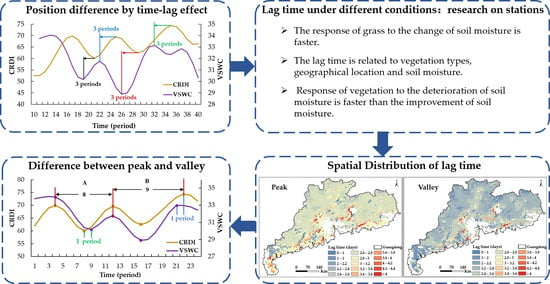
4.5. Spatial Distribution of Time-Lag

To further analyze the spatial distribution of the time-lag effect of CRDI on VSWC in Guangdong, we obtained the spatial distribution of the time-lag effect by regression method. First, the CRDI of different vegetation types in each station was extracted, and the corresponding peaks and valleys between VSWC and CRDI were matched in turn. Then, the average time-lag of peaks and valleys of different vegetation types at each station was calculated. Finally, the remote sensing data of soil moisture were introduced to establish the regression model between soil moisture and time lag of different vegetation types to obtain the spatial distribution of time lag in Guangdong Province. In this process, it is necessary to remove the stations with little change of VSWC and that has no obvious peak and valley of soil moisture in the whole year, and 21 stations were retained. There were 2 agricultural stations, 5 forest stations, and 14 grass stations reserved.
In general, the lag time of peak and valley is similar in spatial distribution, and the lag time of the peak is slightly longer than that of the valley. In the previous section, we concluded that the higher the VSWC, the longer the lag time maybe. In areas with high soil moisture, vegetation can grow according to its own growth pattern under the condition of sufficient water, and store a certain amount of water. When the VSWC in these areas decreases, the vegetation will first consume the stored water, and the response time of vegetation to the decrease of VSWC is slightly longer. When the VSWC in these areas rises, the response time to the rise of VSWC is also slightly longer because the vegetation itself is not short of water. In areas with low soil moisture content, the water reserves of vegetation are low and more dependent on the external water supply. Therefore, the vegetation in these areas is more sensitive to the change of external humidity.

5. Discussion

5.1. The Difference of Time-Lag between Peak and Valley

Compared with VSWC data, CRDI in Guangdong Province has obvious differences in the location of peak and valley. The time-lag of different vegetation types is different in different geographical locations. However, except for the agricultural stations, the lag time of the peak of most stations was significantly longer than that of the valley (Table 4 and Table 5 and Figure 11). If a complete process is defined, which includes two parts of decline and rise, it includes 2 peaks and 1 valley. To clarify this phenomenon, a forest station and a grass station were selected. Then the corresponding process of CRDI and VSWC were extracted, moving CRDI backward for comparison. It can be seen that the lag time of peak and valley in a certain period at the same station is also different (Figure 12).
Figure 12 shows three different situations of the response of CRDI to the change in VSWC. The VSWC at station 4 took 9 periods to complete the whole process, while CRDI took 8 periods. This is because the CRDI from the peak to the valley takes one period less than VSWC (Figure 12a). Both of them took 5 periods from the valley to the peak. Station 9 has two complete processes, A and B. The VSWC and CRDI at process A both took 8 periods to complete this process. CRDI is one period less than VSWC from the peak to the valley, and one period more from the valley to the peak. The VSWC at process B took 10 periods to complete this process, while CRDI took 9 periods. This is because the CRDI from the valley to the peak is one period more than VSWC (Figure 12a). Both of them took 4 periods from the peak to the valley. Although there are three different situations, they all show the same conclusion: compared with VSWC, CRDI takes a shorter time from the peak to the valley and a longer time from the valley to the peak. This shows that when the VSWC increases, the CRDI increases at a slower speed, and the response of vegetation to the increase of VSWC is slower. When the VSWC decreases, the CRDI decreases at a faster speed, and the response of vegetation to the decline of VSWC is also faster. Vegetation is more sensitive to water deficit.
However, there is no such pattern in agriculture stations. This is because the vegetation in agricultural areas is artificial vegetation, which involves artificial irrigation. Unless there is a serious drought, the drought situation in agricultural areas will be much better than that of natural vegetation. The growth pattern of vegetation in agricultural areas is usually affected by irrigation in the corresponding period.

5.2. Compared to Other Researchers

Niu et al. analyzed the time-lag between vegetation index and soil moisture content in Xijiang River Basin. This research shows that the time-lag in some areas of western Guangdong is 16–32 days, which is similar to that of the current study. But Niu et al.’s results show that the lag time near the Pearl River Delta reaches 60–80 days, which has a certain gap with the result of this study. However, they did not exclude the non-vegetation areas in their research, and the Pearl River Delta is a large area of the urban land gathering area, so there may be some deviation.
Different from choosing vegetation drought index and soil moisture data when studying the time-lag effect, many scholars chose vegetation index or precipitation in similar studies. Zhao et al. found that the lag time of drought on grass effect occurred within 2–3 months in the Chinese Loess Plateau [8]. This is a little longer compared with the result of this study. In addition to the different dry and wet conditions in the study area, on the one hand, vegetation may be more sensitive to soil moisture with the decline of latitude [14]. On the other hand, it may be that they used precipitation data. In fact, precipitation is the main reason for the change of soil moisture. The relationship between vegetation drought, soil moisture, and precipitation should be progressive, that is, soil moisture has a certain time-lag for precipitation, and drought has a certain time-lag for soil moisture.
It is found by Zhao et al. (2020) that the time-lag is longer in the years with low average precipitation, which is contrary to the conclusion of this study [8]. This may be because the Chinese Loess Plateau is a serious drought area, and the vegetation types and growth conditions are different from those of Guangdong Province. Or it can be inferred that when the water content is in a certain appropriate range, the lag of drought to water content is normal. The soil moisture condition of the Chinese Loess Plateau is lower than that of the general area. The lower the soil moisture is, the farther away it is from the comfortable value of vegetation and the more lag it has. The soil moisture condition in Guangdong Province is higher than that in other areas. The higher the soil moisture is, the farther away it is from the comfortable value of vegetation. When the water content is beyond the appropriate range, whether it is too low or too high, the response time of vegetation drought on VSWC will lag longer. Further research is needed to verify this conjecture.

5.3. The Improvement of this Research

Based on the difference of peak and valley position between CRDI and volumetric soil water content data, the time-lag of vegetation drought on soil moisture was studied. Through the discussion of the results, future research can be improved from the following aspects:
  • The accuracy of the data could be improved. The spatial resolution of remote sensing data is 250 m, and the resolution of land use/land cover data is 500 m. In addition, the temporal resolution of CRDI index is 8 days, and the interval between the two periods of data is 16 days at most and 1 day at least due to the rule of MODIS data processing. To further improve the accuracy, higher temporal and spatial resolution data can be considered.
  • The difference of section from peak to valley between the two data may be more contrastive. In this paper, the method of extracting the position of the peak and the valley was used to judge the time-lag. In fact, when determining the peak and the valley, the trend before and after the peak or the valley should be considered. But if the section from the peak to the valley or the valley to the peak can be quantified as a feature, it may help us make a better comparison.
  • Due to the existence of noise and other high-frequency components, the time difference between peak and valley in CRDI and VSWC sequences may be misleading and inaccurate. In other words, interannual and seasonal changes of time series are not considered in this paper, which is also one of the limitations of this paper. Wavelet analysis is a common method in time series analysis [53]. If the sequence can be further transformed, the time delay can be calculated more strictly in the time domain (representing the time difference between peak and valley) and scale domain (determining the effective peak and valley process). Cross wavelet has been proved to be an effective method to study the relationship between two-time series in time-frequency domain from multiple time scales [54,55,56]. Wavelet coherence and phase difference can identify the lead-lag nexus between two time series [57]. Besides, other wavelet transform methods can also be considered to be applied in the scenario of this paper. The wavelet analysis method will provide great help in the follow-up research.
In addition, the time-lag and cumulative effect of precipitation on vegetation can also be considered.

6. Conclusions

The response of vegetation to some external environmental changes has a certain time-lag effect. Studying the time-lag effect of vegetation response on VSWC is helpful for understanding the impact of climate change on vegetation in a specific area. Taking CRDI as the measure of vegetation drought and VSWC as the measure of soil moisture, it is found that the vegetation in Guangdong Province has time-lag effect on the change of VSWC. CRDI can reflect this phenomenon clearly. The time-lag effect of vegetation response on VSWC in Guangdong Province was analyzed, and the main conclusions are as follows:
  • The response of CRDI on VSWC in Guangdong lagged 3.33 periods (9–35 days) on average.
  • In the first half of 2016 when soil moisture was sufficient, there was no significant difference in time-lag between different types of vegetation in the same place. In the second half of 2016 when soil moisture was relatively deficient, the grass had the fastest response to soil moisture change due to its shallow roots, followed by forest and agriculture. But the grass is only one period faster (1–16 days)
  • The time-lag of stations with different geographical locations and VSWC was different. If latitude and VSWC are similar, the time-lag is longer when longitude increases; when longitude and latitude are similar, the time-lag is longer when VSWC is higher.
  • In natural vegetation, the lag time of the peak is usually longer than that of the valley. When VSWC decreases, the vegetation drought index will decline rapidly; when VSWC increases, vegetation drought index will rise at a slightly slower speed. This indicates that the response of vegetation to the deterioration of soil moisture is faster, and the response to the improvement of soil moisture is slightly slower.
Due to the inherent growth pattern of vegetation, if it does not break through a certain limit of soil moisture and last for a certain period, soil moisture can only affect the vegetation based on its inherent growth pattern. During vegetation growth, once VSWC decreases, even if it does not reach the severity of drought, vegetation growth will be affected to some extent. In other words, in the tropical and subtropical areas with high soil moisture, the growth status of vegetation is affected by the continuous change of soil moisture, and vegetation is still vulnerable to a certain extent. In addition, under the same climatic conditions, grass has the fastest response to the change of soil moisture, followed by agriculture and forest. It is better to irrigate the agriculture according to the moisture of soil and the growth of surrounding grass or shrubs before the crops show drought symptoms.

Author Contributions

W.L. proposed the research idea. W.L. and Y.W. determined the specific research methods. J.Y. and Y.D. processed the volumetric soil water content data. W.L. carried out the data processing and analysis and wrote the manuscript. All authors have read and agreed to the published version of the manuscript.

Funding

This study was funded by The Natural Science Foundation of China (U1901215, 41401485) and the Natural Science Fund of Guangdong Province (2021A1515011375, 2021A1515012579).

Institutional Review Board Statement

Not applicable.

Informed Consent Statement

Not applicable.

Data Availability Statement

Not applicable.

Acknowledgments

We appreciate the financial support from NSFC. We are grateful for the support we got from NASA for offering free access to its MODIS data and Guangdong Ecological Meteorology Center for volumetric soil water content data. Three anonymous reviewers are also acknowledged for their constructive comments which greatly improved the manuscript. This is contribution No. IS-3142 from GIGCAS.

Conflicts of Interest

The authors declare no conflict of interest.

Abbreviations

Acronym Table
CRDIcloudy region drought index
VSWCvolumetric soil water content
MODISmoderate resolution imaging spectroradiometer
LULCland use/land cover
IGBPinternational geosphere biosphere program
NDVInormalized difference vegetation index
TCItemperature condition index
CWSIcrop water stress index
VHIvegetation health index
TVDItemperature vegetation dryness index
VCIvegetation conditions index
SMAPsoil moisture active passive
SMOSsoil moisture and ocean salinity
AMSR2advanced microwave scanning radiometer for Earth observing system
CCIClimate Change Initiative
GLDASgravity recovery and climate experiment
ERA5ECMWF reanalysis version 5
TVDItemperature vegetation dryness index
WSWhittaker smooth
COTcloud optical thickness
ADIantecedent drought index

References

  1. Wu, D.H.; Zhao, X.; Liang, S.L.; Zhou, T.; Huang, K.C.; Tang, B.J.; Zhao, W.Q. Time-lag Effects of Global Vegetation Responses to Climate Change. Glob. Chang. Biol. 2015, 21, 3520–3531. [Google Scholar] [CrossRef] [PubMed]
  2. Reichstein, M.; Bahn, M.; Ciais, P.; Frank, D.; Mahecha, M.D.; Seneviratne, S.I.; Zscheischler, J.; Beer, C.; Buchmann, N.; Frank, D.C.; et al. Climate extremes and the carbon cycle. Nature 2013, 500, 287–295. [Google Scholar] [CrossRef] [PubMed]
  3. Craine, J.M.; Nippert, J.B.; Elmore, A.J.; Skibbe, A.M.; Hutchinson, S.L.; Brunsell, N.A. Timing of climate variability and grassland productivity. Proc. Natl. Acad. Sci. USA 2012, 109, 3401–3405. [Google Scholar] [CrossRef] [PubMed] [Green Version]
  4. Bonan, G.B. Forests and Climate Change: Forcings, Feedbacks, and the Climate Benefits of Forests. Science 2008, 320, 1444–1449. [Google Scholar] [CrossRef] [PubMed] [Green Version]
  5. Jong, R.D.; Schaepman, M.E.; Furrer, R.; Bruin, S.D.; Verburg, P.H. Spatial relationship between climatologies and changes in global vegetation activity. Glob. Chang. Biol. 2013, 19, 1953–1964. [Google Scholar] [CrossRef] [PubMed]
  6. Davis, M.B. Lags in vegetation response to greenhouse warming. Clim. Chang. 1989, 15, 75–82. [Google Scholar] [CrossRef]
  7. Bao, Y.J.; Song, G.B.; Li, Z.H.; Gao, J.X.; Lü, H.; Wang, H.M.; Cheng, Y.; Xu, T. Study on the spatial differences and its time lag effect on climatic factors of the vegetation in the Longitudinal Range-Gorge Region. Chin. Sci. Bull. 2007, 52, 42–49. [Google Scholar] [CrossRef]
  8. Zhao, A.; Yu, Q.; Feng, L.; Zhang, A.; Pei, T. Evaluating the cumulative and time-lag effects of drought on grassland vegetation: A case study in the Chinese Loess Plateau. J. Environ. Manag. 2020, 261, 110214.1–110214.8. [Google Scholar] [CrossRef]
  9. Ding, Y.X.; Li, Z.; Peng, S.Z. Global analysis of time-lag and -accumulation effects of climate on vegetation growth. Int. J. Appl. Earth Obs. Geoinf. 2020, 92, 102179. [Google Scholar] [CrossRef]
  10. Sun, G.; Guo, B.; Zang, W.; Huang, X.; Wu, H. Spatial–temporal change patterns of vegetation coverage in China and its driving mechanisms over the past 20 years based on the concept of geographic division. Geomat. Nat. Hazards Risk 2020, 11, 2263–2281. [Google Scholar] [CrossRef]
  11. Guo, W.D.; Ma, Z.G.; Wang, H.J. Soil Moisture–An Important Factor of Seasonal Precipitation Prediction and Its Application. Clim. Environ. Res. 2007, 12, 20–28. [Google Scholar]
  12. Berndtsson, R.; Chen, H. Variability of soil water content along a transect in a desert area. J. Arid Environ. 1994, 27, 127–139. [Google Scholar] [CrossRef]
  13. Lee, T.J.; Pielke, R.A. Estimating the Soil Surface Specific Humidity. J. Appl. Meteorol. 1992, 31, 480. [Google Scholar] [CrossRef] [Green Version]
  14. Zhang, Q.; Xiao, F.J.; Niu, H.S.; Dong, W.J. Analysis of vegetation index sensitivity to soil moisture in Northern China. Chin. J. Ecol. 2005, 24, 715–718. [Google Scholar]
  15. Berndtsson, R.; Nodomi, K.; Yasuda, H.; Persson, T.; Chen, H.; Jinno, K. Soil water and temperature patterns in an arid desert dune sand. J. Hydrol. 1996, 185, 221–240. [Google Scholar] [CrossRef]
  16. Wang, G.X.; Shen, Y.P.; Qian, J.; Wang, J.D. Study on the Influence of Vegetation Change on Soil Moisture Cycle in Alpine Meadow. J. Glaciol. Geocryol. 2003, 25, 653–659. [Google Scholar]
  17. Rao, P.N.; Venkataratnam, L.; Rao, P.K.; Ramana, K.; Singarao, M. Relation between root zone soil moisture and normalized difference vegetation index of vegetated fields. Int. J. Remote Sens. 1993, 14, 441–449. [Google Scholar]
  18. Southgate, R.I.; Masters, P.; Seely, M.K. Precipitation and biomass changes in the Namib Desert dune ecosystem. J. Arid Environ. 1996, 33, 267–280. [Google Scholar] [CrossRef]
  19. Niu, J.; Chen, J.; Sun, L.; Sivakumar, B. Time-lag effects of vegetation responses to soil moisture evolution: A case study in the Xijiang basin in South China. Stoch. Environ. Res. Risk Assess. 2018, 32, 2423–2432. [Google Scholar] [CrossRef]
  20. Zhang, C.; Lei, T.W.; Song, D.X. Analysis of temporal and spatial characteristics of time lag correlation between the vegetation cover and soil moisture in the Loess Plateau. Acta Ecol. Sin. 2018, 38, 2128–2138. [Google Scholar]
  21. Saatchi, S.; Asefi-Najafabady, S.; Malhi, Y.; Aragão, L.E.O.C.; Anderson, L.; Myneni, R.; Nemani, R. Persistent effects of a severe drought on Amazonian Forest canopy. Proc. Natl. Acad. Sci. USA 2013, 110, 565–570. [Google Scholar] [CrossRef] [PubMed] [Green Version]
  22. Peng, J.; Wu, C.Y.; Zhang, X.Y.; Gonsamo, A. Satellite detection of cumulative and lagged effects of drought on autumn leaf senescence over the Northern Hemisphere. Glob. Chang. Biol. 2019, 25, 2174–2188. [Google Scholar] [CrossRef] [PubMed]
  23. Agriculture Office of Guangdong Provincial People’s Government. Climate and Agriculture in Guangdong; Guangdong Higher Education Press: Guangzhou, China, 1996.
  24. Li, W.J.; Wang, Y.P.; Yang, J.X. Cloudy Region Drought Index (CRDI) Based on Long-Time-Series Cloud Optical Thickness (COT) and Vegetation Conditions Index (VCI): A Case Study in Guangdong, South Eastern China. Remote Sens. 2020, 12, 3641. [Google Scholar] [CrossRef]
  25. Li, W.J.; Wang, Y.P. Long-term (2003–2017) Trends of Vegetation Condition Index (VCI) in Guangdong Using Modis Data and Implications for Drought Assessment. In Proceedings of the Photonics & Electromagnetics Research Symposium—Fall (PIERS—Fall), Xiamen, China, 17–20 December 2019. [Google Scholar]
  26. Li., W.J.; Wang, Y.P. Analysis of the Spatial–Temporal Characteristics of Drought in Guangdong based on Vegetation Condition Index from 2003 to 2017. J. South China Norm. Univ. (Nat. Sci. Ed.) 2020, 52, 85–91. [Google Scholar]
  27. Wu, H.Y.; Li, W.Y.; Li, C.M.; Zheng, J. Climatic Characteristics of Guangdong Province in 2016. Guangdong Meteorol. 2017, 5, 1–5, 11. [Google Scholar]
  28. Crow, W.T.; Berg, A.A.; Cosh, M.H.; Loew, A.; Mohanty, B.P.; Panciera, R.; de Rosnay, P.; Ryu, D.; Walker, J.P. Upscaling sparse ground-based soil moisture observations for the validation of coarse-resolution satellite soil moisture products. Rev. Geophys. 2012, 50, 1–20. [Google Scholar] [CrossRef] [Green Version]
  29. Njoku, E.G.; Entekhabi, D. Passive microwave remote sensing of soil moisture. J. Hydrol. 1996, 184, 101–1293. [Google Scholar] [CrossRef]
  30. Njoku, E.G.; Jackson, T.J.; Lakshmi, V.; Chan, T.K.; Nghiem, S. Soil moisture retrieval from AMSR-E. IEEE Trans. Geosci. Remote Sens. 2003, 41, 215–229. [Google Scholar] [CrossRef]
  31. Meng, X.; Mao, K.; Meng, F.; Shi, J.; Zeng, J.; Shen, X.; Cui, Y.; Jiang, L.; Guo, Z. A fine-resolution soil moisture dataset for China in 2002–2018. Earth Syst. Sci. Data 2021, 13, 3239–3261. [Google Scholar] [CrossRef]
  32. Bannari, A.; Morin, D.; Bonn, F.; Huete, A. A review of vegetation indices–Remote Sensing Reviews. Remote Sens. Rev. 1995, 13, 95–120. [Google Scholar] [CrossRef]
  33. Gu, Y.X.; Brown, J.F.; Verdin, J.P.; Wardlow, B.D. A five-year analysis of MODIS NDVI and NDWI for grassland drought assessment over the central Great Plains of the United States. Geophys. Res. Lett. 2007, 34, L06407. [Google Scholar] [CrossRef] [Green Version]
  34. Bajgiran, P.R.; Darvishsefat, A.A.; Khalili, A.; Makhdoum, M.F. Using AVHRR-based vegetation indices for drought monitoring in the Northwest of Iran. J. Arid Environ. 2008, 72, 1086–1096. [Google Scholar] [CrossRef]
  35. Zhu, J.; Shi, J.C.; Chu, H.F.; Feng, Q. An Improvement of Method for Monitoring Drought using Remote Sensing. In Proceedings of the International Geoscience & Remote Sensing Symposium (IGARSS), Cape Town, South Africa, 12–17 July 2009. [Google Scholar]
  36. Alderfasi, A.A.; Nielsen, D.C. Use of crop water stress index for monitoring water status and scheduling irrigation in wheat. Agric. Water Manag. 2001, 47, 69–75. [Google Scholar] [CrossRef]
  37. Irmak, S.; Haman, D.Z.; Bastug, R. Determination of Crop Water Stress Index for Irrigation Timing and Yield Estimation of Corn. Agron. J. 2000, 92, 1221–1227. [Google Scholar]
  38. Karnieli, A.; Bayasgalan, M.; Bayarjargal, Y.; Agam, N.; Khudulmur, S.; Tucker, C.J. Comments on the use of the Vegetation Health Index over Mongolia. Int. J. Remote Sens. 2006, 27, 2017–2024. [Google Scholar] [CrossRef]
  39. Tripathi, R.; Sahoo, R.N.; Gupta, V.K.; Sehgal, V.K.; Sahoo, P.M. Developing Vegetation Health Index from biophysical variables derived using MODIS satellite data in the Trans-Gangetic plains of India. Emir. J. Food Agric. 2013, 25, 376–384. [Google Scholar] [CrossRef] [Green Version]
  40. Liang, L.; Zhao, S.H.; Qin, Z.H.; He, K.X.; Chen, C.; Luo, Y.X.; Zhou, X.D. Drought Change Trend Using MODIS TVDI and Its Relationship with Climate Factors in China from 2001 to 2010. J. Integr. Agric. 2014, 13, 1501–1508. [Google Scholar] [CrossRef]
  41. Sandholt, I.; Rasmussen, K.; Andersen, J. A simple interpretation of the surface temperature/vegetation index space for assessment of surface moisture status. Remote Sens. Environ. 2002, 79, 213–224. [Google Scholar] [CrossRef]
  42. Kogan, F.N. Application of vegetation index and brightness temperature for drought detection. Adv. Space Res. 1995, 15, 91–100. [Google Scholar] [CrossRef]
  43. Liu, W.T.; Kogan, F.N. Monitoring regional drought using the Vegetation Condition Index. Int. J. Remote Sens. 1996, 17, 2761–2782. [Google Scholar] [CrossRef]
  44. Quiring, S.M.; Ganesh, S. Evaluating the utility of the Vegetation Condition Index (VCI) for monitoring meteorological drought in Texas. Agric. For. Meteorol. 2010, 150, 330–339. [Google Scholar] [CrossRef]
  45. Song, Y.H. The Characters of Climate Change in Guangdong Province during 1961–2008. Ph.D. Thesis, Lanzhou University, Lanzhou, China, 2012. [Google Scholar]
  46. Fu, C.B.; Dan, L.; Feng, J.M.; Peng, J.; Ying, N. Temporal and Spatial Variations of Total Cloud Amount and Their Possible Relationships with Temperature and Water Vapor over China during 1960 to 2012. Chin. J. Atmos. Sci. 2019, 41, 87–98. [Google Scholar]
  47. Gong, Z.J.; Liu, L.M.; Chen, J.; Zhang, Z.; He, X.; Huang, H.Y. Phenophase Extraction of Spring Maize in Liaoning Province Based on MODIS NDVI Data. J. Shenyang Agric. Univ. 2018, 49, 257–265. [Google Scholar]
  48. Eilers, P.H. A perfect smoother. Anal. Chem. 2003, 75, 3631. [Google Scholar] [CrossRef]
  49. Qiu, B.W.; Li, W.J.; Tang, Z.H.; Chen, C.S.; Qi, W. Mapping paddy rice areas based on vegetation phenology and surface moisture conditions. Ecol. Indic. 2015, 56, 79–86. [Google Scholar] [CrossRef]
  50. Zhang, H.; Ren, Z.Y. Comparison and Application Analysis of Several NDVI Time-Series Reconstruction Methods. Sci. Agric. Sin. 2014, 47, 2998–3008. [Google Scholar]
  51. Zhu, H.; Li, J. Three Timed-Series NDVI Reconstruction Methods: A Case Study of Chongqing. Mt. Res. 2014, 47, 2998–3008. [Google Scholar]
  52. Li, J.; Zhu, H. The Reconstruction of MODIS/NDVI Time Series Data in Chongqing. Sci. Geogr. Sin. 2017, 37, 437–444. [Google Scholar]
  53. Grinsted, A.; Moore, J.C.; Jevrejeva, S. Application of the cross wavelet transform and wavelet coherence to geophysical time serie. Nonlinear Proc. Geophys. 2004, 11, 561–566. [Google Scholar] [CrossRef]
  54. Ghaderpour, E.; Abbes, A.B.; Rhif, M.; Pagiatakis, S.D.; Farah, I.R. Non-stationary and unequally spaced NDVI time series analyses by the LSWAVE software. Int. J. Remote Sens. 2019, 4, 2374–2390. [Google Scholar] [CrossRef]
  55. Prokoph, A.; Bilali, H.E. Cross-Wavelet Analysis: A Tool for Detection of Relationships between Paleoclimate Proxy Records. Math. Geosci. 2008, 40, 575–586. [Google Scholar] [CrossRef]
  56. Claessen, J.; Martens, B.; Verhoest, N.; Molini, A.; Miralles, D.G. Climatic drivers of vegetation based on wavelet analysis. In Proceedings of the 2017 9th International Workshop on the Analysis of Multitemporal Remote Sensing Images, Brugge, Belgium, 27–29 June 2017; pp. 1–3. [Google Scholar]
  57. Tiwari, A.K.; Khalfaoui, R.; Solarin, S.A.; Shahbaz, M. Analyzing the time-frequency lead–lag relationship between oil and agricultural commodities. Energy Econ. 2018, 76, 470–494. [Google Scholar] [CrossRef]
Figure 1. Land use/land cover of the study area and the location of VSWC stations. Only the stations that have extracted the time series curve are numbered. Different colors represent different land use/land cover types. Different styles of points represent main land use/land cover types within 5 × 5 pixels of the stations.
Remotesensing 14 01301 g001
Figure 2. Framework for the time-lag effect of vegetation on VSWC.
Remotesensing 14 01301 g002
Figure 3. The spatial distribution of average soil moisture of Guangdong. Different styles of points represent different main use/land cover types within 5 × 5 pixels of the stations.
Remotesensing 14 01301 g003
Figure 4. The indexes of CRDI and VSWC (a) and the indexes of CRDI and VSWC lagging 3 periods (b) of Guangdong. The dotted line represents the division of years.
Remotesensing 14 01301 g004
Figure 5. The indexes of CRDI and VSWC of station 1 (a) and station 2 (b). The red arrow represents the lag of the peak, and the green arrow represents the lag of the valley. The dotted line represents the division of years.
Remotesensing 14 01301 g005
Figure 6. The indexes of different vegetation types in the same geographical location. Station 1 (a) was used to compare the difference between forest and grass, and station 2 (b) was used to compare the difference between agriculture and grass. The dotted line represents the division of years.
Remotesensing 14 01301 g006
Figure 7. Comparison of time-lag effect among different vegetation types. (a) The data of forest and grass was selected from station 1, and (b) the data of agriculture and grass was selected from station 2.
Remotesensing 14 01301 g007
Figure 8. The indexes of CRDI and VSWC of agriculture at different geographical locations. The red arrow represents the lag of the peak, and the green arrow represents the lag of the valley. The dotted line represents the division of years.
Remotesensing 14 01301 g008
Figure 9. The indexes of CRDI and VSWC of forest in different geographical locations. The red arrow represents the lag of the peak, and the green arrow represents the lag of the valley. The dotted line represents the division of years.
Remotesensing 14 01301 g009
Figure 10. The indexes of CRDI and VSWC of grass in different geographical locations. The red arrow represents the lag of the peak, and the green arrow represents the lag of the valley. The dotted line represents the division of years.
Remotesensing 14 01301 g010
Figure 11. The spatial distribution of lag time of the peak (a) and valley (b) between CRDI and VSWC. The gradual change of color indicates the change of lag time.
Remotesensing 14 01301 g011
Figure 12. The difference of time-lag between peak and valley. Station 4 was selected as the station of the forest. The 10th and the 30th periods of the VSWC index of 2016 are the first and last points, and the 13rd and the 33rd periods of CRDI of 2016 are the first and last points (a). Station 9 was selected as the station of grass. The 10th and the 33rd periods of the VSWC index of 2016 are the first and last points; and the 14th and the 37th periods of CRDI of 2016 are the first and last points (b).
Remotesensing 14 01301 g012
Table 1. The land use/land cover of 5 × 5 pixels corresponding to each station.
StationComponent (5 × 5 Pixels)StationComponent (5 × 5 Pixels)
1Grass (18), forest (7)13Grass (25)
2Grass (14), agriculture (11)14Forest (25)
3Grass (13), agriculture (12)15Grass (8), agriculture (17)
4Grass (20), forest (5)16Grass (25)
5Grass (6), forest (19)17Grass (25)
6Forest (25)18Grass (18), others (7)
7Grass (14), forest (11)19Grass (25)
8Grass (11), others (14)20Grass (25)
9Grass (25)21Grass (25)
10Grass (5), others (20)22Grass (2), others (23)
11Grass (25)23Grass (18), others (7)
12Grass (25)
Table 2. Statistics of difference between peak/valley.
Title 1MaximumMinimumAverageAverage Time-Lag (Days)
Peak and valley513.3319~35
Peak513.419~35
Valley523.2518~34
Table 3. Statistics of difference between peak/valley of agriculture.
StationDifferenceAverageAverage Time-Lag (Days)Average VSWC (g)
2Peak3, 4, 2316~4029.5
Valley3316~40
3Peak2, 3, 128~2426.0
Valley3316~40
Table 4. Statistics of difference between peak/valley of forest.
StationDifferenceAverageAverage Time-Lag (Days)Average VSWC (g)
4Peak3, 22.512~2823.1
Valley2, 228~24
1Peak4, 2316~3223.8
Valley3, 22.512~28
5Peak2, 4, 43.316~3231.1
Valley2, 32.512~28
6Peak4, 54.528~4434.3
Valley4424~40
Table 5. Statistics of difference between peak/valley of grass.
StationDifferenceAverageAverage Time-Lag (Days)Average VSWC (g)
4Peak2, 228~2423.1
Valley2, 11.54~20
5Peak1, 42.512~2831.1
Valley1, 3, 11.76~22
10Peak3, 22.512~2829.5
Valley1, 328~24
8Peak2, 4, 3316~3231.4
Valley3, 2, 128~24
7Peak3, 3316~3239
Valley3316~32
9Peak4, 4424~4031.4
Valley3, 43.520~36
Publisher’s Note: MDPI stays neutral with regard to jurisdictional claims in published maps and institutional affiliations.

