
How Much Attenuation Extinguishes mm-Wave Vertically Pointing Radar Return Signals?


Ann and H.J. Smead Aerospace Engineering Sciences Department, University of Colorado, Boulder, CO 80303, USA
Remote Sens. 2022, 14(6), 1305; https://0-doi-org.brum.beds.ac.uk/10.3390/rs14061305
Submission received: 11 January 2022
/
Revised: 28 February 2022
/
Accepted: 5 March 2022
/
Published: 8 March 2022
(This article belongs to the Special Issue Radar-Based Studies of Precipitation Systems and Their Microphysics)
Abstract
:Vertically pointing radars (VPRs) operating at millimeter wavelengths measure the power return from raindrops enabling precipitation retrievals as a function of height. However, as the rain rate increases, there are combinations of rain rate and rain path length that produce sufficient attenuation to prevent the radar from detecting raindrops all the way through rain shafts. This study explores the question: Which rain rate and path length combinations completely extinguish radar return signals for VPRs operating between 3 and 200 GHz? An important step in these simulations is converting attenuated radar reflectivity factor into radar received signal-to-noise ratio (SNR) in order to determine the range where the SNR drops below the receiver detection threshold. Configuring the simulations to mimic a U.S. Department of Energy Atmospheric Radiation Mission (ARM) W-band (95 GHz) radar deployed in Brazil, the simulation results indicate that a W-band radar could observe raindrops above 3.5 km only when the rain rate was less than approximately 4 mm h−1. The deployed W-band radar measurements confirm the simulation results with maximum observed heights ranging between 3 and 4.5 km when a surface disdrometer measured 4 mm h−1 rain rate (based on 25-to-75 percentiles from over 25,000 W-band radar profiles). In summary, this study contributes to our understanding of how rain and atmospheric gas attenuation impacts the performance of millimeter-wave VPRs and will help with the design and configuration of multi-frequency VPRs deployed in future field campaigns.
1. Introduction
Vertically pointing radars (VPRs) provide detailed observations of precipitating cloud systems as they pass directly over the radar site. VPR operating frequencies range from less than 1 GHz to 95 GHz [1,2,3,4,5] with new radars being developed at 183 and 200 GHz [6,7]. One advantage of operating VPRs near 95 GHz is that the Doppler velocity power spectra have bi-modal structures due to raindrop backscattering resonances providing signatures used to estimate vertical air motion [8,9,10,11,12]. One disadvantage of operating at 95 GHz is that rain attenuates the return signal preventing rain from being measured all the way through high rain rate convective cores [13].
To advance the strengths and minimize the limitations of high frequency VPR observations, VPRs operating at different frequencies are often deployed side-by-side [14,15]. When two multi-frequency VPRs are positioned next to each other and are simultaneously observing the same column of raindrops, their received power will be different due to the operating wavelength dependent electromagnetic raindrop scattering properties and due to the attenuation into the precipitation [16]. These differences in received power can be used to estimate raindrop size distribution (DSD) and vertical air motion [17] as well as ice particle riming fraction [18].
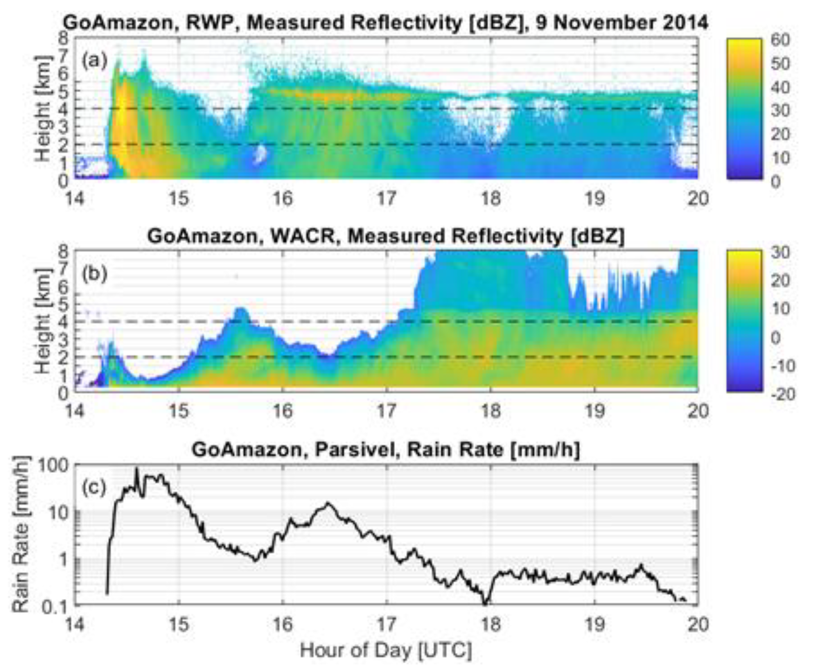
As the VPR operating frequency increases and enters the millimeter wave (mm-wave) operating wavelength region (i.e., 24 GHz frequency and higher, or 12.5 mm wavelength and shorter), rain attenuation significantly increases. At some combination of rain rate and path length, the return signal will be extinguished and the VPR will not detect raindrops nor ice particles above the rain shaft. For example, Figs. 1a and 1b show measured radar reflectivity factor [dBZ] profiles for a 6-h rain event collected by collocated 1.2 and 95 GHz VPRs operating near Manaus, Brazil (details of these data are provided in Section 2). The 1.2 GHz VPR observes high reflectivity between 2 and 4 km for about 10 min near 14:30 UTC indicating a convective core passing over the radar site. The 1.2 GHz VPR also observes a radar brightband at approximately 4.5 km height from hour 16 through 19 UTC indicating stratiform rain with snow and ice particles melting into raindrops.
In contrast, the 95 GHz VPR does not observe more than 1.5 km above the ground as the convective core passes overhead near 14:30 UTC. The 95 GHz VPR then observes rain below the 1.2 GHz VPR brightband during hour 16 UTC, but does not observe precipitation above 4 km. Then, after about mid-way through hour 17 UTC, the 95 GHz VPR begins to observe snow and ice particles above the 1.2 GHz VPR brightband. Figure 1c shows Parsivel disdrometer surface rain rate with values exceeding 20 mm h−1 as the convective core passes, rain rates are between 1 and 20 mm h−1 during hour 16 UTC, and rain rates are less than 1 mm h−1 after about mid-way through hour 17 UTC. Figure 1 illustrates that rainfall is severely attenuating the 95 GHz VPR signal and limiting valid VPR measurements above 4 km to periods with low surface rain rate precipitation. This severe attenuation raises this study’s main question: How far into a rain shaft can mm-wave VPRs detect raindrops?
To address this question, this study simulates rain shafts with a constant rain rate above a VPR and estimates how far into this rain shaft the VPR would produce valid observations. This calculation involves three main steps. The first step is to estimate the effective radar reflectivity factors and specific attenuations as a function of rain rate for different radar frequency bands. Next, attenuated radar reflectivity factor profiles are constructed for rain shafts with constant rain rate. The last step is to estimate the radar signal-to-noise ratio profiles for each rain shaft and estimate the range where the return signal is too weak to be detected by the VPR. Even though rain shafts in Nature do not have uniform rain rates, this simulation methodology enables a systematic approach to evaluate the performance of mm-wave VPRs used in precipitation and cloud studies.
This study has the following structure: Section 2 describes the VPR and surface disdrometer observations used in this study. Section 3 presents T-matrix raindrop scattering calculations needed to estimate radar effective reflectivity factor and specific attenuation. Section 3 also calculates power-law relationships between surface rain rate and both radar effective reflectivity factor and specific attenuation at eight radar bands (i.e., S-, C-, X-, Ku-, K-, Ka-, W-, and G-bands). Section 4 presents simulation results showing how far VPRs can observe into rain shafts. General conclusions are presented in Section 5.
2. Observations
This study uses observations collected during the US Department of Energy (DOE) Atmospheric Radiation Mission (ARM) Observations and Modeling of the Green Ocean Amazon (GOAmazon) field campaign from the Manaus, Brazil, field site [19]. Figure 1a shows reflectivity factor measurements from the 1.2 GHz Radar Wind Profiler (RWP) vertically pointing radar beam during a rain event on 9 November 2014 [20]. The RWP alternated beam pointing directions between vertical and two 15° off-vertical oblique beams pointed toward the North and East. The vertical beam observations are used for studying precipitation and the oblique beams are used to measure horizontal winds when it is not raining. Figure 1b shows measured reflectivity factor from the vertically pointing 95 GHz W-band ARM Cloud Radar (WACR) [21]. The WACR is sensitive enough to observe raindrops, ice particles, drizzle particles, and non-precipitating clouds [22]. A few pertinent RWP and WACR operating parameters during GOAmazon are listed in Table 1.
A surface Parsivel disdrometer measured the number and size of particles falling through a laser beam at 1-min resolution [23]. Observations were filtered to retain samples with Rayleigh reflectivity factor greater than 10 dBZ using raindrops from 24 diameter bins between 0.06 and 8.5 mm. There were 20,299 1-min samples meeting these criteria collected between September 2014 and November 2015. The surface rain rate for the 9 November 2014 rain event is shown in Figure 1c and is calculated using
where is the number concentration [number of raindrops with diameter m−3], is one of 24 Parsivel disdrometer diameter bins between 0.06 and 8.5 mm with resolution, and is the near surface terminal fall speed of a raindrop with diameter [24].
3. Methods
This section presents calculations needed for simulating VPR observations. Specifically, this section describes calculating raindrop backscattering and extinction cross-sections from T-matrix single raindrop scattering calculations which are used with the observed Parsivel disdrometer raindrop size distributions to estimate radar effective reflectivity factor and attenuation for radar operating frequencies ranging from 3 to 200 GHz. Power-law relationships are then derived representing mean characteristics between rain rate, radar reflectivity factor, and specific attenuation at each operating frequency. The atmospheric gaseous specific attenuation is approximated from oxygen and water vapor absorption calculated in global reference atmospheric models.
3.1. Raindrop Backscattering and Extinction Cross-Sections
The PyTmatrix Python module [25,26] was used to perform electromagnetic scattering calculations to estimate raindrop backscattering and extinction cross-sections at eight radar operating frequencies from 3 to 200 GHz. The PyTmatrix module calculates backscattering and extinction cross-sections for asymmetric raindrops at vertical and horizontal polarizations. However, when viewing raindrops at vertical incidence, as with VPRs, vertical and horizontal polarizations yield the same results due to symmetry.
For each numerical iteration, the PyTmatrix module was configured with a new set of input parameters, specifically: define the equivolumetric spherical raindrop diameter from 0.02 to 9.02 mm in 0.02 mm increments; define vertical incident wave propagation direction; define the radar operating frequency (see Table 2); define the complex dielectric constants of water at 0 °C and 20 °C (see Table 2); and define the approximate oblate spheroid shape with minor to major axis ratio [27]
Given a particular input parameter set, the PyTmatrix module produces the backscattering cross-section for each spherical raindrop in units mm2. To convert the backscattering cross-section to units of mm6 for radar reflectivity factor estimates, is normalization using
where is the water dielectric constant defined as .
Figure 2 shows the backscattering cross-section in decibel units and as a function of spherical diameter for the Rayleigh scattering approximation and the eight radar bands listed in Table 2. Note that backscattering resonance minima occur at spherical raindrop diameters of approximately 1.7 and 3 mm at W-band and at approximately 0.8, 1.34, and 1.9 mm at G-band.
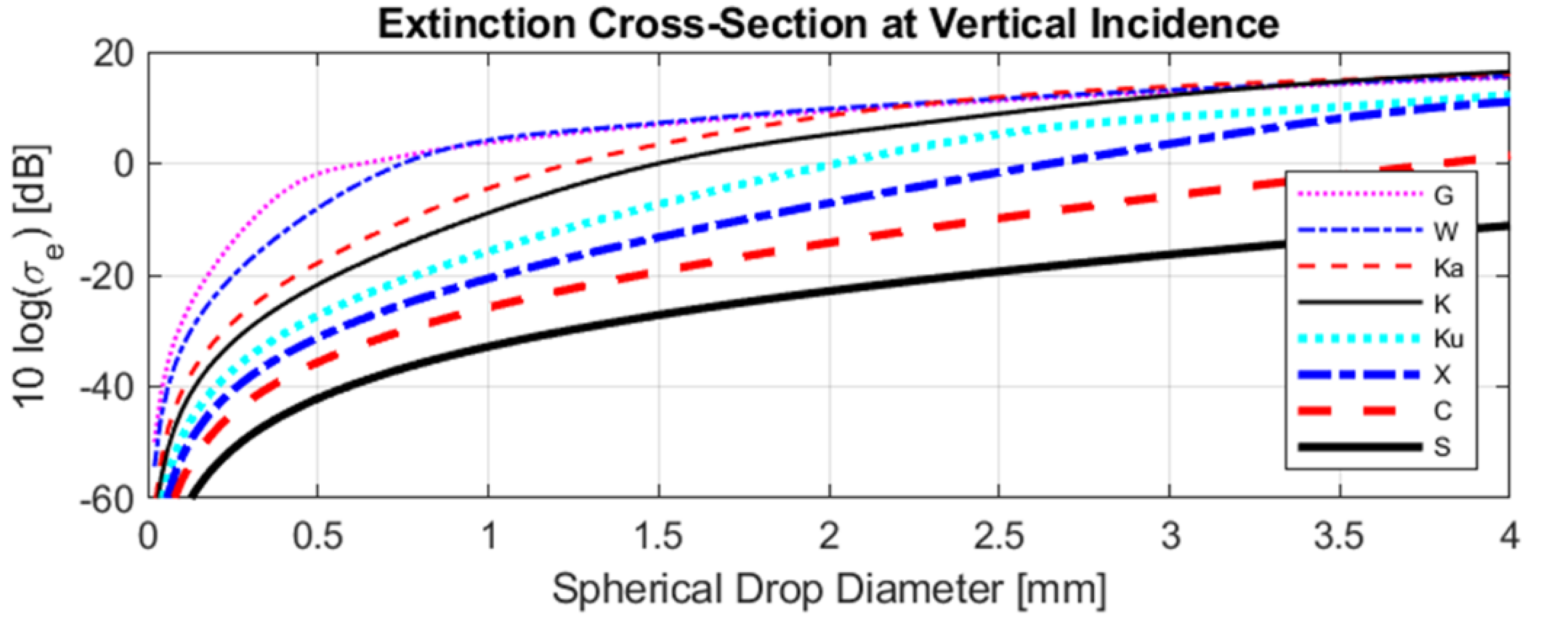
In addition to backscattering cross-section, the PyTmatrix module also estimates an extinction cross-section [mm2] for each raindrop. Figure 3 shows for eight radar bands as a function of equivolumetric spherical raindrop diameter .
The high diameter resolution PyTmatrix raindrop backscattering and extinction cross-sections were reduced to match the low resolution Parsivel disdrometer diameter bins so that radar effective reflectivity factor [mm6 m−3] and rain specific attenuation [dB km−1] can be estimated for each 1-min Parsivel number concentration and at each radar band using
and
Figure 4a shows Parsivel disdrometer radar effective reflectivity factor [dBZ] estimates assuming Rayleigh scattering and radar K-, Ka-, W-, and G-bands. In general, estimated radar effective reflectivity factors increase, approaching the Rayleigh scattering value, as the operating frequency decreases. Figure 4b shows Parsivel disdrometer derived rain specific attenuation [dB km−1] for radar K-, Ka-, W-, and G-bands. Note that W- and G-band rain specific attenuations are very similar, which is due to similar extinction cross-sections for raindrops larger than 0.8 mm diameter (see Figure 3). Though, as will be shown later, the addition of atmospheric gas attenuation causes different total attenuation profiles for these two frequency bands.
3.2. Power-Law Relationships for VPR Simulations
The previous section showed how disdrometer raindrop size distribution (DSD) measurements can be used to estimate specific attenuation [dB km−1], rain rate [mm h−1], and radar effective reflectivity factor [dBZ]. Minute-to-minute variation in measured DSD are helpful in studying the vertical structure and microphysical processes of individual rain events. Changes in DSD in the vertical are due to many processes, including evaporation, raindrop breakup/coalescence, and advection. In contrast, simulations of constant rain rate precipitation shifts (as presented in the next section) need just mean relationships between and as well as between and because minute-to-minute variations average to zero in the constant rain rate simulations. Thus, it is necessary to parameterize the mean radar reflectivity factor and mean rain specific attenuation at each radar frequency band as a function of rain rate. Parameterizations are developed using the GOAmazon field campaign Parsivel surface disdrometer measured rain rates , simulated radar effective reflectivity factors , and rain specific attenuations with power-law expressions of the form
and
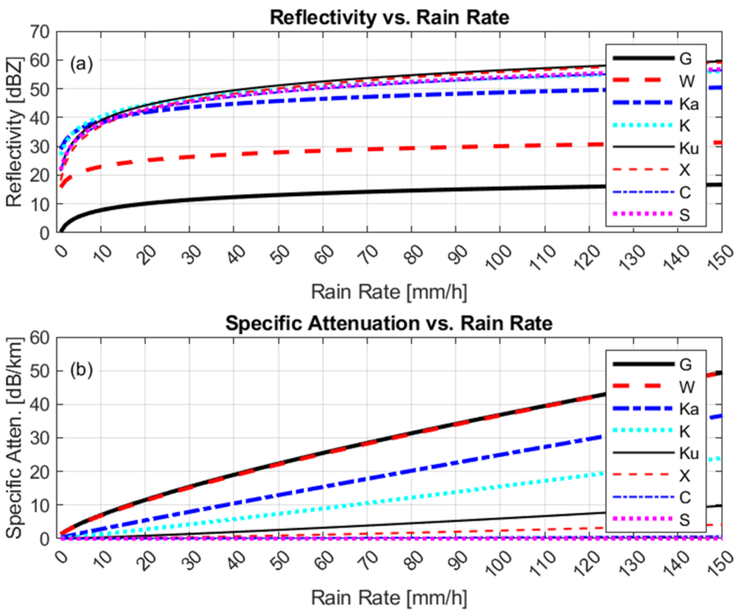
where coefficients , , , and are determined using a squared difference regression for each wavelength . Figure 5 shows the Parsivel estimated Ka-band effective reflectivity factor (Figure 5a) and rain specific attenuation (Figure 5b) versus the Parsivel rain rate with the color representing mass-weighted mean raindrop diameter ( [mm], where is the DSD moment). Note that for a constant rain rate, decreases as both reflectivity factor and specific attenuation increase. The solid lines in each panel are the power-law regressions. Figure 6 shows the -to- (Figure 6a) and -to- (Figure 6b) power-law regression lines for the eight radar frequency bands. Table 3 lists the coefficients for each power-law regression.
3.3. Specific Attenuation Due to Atmospheric Gases
The three main factors contributing to electromagnetic wave attenuation are scattering from precipitation particles (including raindrops and frozen particles), atmospheric gases, and non-precipitating cloud particles [28,29]. Gas attenuation magnitude increases with increasing operating frequency with significant losses at W- and G-bands. Thus, gas attenuation must be included in estimating the range where radar signals will be extinguished in rain shafts. Since clouds occur either near the top of rain shafts or isolated from falling particles, their attenuation contribution will be after the wave has already been affected by rain and gas attenuation. Thus, cloud particle attenuation is not addressed in this study, but will be a focus of future work.
Using the International Telecommunication Union (ITU) sea-level mean annual global reference atmosphere [30], approximate atmospheric gas specific attenuation due to oxygen and water vapor has been estimated to be from 1 GHz to 1 THz [31]. Table 4 lists near surface one-way atmospheric gas specific attenuation [dB km−1] at eight radar bands approximated by visually examining Figure 1 contained in [31].
4. Results
This section estimates how far a VPR can measure into a constant rain rate precipitation shaft following this three-step sequence: estimate attenuated radar reflectivity factor profile for a constant rain rate; convert an attenuated reflectivity factor profile into a radar signal-to-noise ratio profile; determine the range where the signal-to-noise ratio drops below the VPR’s detection limit.
4.1. Estimated Attenuated Radar Reflectivity Factor Profiles
The attenuated radar reflectivity factor, also known as the measured radar reflectivity factor [dBZ], at each range [m] from the radar is estimated from the non-attenuated effective reflectivity factor [dBZ] corrected for the 2-way path attenuation [dB] and can be expressed as [29]
The 2-way attenuation incorporates losses along the path from both rain and atmospheric gas specific attenuations and can be expressed as
where the factor 2 accounts for 2-way propagation, is the range to the range gate, the summations span from the first to the range gate with , and and are the rain and atmospheric gas specific attenuations at range . For the simulations used in this study, the rain columns have constant rain rate at all ranges and atmospheric gasses are assumed constant, which simplifies the path attenuation to
Furthermore, constant rain rate precipitation columns enable the measured reflectivity factor to be estimated from the surface rain rate using the previously derived -to- and -to- power-law relationships, yielding the expression
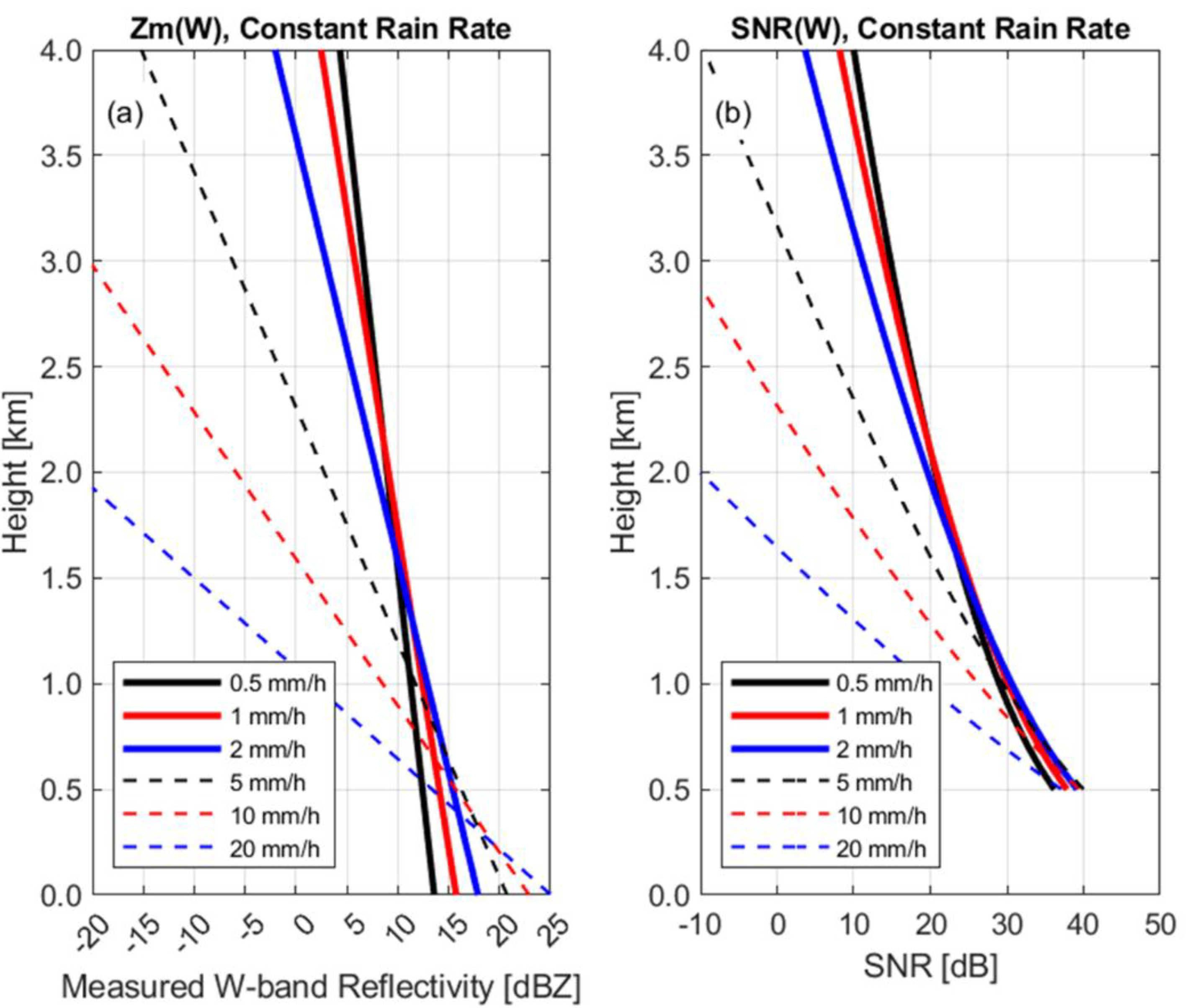
where coefficients , , , and were derived for each wavelength and are listed in Table 3. Note that for a constant rain rate column, the effective reflectivity factor is constant with range. Figure 7a shows profiles of estimated measured reflectivity at W-band for six surface rain rates of 0.5, 1, 2, 5, 10, and 20 mm h−1. The constant rain and gas specific attenuations with range causes constant slope profiles for each rain rate. Interestingly, due to attenuation between the surface and 500 m, the largest at 500 m occurred for the 5 mm h−1 rain rate.
4.2. Estimated Radar Signal-to-Noise Ratio Profiles
In order to simulate radar observations, the measured radar reflectivity factors shown in Figure 7a need to be converted to radar signal-to-noise ratios [unitless] to determine whether the return signals can be detected by the radar system. A simple monostatic pulse radar equation for volume scattering can be expressed as the received power over the noise power [16,32]
where is the transmitted power [W], is the antenna gain [unitless], is the electromagnetic wave propagation speed in air [m s−1], is the transmitted pulse length [s], and [radians] is the half-power antenna beamwidth that is squared under the assumption of a symmetric antenna pattern. Assuming a stable radar system with non-varying noise power, all of the parameters on the right-hand-side of Equation (12) are constant except for and . Thus, can be written as
where includes all constants in Equation (12). Expressing in decibels using , Equation (13) can be written as
where and is a radar calibration constant determined for each radar operating mode so that measured can be directly converted into [33]. In addition, scales the largest expected value to a value that will not saturate the radar receiver at some minimum range. Based on the WACR sensitivity analysis performed in the next sub-section, was determined to produce a maximum pre-saturation of 40 dB at a minimum range of 500 m. Figure 7b shows the corresponding profiles for the profiles shown in Figure 7a. Notice that decreases with range for all rain rates due to return power decreasing as for volume scattering (see Equations (12)–(14)). Specifically, decreases by 18 dB from 0.5 to 4 km due to this factor.
4.3. Maximum Range Based on Radar Receiver Dynamic Range
The radar receiver dynamic range is dependent on the radar design with radars operating in different modes to increase the overall radar dynamic range [4]. However, signal attenuation often prohibits the detection of thin clouds above highly attenuating rain columns even when using the more sensitive operating modes. The following analysis determines the simulation parameters needed to mimic the WACR performance as deployed for GOAmazon. To highlight the impact of wavelength dependent attenuation, all simulations used the same WACR parameterization.
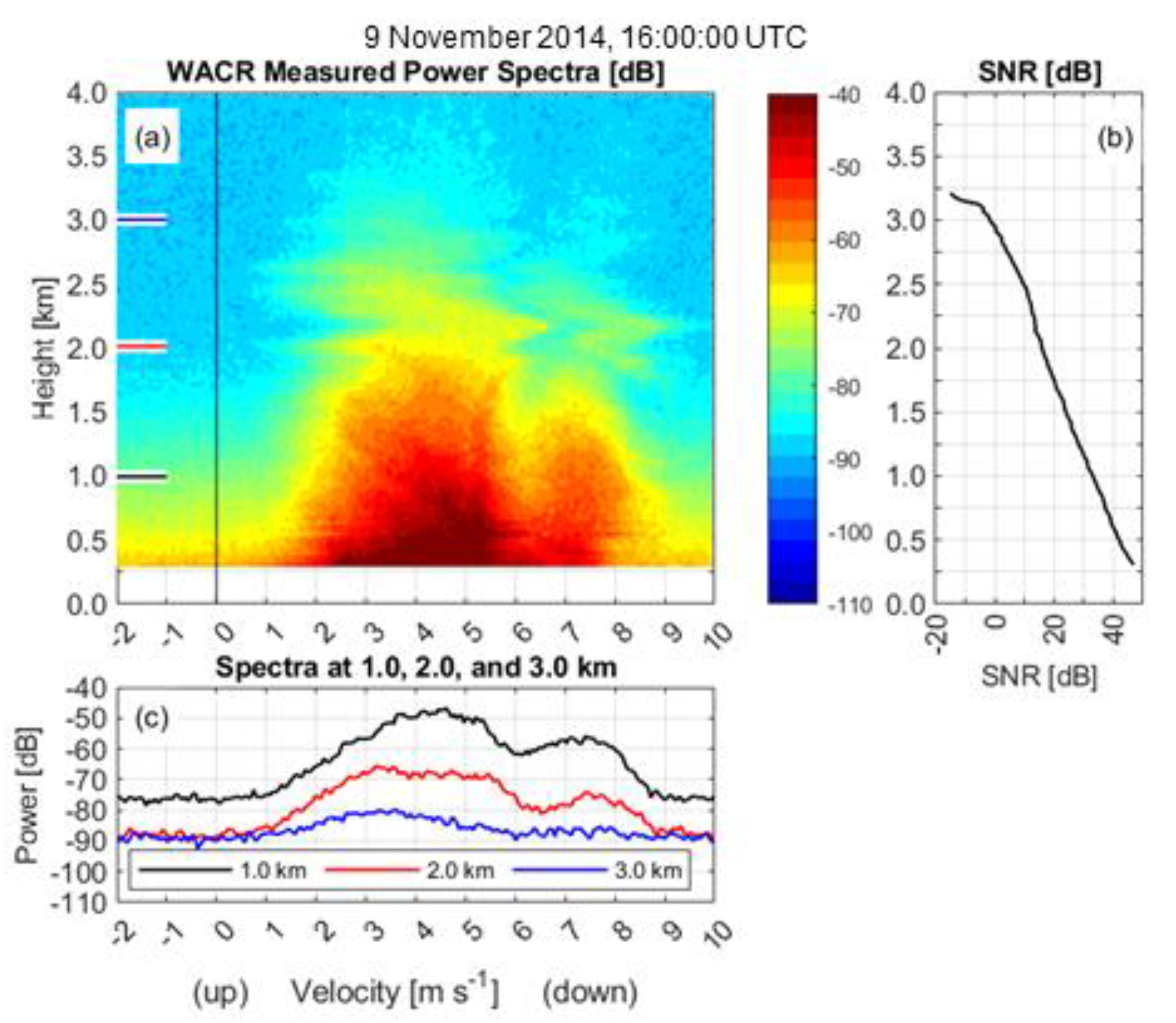
The WACR dynamic range during the GOAmazon field campaign can be estimated by examining Doppler velocity power spectra and profiles when attenuation is completely extinguishing the return signal. For example, a WACR profile is shown in Figure 8 from 9 November 2014 at 16:00:00 UTC as the surface Parsivel disdrometer measured 2.4 mm h−1 rain rate. Figure 8a shows the Doppler velocity power spectra profile, Figure 8b shows the at each range gate, and Figure 8c shows individual power spectra at ranges 1, 2, and 3 km. The at 0.5 km is approximately 40 dB (Figure 8b), drops to about 0 dB at 3.0 km, then abruptly drops to less than −10 dB. Figure 1a shows that the RWP 1.2 GHz VPR is observing a radar brightband at 4.7 km at 16:00 UTC. Combining information from Figure 1 and Figure 8 suggests that the WACR 95 GHz return signal is being completely extinguished by rain attenuation.
The individual power spectra at 1 and 2 km (Figure 8c) show well defined bi-modal peaks due to the backscattering resonance minimum near 1.7 mm diameter raindrops (see Figure 2b). Yet, the bi-modality is not as well defined in the spectrum from 3 km because of the lower . Visual inspection of the spectra profile (Figure 8a) suggest that bi-modal spectra can be visually identified at ranges below 3 km. Thus, from this analysis, the lowest usable for this radar deployment is about 0 dB. Using the at 0.5 km range as a reference, the receiver dynamic range for this radar deployment is about 40 dB.
Turning back to Figure 7b which shows simulated profiles for constant rain rate precipitation shafts, the calibration constant was selected to match the WACR determined maximum pre-saturation of 40 dB at 500 m. A 40 dB dynamic range implies this VPR can detect raindrops at all ranges until the drops below 0 dB. In Figure 7b, the drops to 0 dB at approximately 1.7, 2.3, and 3.2 km for rain rates of 20, 10, and 5 mm h−1, respectively.
Figure 9a,b show the observed WACR and the simulated profiles for the 09 November 2014 rain event. The simulated W-band profiles are derived from the surface rain rate by first estimating measured reflectivity factor profiles using Equation (11) and then converting to profiles using Equation (14). The minimum values plotted in Figure 9a,b are limited to −7 dB. The Parsivel disdrometer surface rain rates used to construct the simulated profiles are shown in Figure 9c. The red circles in Figure 9a,b correspond to the range when the simulated drops to 0 dB. During hours 14–17, when the rain rates exceed 1 mm h−1, the red circles, in general, track the minimum observed shown in Figure 9a. Though, during hour 15, the red circles are higher in height indicating that there is more attenuation, or a decrease in , in the observations (Figure 9a) compared to the simulated constant rain rate profiles (Figure 9b). However, overall, the agreement is good enough to estimate how far WACR would measure into rain during the GOAmazon field campaign.
4.4. Simulated Maximum Range into Constant Rain Rate Shafts at Multiple Radar Bands
To highlight how attenuation depends on radar operating frequency, the simulation parameters derived to mimic the WACR as deployed in GoAmazon are used in the simulations for the other seven operating frequencies. Specifically, it is assumed that the radar receiver has 40 dB dynamic range and the maximum of 40 dB occurs at 500 m. Figure 10 shows the maximum height coverage versus rain rate for the K-, Ka-, W-, and G-bands for calculations including both rain and atmospheric gas attenuation. Focusing first on the simulated WACR sensitivity, the W-band curve in Figure 10 indicates that in order for WACR to observe above a 2.0 km column of rain, the rain rate in that column must be less than 14 mm h−1. Assuming the WACR simulation parameters are applied to K-, Ka-, and G-band radars, those radars would observe above 2.0 km for rain rates less than approximately 60, 33, and 9 mm h−1, respectively.
To help compare how far mm-wave VPRs can measure rain into constant rain rate precipitation columns, Table 5 lists the rain rates needed to extinguish the return signal as a function of path length and radar band. Thus, this table indicates that in order to measure rain beyond a rain column 3.5 km deep, the rain rate must be less than 138, 67, 26, 14, and 4 mm h−1 for radar X-, Ku-, K-, Ka-, and W-bands. Due solely to atmospheric gas attenuation, the radar G-band return signal will be completely extinguished by 3.5 km. Therefore, a G-band VPR will not detect any rain above 3.5 km, independent of rain shaft rain rate.
4.5. Observed Maximum WACR Range versus Observed Surface Rain Rate
One way to check the WACR simulated maximum height through rain shafts is to analyze the observed maximum WACR heights partitioned by the observed surface rain rate. Between September 2014 and November 2015, the Parsivel disdrometer measured over 16,700 min of rain rate larger than 0.5 mm h−1. For each minute, the WACR profiles were analyzed to determine the height where the dropped below the detection limit. With approximately 30 WACR profiles per minute, there were over 370,000 WACR profiles associated with observed surface rain rates. Figure 11a shows box whisker plots of the maximum observed WACR height as a function of the surface rain rate. The 25-to-75 percentiles are shown with the black boxes, the 50% median is represented with the horizontal line within the box, and the 10 and 90 percentiles are indicated as the whisker tips. Figure 11b indicates the number of WACR profiles for each rain rate.
The blue solid line in Figure 11a is the simulated W-band WACR maximum height also shown in Figure 10. The simulated maximum heights fall between the observed 25 and 50 percentiles for all simulated rain rates. The higher observed maximum heights are probably due to the assumed constant rain rate in the simulations as well as variations in DSD with height due to microphysical processes including raindrop breakup and coalescence.
5. Conclusions
This study explored the question: How far into a rain shaft can a mm-wave vertically pointing radar (VPR) detect raindrops before the attenuation is so severe that the return signal is extinguished? Since attenuation is the product of path length and specific attenuation, the experimental design systematically varied the rain rate to produce constant specific attenuation rain shafts and then estimated the path length that attenuated the return signal so much that the signal-to-noise ratio dropped below the VPR’s detection limit. This study used surface disdrometer observations and publicly available T-matrix scattering code to produce realistic radar reflectivity factor profiles at different radar operating bands from 3 to 200 GHz. These simulated profiles were converted into VPR profiles and then used to determine when the return signal was no longer detectable by the VPR. By varying the rain rate of the simulated rain shafts, the maximum path length that extinguished the return signal was estimated as a function of rain rate for each operating frequency.
The simulation parameters were derived to mimic the U.S. Department of Energy Atmospheric Radiation Mission (ARM) W-band radar (WACR) as it was deployed in the GoAmazon field campaign. To highlight how attenuation is dependent on radar operating frequency, the simulations for the other radar bands used the same WACR derived simulation parameters. Specifically, the simulations assumed a radar receiver with 40 dB dynamic range and the maximum of 40 dB at 500 m. Details are provided herein for determining these simulation parameters for other radar systems.
The W-band simulated maximum heights were collaborated with observed W-band WACR heights partitioned by surface Parsivel disdrometer rain rates. The simulated maximum height was between the 25 and 50 percentiles of the observed maximum heights. The observed heights are postulated to be higher because the simulations assumed constant rain rate while natural rain varied with height.
This study found that the primary factors limiting mm-wave VPRs from observing into rain shafts include: (1) rain and atmospheric gas attenuation, (2) return power decreasing as for volume scattering, and (3) radar receiver dynamic range.
Concerning rain and atmospheric gas attenuation, this study isolated the two attenuation factors so that they can be adjusted independently, as needed, to account for VPR deployments in other field campaigns. The simulations indicate that for a radar to observe above 3.5 km, the rain rate of rain shafts must be less than 26, 14, and 4 mm h−1 for K-, Ka, and W-bands, respectively (see Table 5). Compared to observations, the W-band WACR maximum heights ranged between 3 and 4.5 km when the surface disdrometer measured 4 mm hr−1 rain rate, which are based on 25-to-75 percentiles from over 25,000 W-band radar profiles. The severe attenuation at low rain rates limits W-band observations to low altitudes in convective cloud studies [13].
While the rain attenuation is not location dependent, gas attenuation is dependent on water vapor amount. To produce general and repeatable results, this study used International Telecommunication Union (ITU) reference atmosphere and near-surface gas attenuation calculations [30,31]. These gas attenuations will need to be adjusted for different deployment locations. In particular, the reference ITU gas attenuation at G-band is so severe that a rain-free path length of 3.5 km will completely extinguish the return signal. Rain attenuation will contribute to reducing this path length, further limiting G-band ground-based VPR measurements to close range.
The decrease in return power due to the range squared factor (i.e., ) for volume scattering is important for near radar observations. This factor causes an 18 dB decrease in as range changes from 0.5 to 4 km. Whereas a 3.5 km change in range from 6.5 to 10 km only causes a 3.7 dB decease. This decrease in radar sensitivity is independent of rain rate.
The radar receiver dynamic range is an important factor in balancing the tradeoff between not saturating at close range and making low measurements at far ranges. This study found that the WACR system deployed during GOAmazon had a 40 dB dynamic range. Increasing the dynamic range in future radar hardware will increase the path length mm-wave VPRs will be able to measure through rain shafts.
In summary, this study contributes to our understanding of how rain and atmospheric gas attenuation impacts the performance of mm-wave VPRs and will help with the design and configuration of multi-frequency VPRs deployed in future field campaigns.
Funding
This research was supported by the U.S. Department of Energy’s Atmospheric System Research, an Office of Science Biological and Environmental Research program, under Grant No. DE-SC0021345.
Data Availability Statement
The datasets used in this study are available from the DOE ARM Archive with specific DOIs for each data stream provided in the references. Section 3.1 contains enough information to run the Python PyTmatrix module and recalculate the backscattering and extinction cross-sections used in this study.
Acknowledgments
The author acknowledges insightful conversations with colleagues Joseph Hardin (Pacific Northwest National Laboratory), Haonan Chen (Colorado State University), and Chris Fairall (NOAA Earth System Research Laboratory) for our discussions on T-matrix calculations and attenuation estimates.
Conflicts of Interest
The author declares no conflict of interest.
References
- Ecklund, W.L.; Gage, K.S.; Williams, C.R. Tropical precipitation studies using a 915-MHz wind profiler. Radio Sci. 1995, 30, 1055–1064. [Google Scholar] [CrossRef]
- Ecklund, W.L.; Williams, C.R.; Johnston, P.E.; Gage, K.S. A 3-GHz Profiler for Precipitating Cloud Studies. J. Atmos. Ocean. Technol. 1999, 16, 309–322. [Google Scholar] [CrossRef]
- Kollias, P.; Clothiaux, E.E.; Miller, M.A.; Albrecht, B.A.; Stephens, G.L.; Ackerman, T.P. Millimeter-wavelength radars: New frontier in atmospheric cloud and precipitation research. Bull. Amer. Meteor. Soc. 2007, 88, 1608–1624. [Google Scholar] [CrossRef] [Green Version]
- Kollias, P.; Bharadwaj, N.; Clothiaux, E.E.; Lamer, K.; Oue, M.; Hardin, J.; Isom, B.; Lindenmaier, I.; Matthews, A.; Luke, E.P.; et al. The ARM radar network: At the leading edge of cloud and precipitation observations. Bull. Amer. Meteor. Soc. 2020, 101, E588–E660. [Google Scholar] [CrossRef] [Green Version]
- Görsdorf, U.; Lehmann, V.; Bauer-Pfundstein, M.; Peters, G.; Vavriv, D.; Vinogradov, V.; Volkov, V. A 35-GHz polarimetric doppler radar for long-term observations of cloud parameters-description of system and data processing. J. Atmos. Ocean. Technol. 2015, 32, 675–690. [Google Scholar] [CrossRef]
- Battaglia, A.; Kollias, P. Evaluation of differential absorption radars in the 183 GHz band for profiling water vapour in ice clouds. Atmos. Meas. Tech. 2019, 12, 1–18. [Google Scholar] [CrossRef] [Green Version]
- Battaglia, A.; Courtier, B.; Huggard, P.; Mroz, K. First observations of multi-frequency radar Doppler spectra including a G-band (200 GHz) radar. In Proceedings of the American Geophysical Union Annual Fall Meeting, New Orleans, LA, USA, 13–17 December 2021. [Google Scholar]
- Lhermitte, R.M. Cloud and Precipitation Remote Sensing at 94 GHz. IEEE Trans. Geosci. Remote Sens. 1988, 26, 207–216. [Google Scholar] [CrossRef]
- Lhermitte, R.M. Observation of rain at vertical incidence with a 94 GHz Doppler radar: An insight on Mie scattering. Geophys. Res. Lett. 1988, 15, 1125–1128. [Google Scholar] [CrossRef]
- Giangrande, S.E.; Babb, D.M.; Verlinde, J. Processing Millimeter Wave Profiler Radar Spectra. J. Atmos. Ocean. Technol. 2001, 18, 1577–1583. [Google Scholar] [CrossRef]
- Giangrande, S.E.; Luke, E.P.; Kollias, P. Automated retrievals of precipitation parameters using non-Rayleigh scattering at 95 GHz. J. Atmos. Ocean. Technol. 2010, 27, 1490–1503. [Google Scholar] [CrossRef]
- Giangrande, S.E.; Luke, E.P.; Kollias, P. Characterization of vertical velocity and drop size distribution parameters in widespread precipitation at ARM facilities. J. Appl. Meteor. Climatol. 2012, 51, 380–391. [Google Scholar] [CrossRef] [Green Version]
- Kollias, P.; Lhermitte, R.; Albrecht, B.A. Vertical air motion and raindrop size distributions in convective systems using a 94 GHz radar. Geophys. Res. Lett. 1999, 26, 3109–3112. [Google Scholar] [CrossRef]
- Williams, C.R. Vertical air motion retrieved from dual-frequency profiler observations. J. Atmos. Ocean. Technol. 2012, 29, 1471–1480. [Google Scholar] [CrossRef]
- Tridon, F.; Battaglia, A. Dual-frequency radar doppler spectral retrieval of rain drop size distributions and entangled dynamics variables. J. Geophys. Res. 2015, 120, 5585–5601. [Google Scholar] [CrossRef] [Green Version]
- Bringi, V.N.; Chandrasekar, V. Polarimetric Doppler Weather Radar; Cambridge University Press: Cambridge, UK, 2001; p. 636. [Google Scholar]
- Williams, C.R.; Beauchamp, R.M.; Chandrasekar, V. Vertical Air Motions and Raindrop Size Distributions Estimated Using Mean Doppler Velocity Difference from 3-and 35-GHz Vertically Pointing Radars. IEEE Trans. Geosci. Remote Sens. 2016, 54, 6048–6060. [Google Scholar] [CrossRef]
- Kneifel, S.; Moisseev, D. Long-term statistics of riming in nonconvective clouds derived from ground-based doppler cloud radar observations. J. Atmos. Sci. 2020, 77, 3495–3508. [Google Scholar] [CrossRef]
- Martin, S.T.; Artaxo, P.; Machado, L.; Manzi, A.O.; Souza, R.A.F.; Schumacher, C.; Wang, J.; Biscaro, T.; Brito, J.; Calheiros, A.; et al. The Green Ocean Amazon experiment (GOAmazon 2014/5) observes pollution affecting gases, aerosols, clouds, and rainfall over the rain forest. Bull. Amer. Meteor. Soc. 2017, 98, 981–997. [Google Scholar]
- Coulter, R.; Muradyan, P.; Martin, T. Atmospheric Radiation Measurement (ARM) User Facility, Radar Wind Profiler (1290RWPPRECIPSPEC). 2014-11-09, ARM Mobile Facility (MAO) Manacapuru, Amazonas, Brazil; AMF1 (M1). 2014. Available online: http://0-dx-doi-org.brum.beds.ac.uk/10.5439/1502660 (accessed on 12 May 2016).
- Bharadwaj, N.; Lindenmaier, I.; Johnson, K.; Nelson, D.; Matthews, A. Atmospheric Radiation Measurement (ARM) User Facility, W-Band (95 GHz) ARM Cloud Radar (WACRSPECCMASKCOPOL). 2014-09-25 to 2015-12-01, ARM Mobile Facility (MAO) Manacapuru, Amazonas, Brazil; AMF1 (M1). 2014. Available online: http://0-dx-doi-org.brum.beds.ac.uk/10.5439/1025318 (accessed on 14 May 2016).
- Mather, J.; Voyles, J. The ARM climate research facility: A review of structure and capabilities. Bull. Amer. Meteorol. Soc. 2013, 94, 377–392. [Google Scholar] [CrossRef]
- Wang, D.; Bartholomew, M.; Shi, Y. Atmospheric Radiation Measurement (ARM) User Facility, Laser Disdrometer (LD). 2014-09-25 to 2015-12-01, ARM Mobile Facility (MAO) Manacapuru, Amazonas, Brazil, Supplemental Site (S10). 2014. Available online: http://0-dx-doi-org.brum.beds.ac.uk/10.5439/1779709 (accessed on 20 February 2018).
- Gunn, R.; Kinzer, G.D. The terminal velocity of fall for water drops in stagnant air. J. Meteorol. 1949, 6, 243–248. [Google Scholar] [CrossRef] [Green Version]
- Leinonen, J. High-level interface to T-matrix scattering calculations: Architecture, capabilities and limitations. Optics Express 2014, 22, 1655–1660. [Google Scholar] [CrossRef]
- Leinonen, J. Python Code for T-Matrix Scattering Calculations. Available online: https://github.com/jleinonen/pytmatrix/ (accessed on 1 October 2021).
- Thurai, M.; Huang, G.J.; Bringi, V.N.; Randeu, W.L.; Schönhuber, M. Drop shapes, model comparisons, and calculations of polarimetric radar parameters in rain. J. Atmos. Ocean. Technol. 2007, 24, 1019–1032. [Google Scholar] [CrossRef]
- Pujol, O.; Georgis, J.F.; Féral, L.; Sauvageot, H. Degradation of radar reflectivity by cloud attenuation at microwave frequency. J. Atmos. Ocean. Technol. 2007, 24, 640–657. [Google Scholar] [CrossRef]
- Li, L.; Sekelsky, S.M.; Reising, S.C.; Swift, C.T.; Durden, S.L.; Sadowy, G.A.; Dinardo, S.J.; Li, F.K.; Huffman, A.; Stephens, G.; et al. Retrieval of Atmospheric Attenuation Using Combined Ground-Based and Airborne 95-GHz Cloud Radar Measurements. J. Atmos. Ocean. Technol. 2001, 18, 1345–1353. [Google Scholar] [CrossRef] [Green Version]
- ITU-R. Recommendation ITU-R P.835-6 (12/2017) Reference Standard Atmospheres. International Telecommunication Union, 2017. Available online: https://www.itu.int/rec/R-REC-P.835 (accessed on 8 January 2022).
- ITU-R. Recommendation ITU-R P.676-12 (08/2019) Attenuation by Atmospheric Gases and Related Effects. International Telecommunication Union, 2019. Available online: https://www.itu.int/rec/R-REC-P.676 (accessed on 8 January 2022).
- Küchler, N.; Kneifel, S.; Löhnert, U.; Kollias, P.; Czekala, H.; Rose, T. A W-band radar-radiometer system for accurate and continuous monitoring of clouds and precipitation. J. Atmos. Ocean. Technol. 2017, 34, 2375–2392. [Google Scholar] [CrossRef]
- Hartten, L.M.; Johnston, P.E.; Castro, V.M.R.; Pérez, P.S.E. Postdeployment calibration of a tropical UHF profiling radar via surface-and satellite-based methods. J. Atmos. Ocean. Technol. 2019, 36, 1729–1751. [Google Scholar] [CrossRef]
Figure 1.
Measured radar reflectivity factor from vertically pointing radars (VPRs) deployed near Manaus, Brazil, during the DOE GOAmazon field campaign from an event on 9 November 2014. (a) Radar Wind Profiler (RWP) operating at 1.2 GHz and (b) W-band ARM Cloud Radar (WACR) operating at 95 GHz. (c) Surface Parsivel disdrometer rain rate.

Figure 2.
Normalized backscattering cross-section at vertical incidence expressed in decibel units verses equivolumetric spherical raindrop diameter . (a) Rayleigh scattering regime and radar S-, C-, and X-bands. (b) Radar Ku-, K-, Ka-, W-, and G-bands.
Figure 2.
Normalized backscattering cross-section at vertical incidence expressed in decibel units verses equivolumetric spherical raindrop diameter . (a) Rayleigh scattering regime and radar S-, C-, and X-bands. (b) Radar Ku-, K-, Ka-, W-, and G-bands.

Figure 3.
Extinction cross-section at vertical incidence expressed in decibel units verses spherical raindrop diameter for radar S-, C-, X-, Ku-, K-, Ka-, W-, and G-bands.
Figure 3.
Extinction cross-section at vertical incidence expressed in decibel units verses spherical raindrop diameter for radar S-, C-, X-, Ku-, K-, Ka-, W-, and G-bands.

Figure 4.
Surface Parsivel disdrometer derived radar effective reflectivity factor and rain specific attenuation. (a) Radar effective reflectivity factor assuming Rayleigh scattering and scattering at K-, Ka-, W-, and G-bands; (b) rain specific attenuation at radar K-, Ka-, W-, and G-bands.
Figure 4.
Surface Parsivel disdrometer derived radar effective reflectivity factor and rain specific attenuation. (a) Radar effective reflectivity factor assuming Rayleigh scattering and scattering at K-, Ka-, W-, and G-bands; (b) rain specific attenuation at radar K-, Ka-, W-, and G-bands.

Figure 5.
Relationships between surface Parsivel disdrometer derived rain rate, radar effective reflectivity factor, and rain specific attenuation. (a) Radar Ka-band effective reflectivity factor [dBZ] versus rain rate [mm h−1] with colors indicating [mm]. (b) Radar Ka-band rain specific attenuation [dB km−1] versus rain rate [mm h−1] with colors indicating [mm]. The regression lines are power-law fits of the form (6) and (7) with coefficients listed in Table 3.

Figure 6.
Power-law relationships of the form (6) and (7) derived from Parsivel measured raindrop size distributions for radar S-, C-, X-, Ku-, K-, Ka-, W-, and G-bands. (a) Radar effective reflectivity factor [dBZ] versus rain rate [mm h−1]; (b) rain specific attenuation [dB km−1] versus rain rate [mm h−1]. Power law coefficients are listed in Table 3.

Figure 7.
Estimated W-band measured reflectivity and as a function of range for rain shafts with constant rain rates of 0.5, 1, 2, 5, 10, and 20 mm h−1. (a) Simulated measured reflectivity factor [dBZ] and (b) signal-to-noise ratio [dB].
Figure 7.
Estimated W-band measured reflectivity and as a function of range for rain shafts with constant rain rates of 0.5, 1, 2, 5, 10, and 20 mm h−1. (a) Simulated measured reflectivity factor [dBZ] and (b) signal-to-noise ratio [dB].

Figure 8.
WACR measured Doppler velocity power spectra profile from 9 November 2014 at 16:00:00 UTC with surface rain rate of 2.4 mm h−1. (a) Power spectra from 0.3 to 4 km with color representing power intensity [dB] (downward motion has positive velocity), (b) signal-to-noise ratio [dB], and (c) individual power spectra from 1, 2, and 3 km heights [dB].

Figure 9.
Time-height cross-section of W-band SNR. (a) Measured WACR [dB] on 9 November 2014, (b) simulated SNR [dB] derived from surface rain rate (see Equations (11) and (14)). The two black dashed lines at 4 and 2 km are visual aids to facilitate comparing panels. Red circles correspond to the height where the simulated SNR in (b) is 0 dB. (c) Surface disdrometer rain rate used to construct simulated SNR profiles in (b).

Figure 10.
Estimated maximum VPR path length as a function of constant rain rate and for radar K-, Ka-, W-, and G-bands. Maximum height is defined when the drops 40 dB from the maximum pre-saturation observed at 500 m. Simulation parameters mimic W-band WACR as deployed in GoAmazon.
Figure 10.
Estimated maximum VPR path length as a function of constant rain rate and for radar K-, Ka-, W-, and G-bands. Maximum height is defined when the drops 40 dB from the maximum pre-saturation observed at 500 m. Simulation parameters mimic W-band WACR as deployed in GoAmazon.

Figure 11.
Observed WACR maximum height as a function of simultaneous surface rain rate. (a) Box whisker plot of observed WACR maximum height, center line is median, box edges are 25 and 75 percentiles, and whisker tips are 10 and 90 percentiles. The blue line is the simulated W-band WACR maximum height shown in Figure 10. (b) Number of WACR profiles for each surface Parsivel disdrometer rain rate. Over 370,000 WACR profiles were observed when Parsivel disdrometer rain rates were greater than 0.5 mm h−1 between September 2014 and November 2015.


Table 1.
Pertinent Radar Wind Profiler (RWP) and W-band ARM Cloud Radar (WACR) operating parameters during the GOAmazon field campaign.
Table 1.
Pertinent Radar Wind Profiler (RWP) and W-band ARM Cloud Radar (WACR) operating parameters during the GOAmazon field campaign.
| Parameter | RWP | WACR |
|---|---|---|
| Operating Frequency | 1.2 GHz | 95 GHz |
| Operating Wavelength | 250 mm | 3.2 mm |
| Distance between Range Gates | 225 m | 30 m |
| Range to First Range Gate | 510 m | 300 m |
| Range to Last Range Gate | 17 km | 18 km |
| Dwell Time | 2 s | 2 s |
| Time between Samples | 12 s | 2 s |
Table 2.
Wavelength dependent complex dielectric constant and squared water dielectric constant at 0° and 20 °C that are needed as inputs to the PyTmatrix module. Additional non-wavelength dependent input parameters needed for the PyTmatrix module include: raindrop spherical diameters from 0.02 to 9.02 mm in 0.02 increments, raindrop obliqueness relationship of Equation (2), and simulations performed at vertical incidence.
| Band | Wavelength [mm] | m (0 °C) | (0 °C) | m (20 °C) | (20 °C) |
|---|---|---|---|---|---|
| S (2.7 GHz) | 111.0 | 9.092 + 1.266i | 0.934 | 8.875 + 0.675i | 0.928 |
| C (5.6 GHz) | 53.6 | 8.340 + 2.226i | 0.933 | 8.615 + 1.315i | 0.928 |
| X (9 GHz) | 33.3 | 7.364 + 2.805i | 0.930 | 8.176 + 1.910i | 0.927 |
| Ku (13.6 GHz) | 22.1 | 6.329 + 2.977i | 0.925 | 7.502 + 2.392i | 0.924 |
| K (24 GHz) | 12.5 | 4.876 + 2.803i | 0.908 | 6.201 + 2.807i | 0.918 |
| Ka (35.6 GHz) | 8.4 | 4.033 + 2.438i | 0.879 | 5.192 + 2.779i | 0.908 |
| W (94 GHz) | 3.1 | 2.819 + 1.387i | 0.688 | 3.372 + 1.935i | 0.815 |
| G (200 GHz) | 1.5 | 2.448 + 0.749i | 0.482 | 2.668 + 1.174i | 0.622 |
Table 3.
Power-law coefficients for -to- and -to- relationships with the form and . Radar effective reflectivity factor has units [mm6 m−3], rain specific attenuation has units [dB km−1], and rain rate has units [mm h−1].
Table 3.
Power-law coefficients for -to- and -to- relationships with the form and . Radar effective reflectivity factor has units [mm6 m−3], rain specific attenuation has units [dB km−1], and rain rate has units [mm h−1].
| Band | Wavelength [mm] | ||||
|---|---|---|---|---|---|
| S (2.7 GHz) | 111.0 | 150 | 1.610 | 2.28 × 10−04 | 1.038 |
| C (5.6 GHz) | 53.6 | 144 | 1.599 | 7.88 × 10−04 | 1.349 |
| X (9 GHz) | 33.3 | 64.5 | 1.884 | 4.18 × 10−03 | 1.380 |
| Ku (13.6 GHz) | 22.1 | 139 | 1.749 | 2.35 × 10−02 | 1.203 |
| K (24 GHz) | 12.5 | 489 | 1.340 | 0.110 | 1.075 |
| Ka (35.6 GHz) | 8.4 | 781 | 0.988 | 0.320 | 0.946 |
| W (94 GHz) | 3.1 | 37.5 | 0.716 | 1.26 | 0.732 |
| G (200 GHz) | 1.5 | 1.06 | 0.756 | 1.32 | 0.723 |
Table 4.
Near surface one-way atmospheric gas specific attenuation [dB km−1] at each radar band approximated by visually examining Figure 1 contained in [31]. Estimates in [31] assume ITU reference atmosphere [30] of 1013.25 hPa pressure, 15 °C temperature, and 7.5 g m−3 water vapor density.
| S- | C- | X- | Ku- | K- | Ka- | W- | G- |
|---|---|---|---|---|---|---|---|
| 0.008 | 0.009 | 0.01 | 0.03 | 0.15 | 0.1 | 0.4 | 3 |
Table 5.
Rain rates [mm h−1] of constant rain rate precipitation shafts that extinguish the return signal for different path lengths and for radar X-, Ku-, K-, Ka-, W-, and G-bands. Calculations based on 40 dB radar receiver dynamic range with maximum observed at 500 m. Simulation parameters mimic W-band WACR as deployed in GoAmazon and include atmospheric gas attenuation in the ITU reference atmosphere.
| Path Length | X-Band | Ku-Band | K-Band | Ka-Band | W-Band | G-Band |
|---|---|---|---|---|---|---|
| 4.0 km | 116 | 55 | 21 | 11 | 3 | -1. |
| 3.5 km | 138 | 67 | 26 | 14 | 4 | -1. |
| 3.0 km | 166 | 84 | 33 | 18 | 6 | 1 |
| 2.5 km | >200 | 107 | 44 | 24 | 9 | 4 |
| 2.0 km | >200 | 142 | 60 | 33 | 14 | 9 |
1. Return signal completely extinguished due to atmospheric gas attenuation.
Publisher’s Note: MDPI stays neutral with regard to jurisdictional claims in published maps and institutional affiliations. |
© 2022 by the author. Licensee MDPI, Basel, Switzerland. This article is an open access article distributed under the terms and conditions of the Creative Commons Attribution (CC BY) license (https://creativecommons.org/licenses/by/4.0/).
Share and Cite
MDPI and ACS Style
Williams, C.R. How Much Attenuation Extinguishes mm-Wave Vertically Pointing Radar Return Signals? Remote Sens. 2022, 14, 1305. https://0-doi-org.brum.beds.ac.uk/10.3390/rs14061305
AMA Style
Williams CR. How Much Attenuation Extinguishes mm-Wave Vertically Pointing Radar Return Signals? Remote Sensing. 2022; 14(6):1305. https://0-doi-org.brum.beds.ac.uk/10.3390/rs14061305
Chicago/Turabian StyleWilliams, Christopher R. 2022. "How Much Attenuation Extinguishes mm-Wave Vertically Pointing Radar Return Signals?" Remote Sensing 14, no. 6: 1305. https://0-doi-org.brum.beds.ac.uk/10.3390/rs14061305
Note that from the first issue of 2016, this journal uses article numbers instead of page numbers. See further details here.