
Long-Term Vegetation Phenology Changes and Responses to Preseason Temperature and Precipitation in Northern China


1
Fujian Provincial Key Laboratory of Remote Sensing of Soil Erosion, College of Environment & Safety Engineering, Fuzhou University, Fuzhou 350116, China
2
Earth System Science Interdisciplinary Center, University of Maryland, College Park, MD 20740, USA
3
School of Life Sciences, University of Technology Sydney, Sydney 2007, Australia
4
Key Lab of Spatial Data Mining & Information Sharing, Ministry of Education of China, Fuzhou 350116, China
*
Author to whom correspondence should be addressed.
Remote Sens. 2022, 14(6), 1396; https://0-doi-org.brum.beds.ac.uk/10.3390/rs14061396
Submission received: 18 February 2022
/
Revised: 8 March 2022
/
Accepted: 11 March 2022
/
Published: 14 March 2022
(This article belongs to the Special Issue Remote Sensing for Crop Stress Monitoring and Yield Prediction)
Abstract
:Due to the complex coupling between phenology and climatic factors, the influence mechanism of climate, especially preseason temperature and preseason precipitation, on vegetation phenology is still unclear. In the present study, we explored the long-term trends of phenological parameters of different vegetation types in China north of 30°N from 1982 to 2014 and their comprehensive responses to preseason temperature and precipitation. Simultaneously, annual double-season phenological stages were considered. Results show that the satellite-based phenological data were corresponding with the ground-based phenological data. Our analyses confirmed that the preseason temperature has a strong controlling effect on vegetation phenology. The start date of the growing season (SOS) had a significant advanced trend for 13.5% of the study area, and the end date of the growing season (EOS) showed a significant delayed trend for 23.1% of the study area. The impact of preseason precipitation on EOS was overall stronger than that on SOS, and different vegetation types had different responses. Compared with other vegetation types, SOS and EOS of crops were greatly affected by human activities while the preseason precipitation had less impact. This study will help us to make a scientific decision to tackle global climate change and regulate ecological engineering.

1. Introduction
Vegetation phenology, the periodicity of growth and development of vegetation, plays a prominent role in regulating the carbon balance of terrestrial ecosystems [1,2]. Climate change, in turn, affects vegetation phenology [3]. Numerous studies have been conducted to investigate complex causal relationships between vegetation phenology and various climatic factors [4,5,6]. Studies have also attempted to reveal potential climate change signals from vegetation phenology by analyzing comprehensive trends across different vegetation types, phenology stages, and regions [7,8,9]. However, owing to the complex coupling between phenology and climate factors [10,11,12], understanding the internal forcing mechanism of climate-phenology interactions is not complete. As global climate change is projected to intensify in the future [13,14,15,16,17], it is imperative to continue studying the complex interacting mechanism of climate change and phenology to understand future ecosystem dynamics [18].
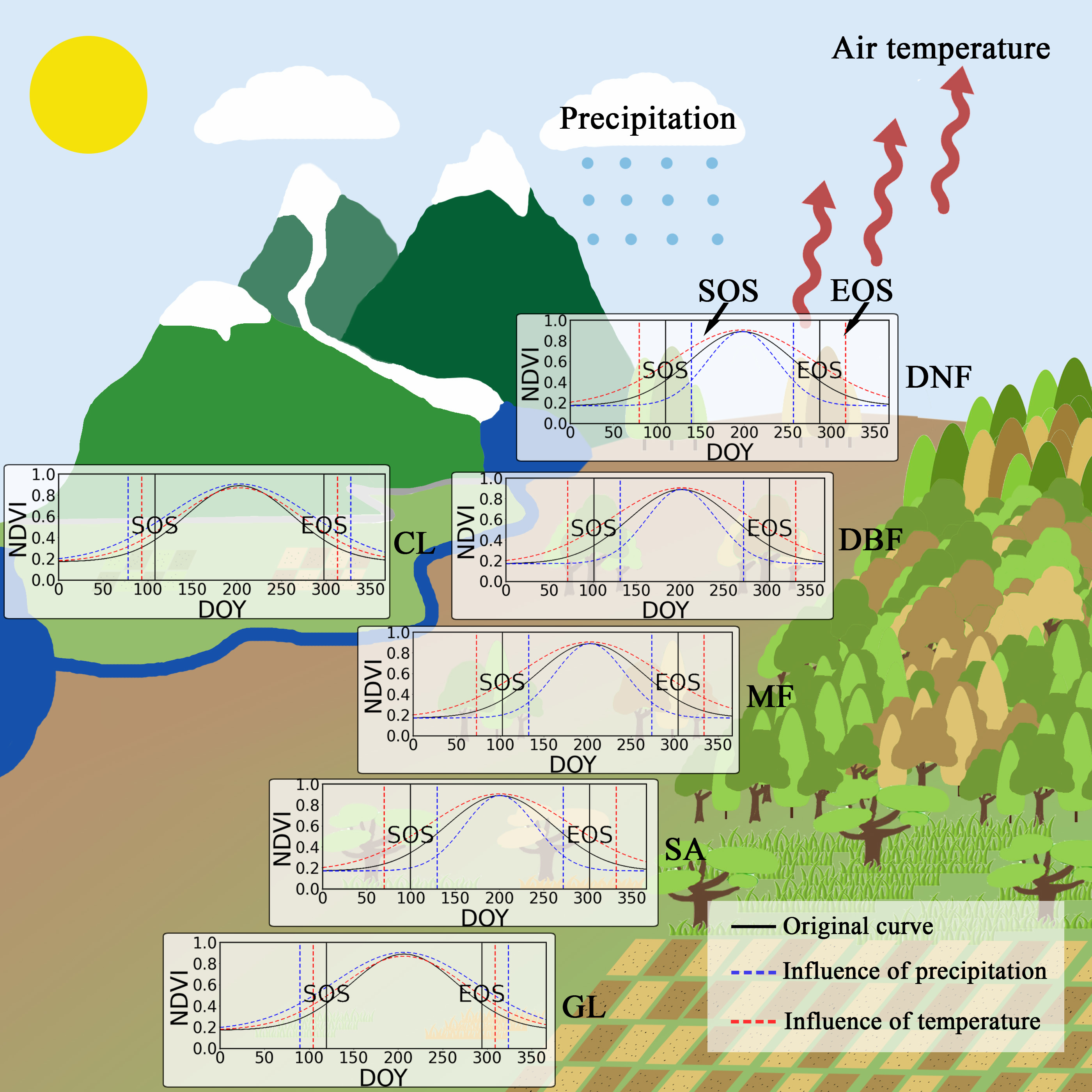
Among the various climate factors, temperature and precipitation prior to the growing season (hereinafter referred to as the “preseason”) play an important role in regulating vegetation phenology. The start date (SOS) and end date (EOS) of the growing season are essential indicators of vegetation phenology. They are directly associated with climatic factors [19]. For example, the plant dormancy period is temperature-controlled vegetation phenology [20]. In regions with a cold season, vegetation must be exposed to sufficient heat accumulation in the growing season in order to break its dormancy and start growing [19]. Therefore, temperature can be considered the most important factor affecting vegetation phenology in many regions [21,22]. Additionally, precipitation is also a key factor that regulates the spring phenology of vegetation in some areas and affects vegetation phenology to a greater extent than the temperature in some areas [23,24,25]. Autumn phenology also plays a prominent role in regulating carbon balance and biomass regionally and globally [26,27]. Studies have shown that temperature has a strong controlling effect on the autumn phenology [28,29]. Higher temperatures tend to delay vegetation EOS [28,30]. However, the effect of temperature on EOS appears to be weaker in the Tibetan Plateau [31]. In the Greater Khingan Mountains, it has also been observed that precipitation, relative to temperature, has a stronger control on EOS [32]. In short, the responses of phenology to preseason temperature and precipitation vary in magnitude and direction, between species and regions, and even between the same species in various regions [33]. These complex response patterns have led to considerable spatial heterogeneity in the relationship between phenology and climate. Although many studies have discussed the relationship between preseason temperature and precipitation and vegetation phenology [24,34,35,36,37,38,39], these conclusions cannot be applied to all regions or all vegetation. Therefore, it is necessary to conduct a comprehensive study on the relationship between vegetation phenology and climatic factors.
In addition, the cultivation methods in China are complex and extremely vulnerable to human activities. This leads to it being more challenging to explore the response patterns of different vegetation types to climate factors, and the complex response patterns of phenology to preseason climate are still unclear for different vegetation types. In the temperate zone north of 30°N in China, vegetation types are abundant and seasonal, and the satellite-derived vegetation index is less affected by solar zenith angle [40]. Compared with south of 30°N in China, the agricultural planting pattern is more simple, with single-season or double-season crops, which is convenient for phenological data extraction. Therefore, we selected the temperate zone north of 30°N in China as the main study area to investigate the relationships between vegetation phenology and preseason temperature and precipitation.
The main purpose of this study is to provide a more macroscopic and comprehensive perspective to explore the response patterns of different vegetation types SOS and EOS to preseason temperature and precipitation. Specifically, we used the GIMMS-NDVI3g (Normalized Vegetation Index for the third generation Global Inventory Monitoring and Modeling System from the AVHRR sensor) dataset to extract vegetation phenology parameters (SOS and EOS) validated by ground observation phenology data. In particular, we considered the phenology of double-cropping crops, which is often ignored in many studies on the relationship between vegetation phenology and climate. Then, we investigated the integrated response of vegetation SOS and EOS to preseason temperature and precipitation from 1982 to 2014. The relationships between the phenology of various vegetation types (including deciduous broadleaf forest, deciduous needle leaf forest, mixed forest, grassland, savanna, wheat, maize, and rice) and climatic factors were also discussed.
2. Materials and Methods
2.1. Study Area
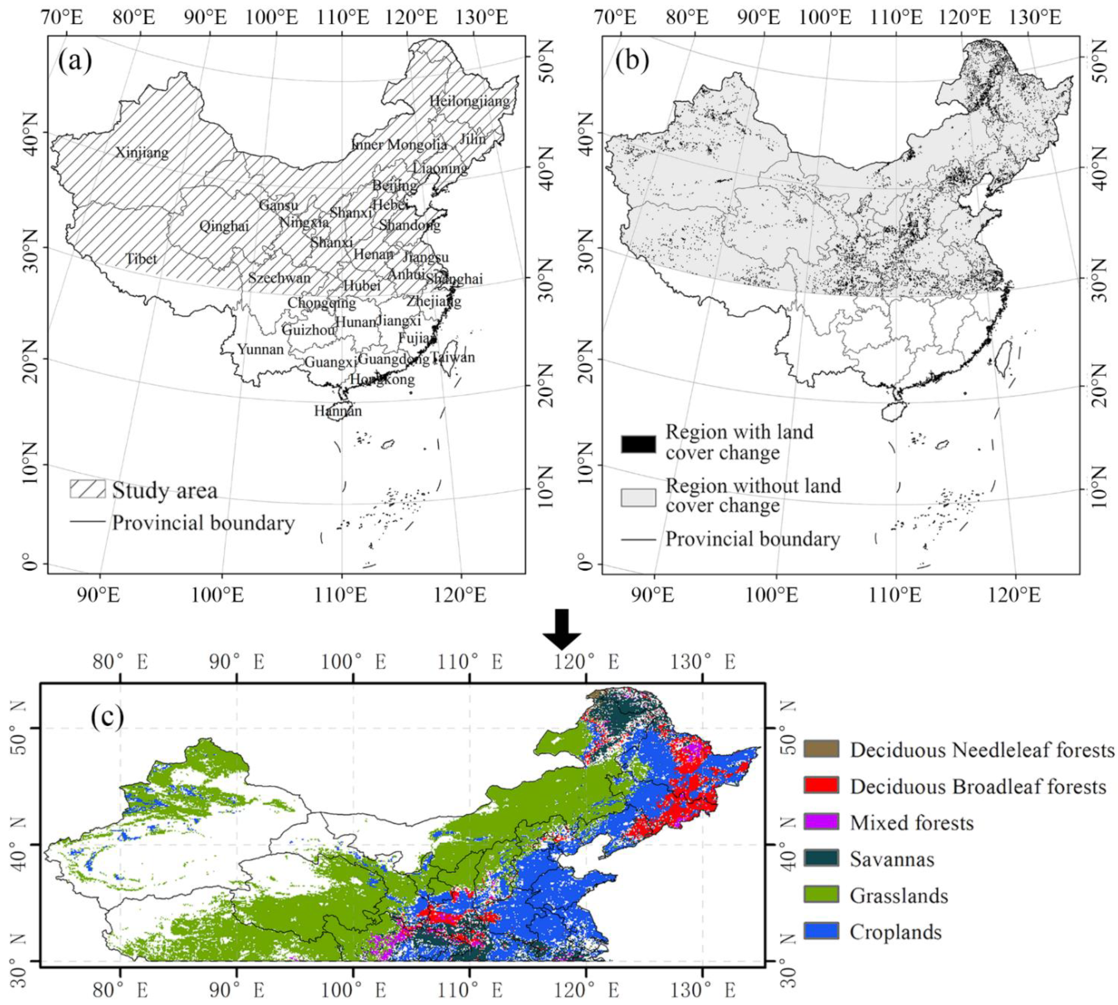
The fluctuations in normalized difference vegetation index (NDVI) are not obvious south of 30°N in China, as a result of the most areas being covered by evergreen forests. In addition, the crops in this area have a complicated planting pattern of three or more seasons a year, which makes it difficult to identify. Therefore, our research focused on the temperate regions of China (north of 30°N; Figure 1a), where the vegetation index retrieved by satellites is also less affected by the solar zenith angle [40]. Considering that the spatial resolution of GIMMS data is 0.08333°, we chose MOD12C1 classification data with a spatial resolution similar to that of GIMMS for the purpose of avoiding the influence of excessive interpolation and resampling on data accuracy. Therefore, based on land use type classification data MCD12C1 (Land Cover Climate Modeling Grid product) from the MODIS (Moderate Resolution Imaging Spectroradiometer) satellite, we excluded the pixels with changes in land use/cover from 2001 to 2014 (data for land use/cover before 2001 were not available) to eliminate errors (Figure 1b). Specifically, we subtracted the 2001 land-use classification data from the 2014 land-use classification data. If the pixel value was equal to 0, this meant that the land use type had remained unchanged, and vice versa. Additionally, non-vegetation land-use types (including Barren, Water Bodies, Urban and Built-up Lands, Permanent Snow and Ice, and Permanent Wetlands) and land-use types of less than 100 pixels were also excluded. Thus, the remaining area in this study was 4.54 million km2 (nearly half of the total land area of China). Vegetation types in the selected study area were classified as listed in Table 1.
2.2. Datasets and Preprocessing
We used the NDVI product of the National Oceanic and Atmospheric Administration (NOAA) Global Inventory Monitoring and Modeling System (GIMMS) to calculate the SOS and EOS (the unit is the number of days in a year) of vegetation from 1982 to 2014. The GIMMS NDVI (version 3g.v1) dataset, which has a spatial resolution of 0.0833333° and a temporal resolution of twice a month, can be downloaded from https://iridl.ldeo.columbia.edu/SOURCES (accessed on 19 January 2021).
The ground-based data for crops were derived from the 10-day value dataset of crop growth of China Meteorological Data Network (http://data.cma.cn/ (accessed on 23 January 2021)). It contains information on the development period, plant height, soil moisture, etc., of different crops, observed at 778 sites from 1992 to 2013 and is widely used in Crop Phenology research [41,42]. We finally selected crop growth records of wheat, corn, and rice at 671 sites from 1992 to 2013 (some sites do not contain phenological information of the required crop types). The turning-green period of maize, the emergence period of wheat, and the transplanting period of rice in the ground-based dataset were defined as SOS, and the maturity period of maize, wheat, and rice in the ground-based dataset corresponded to EOS [43]. The meteorological data covering 33 years (1982–2014) of daily precipitation and temperature from 786 monitoring stations were derived from the China Meteorological Data Network (CMDN) (http://data.cma.cn/ (accessed on 18 January 2021)). We used the spline interpolation method to generate raster data with a spatial resolution of 0.83333° to match the phenological data in the study area [44].
MCD12C1 datasets contain 3 sets of land use classification schemes, among which the IGBP (International Geosphere Biosphere Program Version 6) classification scheme has been widely used in various vegetation studies [45,46,47]. Therefore, we used the IGBP (International Geosphere Biosphere Program Version 6) classification data from MODIS MCD12C1 in 2001 and 2014 for vegetation classification. The original data, with a spatial resolution of 0.05°, were resampled to generate a new dataset with a resolution of 0.83333° (with the nearest neighbor method). In addition, the IGBP classification system divides land-use types into 17 categories, including land-use types without vegetation cover. Therefore, according to the research needs of this study, we eliminated the following pixels:
- Pixels that showed changes in land-use type between 2001 and 2014;
- Minor vegetation types (less than 100 pixels) in the study area;
- Non-vegetated land-use types, such as bare land and urban built-up areas.
2.3. Calculation and Validation of Phenological Data
We used the Savizky–Golay (SG) filter to reconstruct the NDVI time series curve for each pixel. The SG filter can retain data information to the greatest extent while removing data noise, and it is more suitable for extracting double-season crop information [48]. The formula of SG filtering is given as:
where and are the th value of the filtered data and the original data, respectively, is the th weight value of the filtering window and is calculated by polynomial fitting with the polynomial order of 4, and m is half the size of the filtering window (=6). Finally, a quadratic spline was used to interpolate the data to daily values [49].
After reconstructing the NDVI time series curve, we selected pixels with one or two maxima (the pixels with two maxima were the candidates for double-season crops) and calculated the second derivative. Two local maximum (inflexion) points in the first half of growth season were regarded as the SOS and the second half as the EOS [50]. To extract the phenological parameters of different crops accurately, we determined the limited time window to be 30 days before and after the average value of the phenological parameters (SOS and EOS) of various crops in different provinces based on ground-measured phenological data [43]. If the estimated SOS and EOS meet the restricted time window of a certain crop (i.e., maize, wheat, and rice), then the corresponding pixel is associated with the crop. If the SOS and EOS of the pixel with a double-season crop meet the limited time windows of both crops, then the pixel is associated with a double-season crop.
Finally, we used ground-based phenological dates to validate calculated phenological dates for wheat, corn, and rice from 1992 to 2013. Four statistics were used to verify the calculated phenological dates, including Nash coefficient of determination (R2) [51], normalized root means square error (NRMSE) [52], Nash–Sutcliffe efficiency (NSE) [53], and percentage bias (PBIAS) [54].
where and are the predicted phenological sequence data and their mean values, and and are the phenological series data and their mean values observed on the ground.
2.4. Statistical Analysis
The Theil–Sen (TS) method was used to estimate the long-term trend in EOS/SOS for each pixel from 1982 to 2014 [55,56]. It is a robust method for monitoring trends in time series and is only slightly affected by outliers [57]. The Mann–Kendall (MK) method was used to test the significance of the long-term trend in EOS/SOS [58,59]. The TS and MK methods have been widely used in detecting long-term phenological trends [60,61] and have been shown to exhibit strong stability [57,62,63,64].
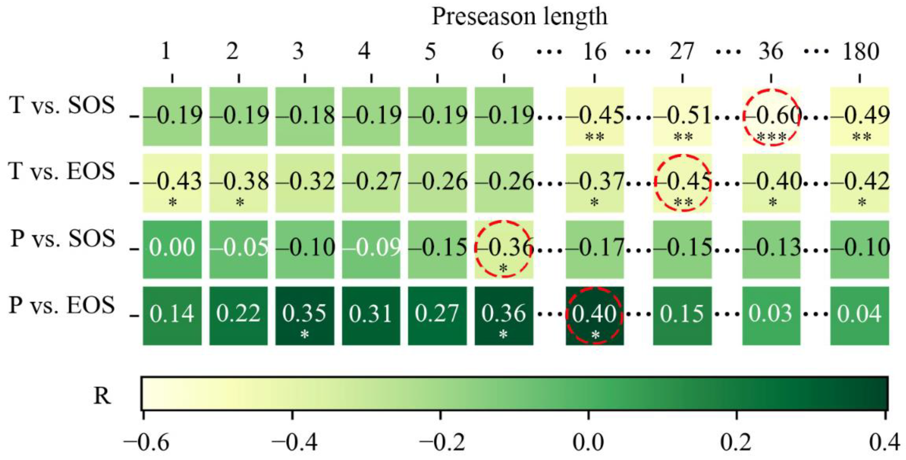
To explore the lag effects of temperature and precipitation on vegetation phenology, we further calculated preseason lengths (in days) for SOS and EOS in each pixel. Here, the preseason length is defined as the n days before the 33-year average SOS/EOS dates for each pixel (1 ≤ n ≤ 180) (similar to “time window durations” discussed in Ren, Li, and Peichl [22]). Preseason temperature and precipitation are the average daily temperature and precipitation for different preseason lengths [65]. We used the partial correlation analysis and T-test to investigate the correlation between SOS/EOS and the preseason precipitation/temperature at each pixel for different preseason lengths (1–180 days). As a result, we obtained 4 × 180 partial correlation coefficients per pixel (Figure 2). Finally, the preseason length of the highest absolute value of the partial correlation coefficient was selected as the optimal time scale of each category (similar to “best-performing time window durations” in [22]). For example, as shown in Figure 2, the highest partial correlation coefficient between the preseason temperature and SOS of the pixel in row i and column j is −0.60. Therefore, −0.60 was defined as the final partial correlation coefficient between the preseason temperature of the pixel and SOS, and the corresponding preseason length 36 was the optimal time scale between the preseason temperature and SOS in this pixel. Finally, we analyzed the partial correlation between EOS/SOS and preseason temperature/precipitation for each vegetation type from 1982 to 2014 to further study the response patterns of SOS and EOS of the various vegetation types to preseason temperature and precipitation.
3. Results
3.1. Validation of Phenological Data and Its Long-Term Trend
3.1.1. Validation of Satellite-Based Phenology Data
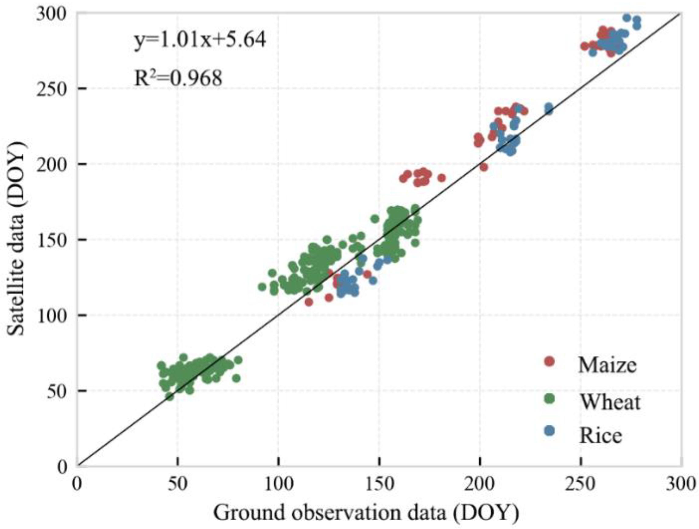
The phenological dates of ground observations for crops from 1992 to 2013 were compared to the NDVI-based dates. The verification results were shown in Figure 3 and Table 2. The crop phenology data were in good agreement with the ground observation data, with R2 of 0.968, NRMSE of 10.2%, and PBIAS of −5.3%. The R2 of three crop types (wheat, maize, and rice) were all ≥0.97. Except for wheat (the NRMSE equals 11.540), the NRMSE of the other two crops were all <10%. In general, the extracted phenology data met the data accuracy requirements.
3.1.2. Long-Term Change in Vegetation Phenology
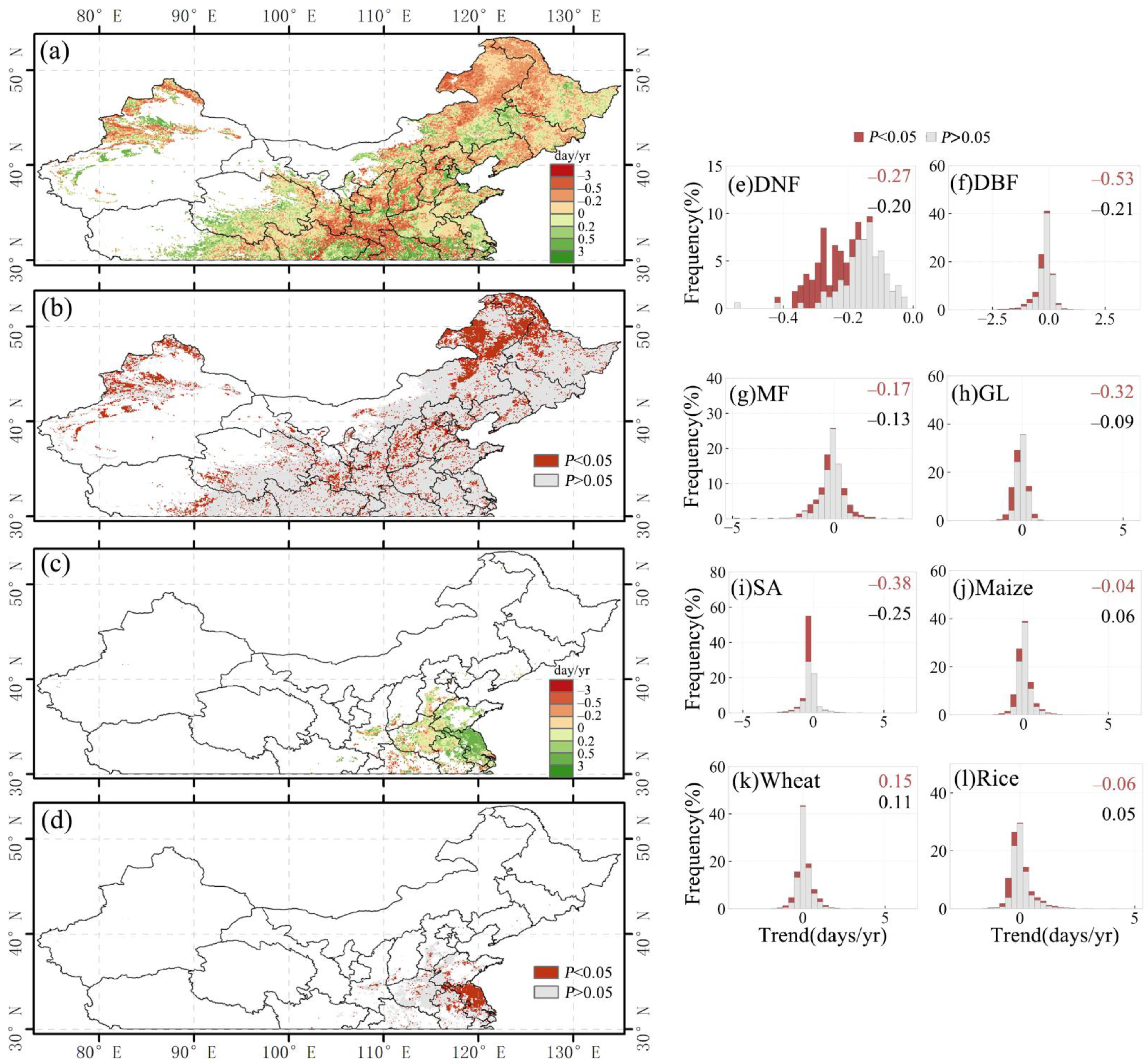
There was an overall advanced SOS trend for a large portion of pixels from 1982 to 2014 over the whole study area (Figure 4a,c). A total of 19.3% of the study area (about 875,766 km2) had a significant change of SOS from 1982 to 2014 (p-value < 0.05), of which 13.5% (about 612,446 km2) showed an advanced trend and 5.8% showed a delayed trend. On average, the SOS within this 19.3% of the study area was advanced by 0.15 days/yr from 1982 to 2014 (Figure 4a,c). The spatial distribution shows that the delayed SOS was relatively scattered over the study area, while advanced SOS was relatively concentrated at the intersection of the Inner Mongolia Autonomous Region and Jilin Province of Northeast China (Figure 1a vs. Figure 4a,c). The SOS of deciduous broadleaf forest and savanna have the largest advanced days, about 0.53 days/yr and 0.38 days/yr, respectively (p-value < 0.05), while the SOS of maize and rice have the smallest advanced days, with values of 0.04 days/yr and 0.06 days/yr, respectively (p-value < 0.05) (Figure 4e–l).
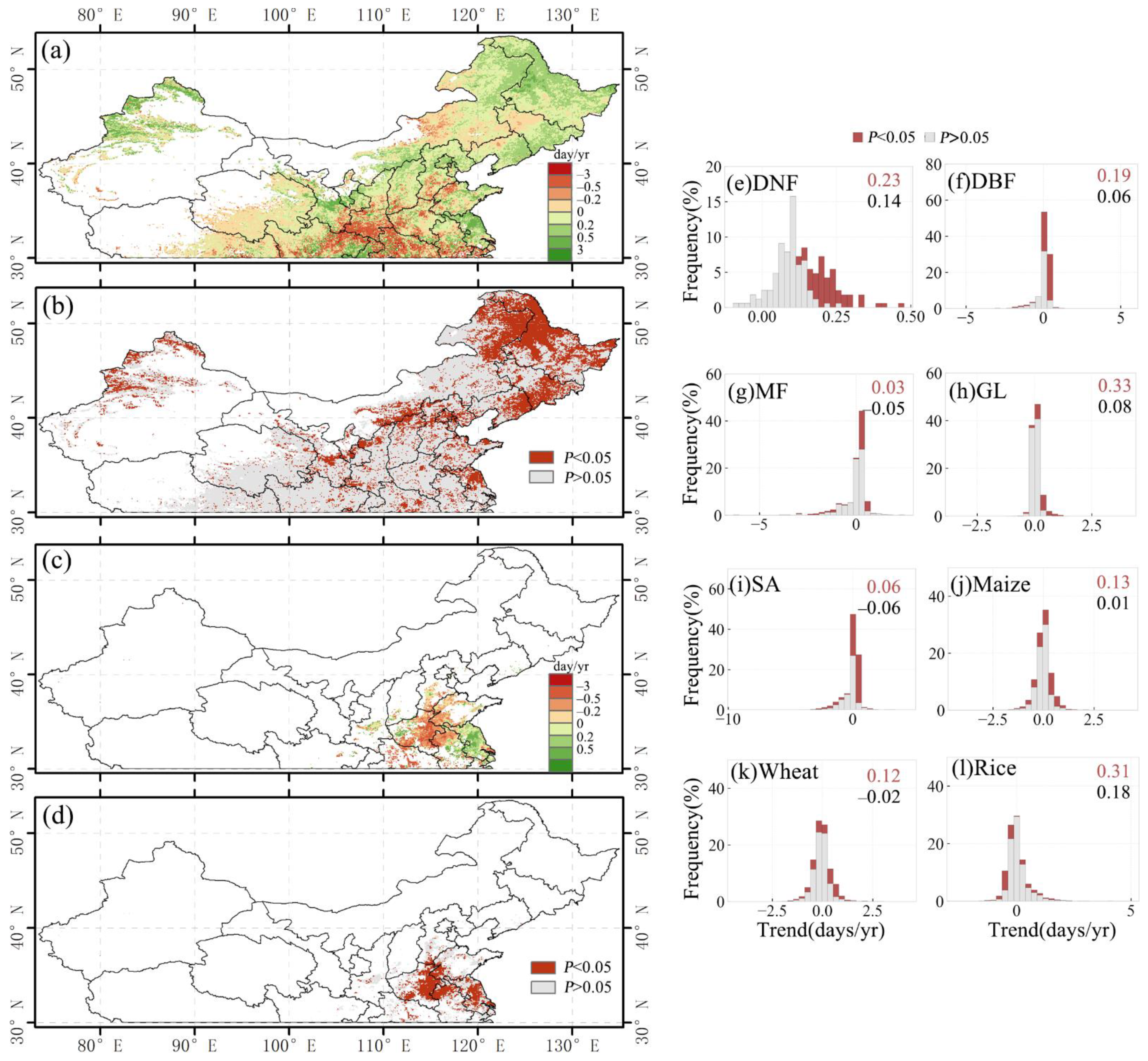
As for the EOS, there was an overall delayed trend for a large portion of the study area (Figure 5a,c). There was a significant change of EOS in 27.5% (about 1.25 million km2) of the study area (p-value < 0.05), of which 23.1% (about 1.05 million km2) showed a significantly delayed trend and only 4.4% (about 201,122 km2) showed a significant advanced trend. Overall, EOS was delayed by 0.19 days/yr in 27.5% of the study area. Compared with SOS, the geographical distribution of EOS with a significant delay trend was more concentrated for savanna in the northeast and cropland in the east (Figure 1a vs. Figure 5a,c). The EOS of grassland and rice had the largest number of days’ delay, about 0.33 days/yr and 0.31 days/yr, respectively (p-value < 0.05), while the EOS of savanna and mixed forest had the smallest number of days’ delay, with values of 0.06 days/yr and 0.03 days/yr, respectively (p-value < 0.05) (Figure 5e–l).
3.2. Relationship between SOS and Preseason Temperature and Precipitation
3.2.1. Overall SOS Response and Spatial Distribution
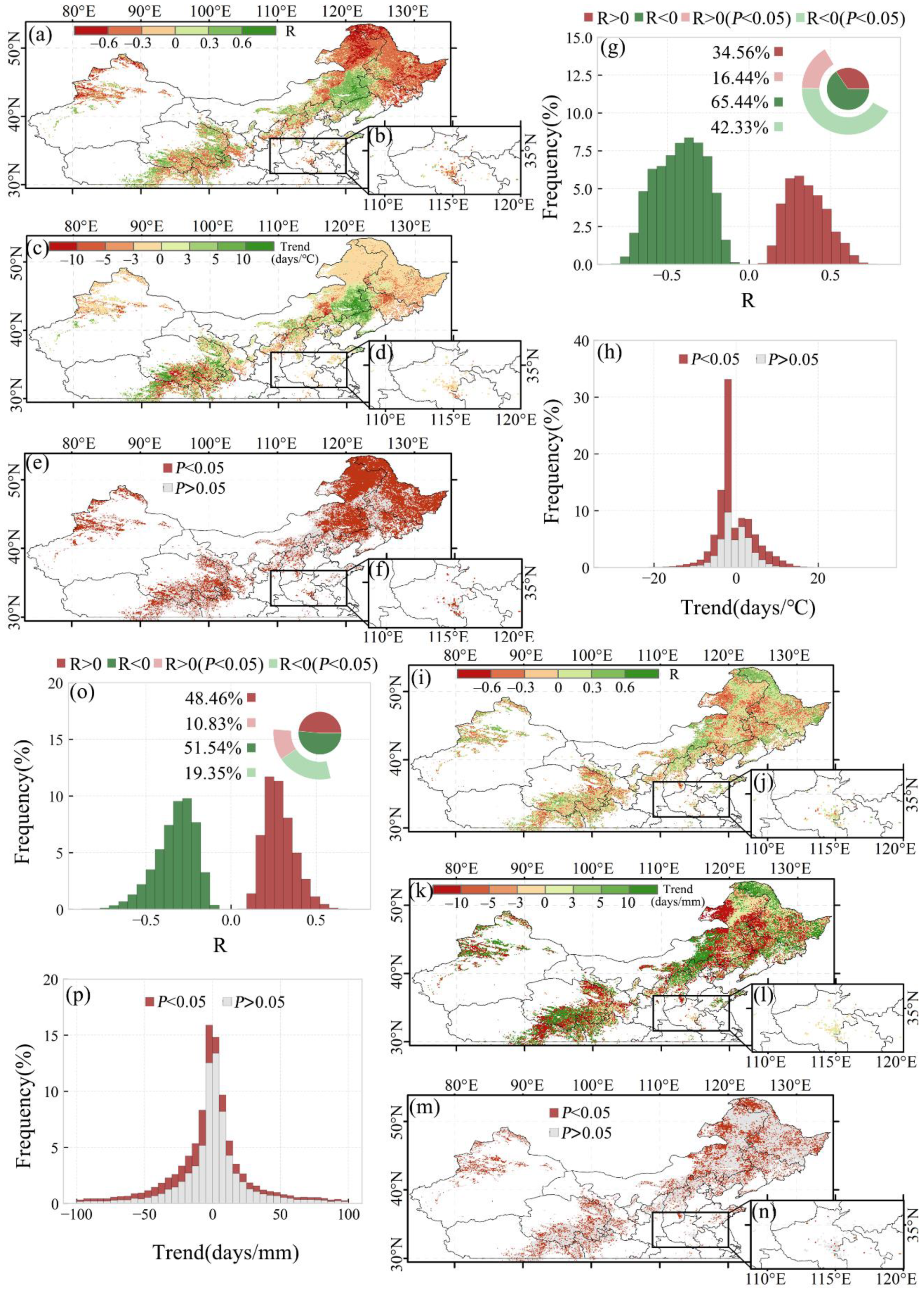
Spatial distribution of the correlations between SOS and preseason temperature for the first and second season of the double-season crop as well as single-season vegetation are shown in Figure 6a,b. The SOS changing rate per preseason temperature and the significance level of the correlations are shown in Figure 6c–f. We found that about 65.4% (approximately 1.57 million km2) of the study area showed a negative correlation between SOS and preseason temperature, with 42.3% (about 1.02 million km2) having a significant negative correlation (p-value < 0.05, Figure 6g). About 16.4% (about 395,443 km2) of the study area had a significant positive correlation (p-value < 0.05; Figure 6g). For every 1 °C increased in preseason daily mean temperature at the optimal time scale, the SOS advanced 0.62 days (p-value < 0.05) (Figure 6h).
Spatial distribution of the correlations between SOS and preseason precipitation for the first and second season of the double-season crop as well as single-season vegetation are shown in Figure 6i,j. The SOS changing rate per preseason precipitation and the significance level of the correlations are also shown in Figure 6k–n. The relationship between vegetation SOS and preseason precipitation was not as significant as the preseason temperature for the study area. We found that the SOS was negatively correlated with preseason precipitation (p-value < 0.05) in 19.4% (about 465,440 km2) of the study area, whereas the area in which SOS was positively correlated with preseason precipitation was only 10.8% (about 260,502 km2) (p-value < 0.05) (Figure 6o). Apparently, preseason temperature and precipitation showed varying degrees of influence on SOS in the study area. Although the influence of preseason precipitation on SOS was not obvious, preseason precipitation explained variations in the SOS for areas where preseason temperature could not, such as the border area between Inner Mongolia and Liaoning Province (Figure 6e,m).
3.2.2. SOS Responses of Different Vegetation Types
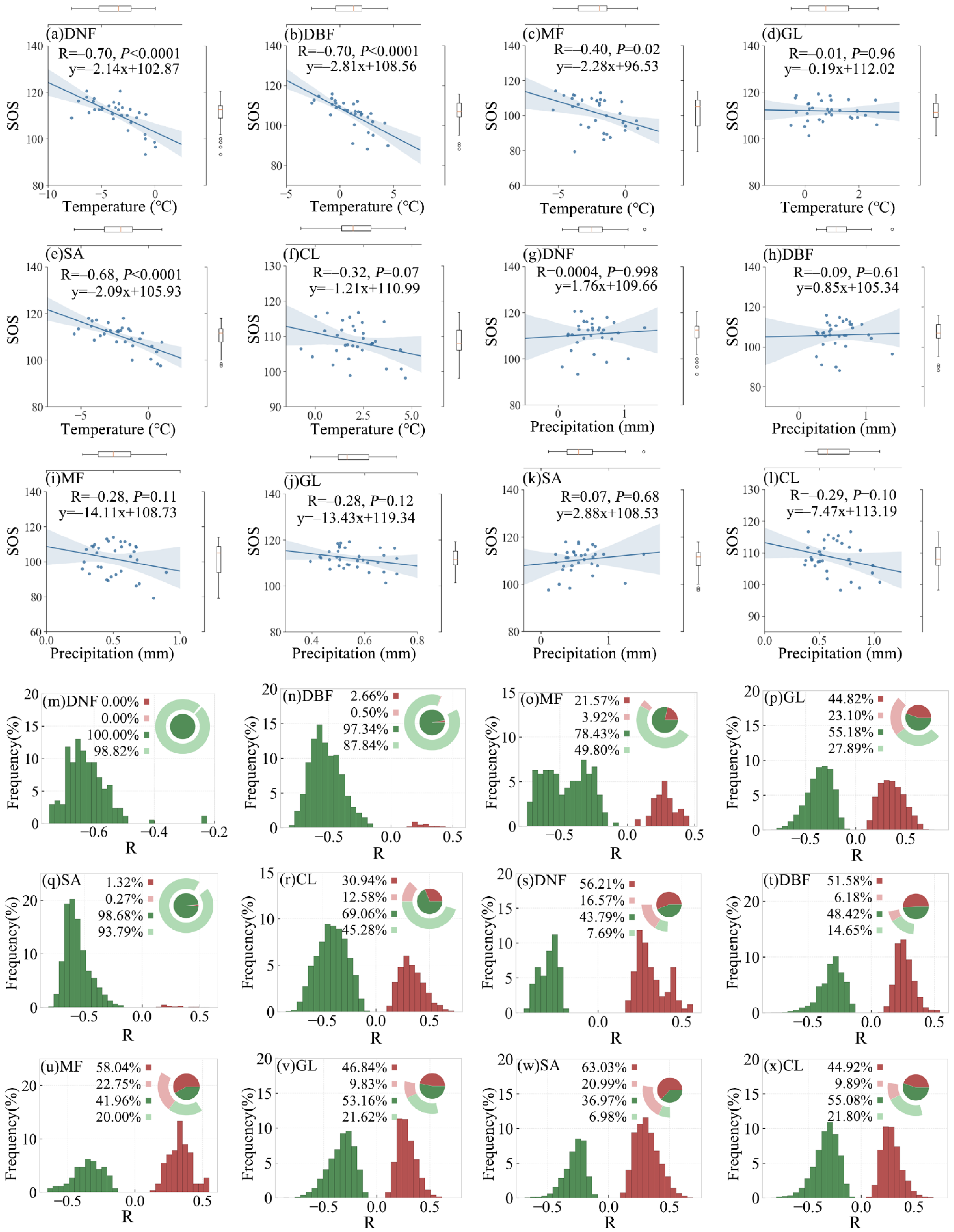
The partial correlation between preseason temperature/precipitation and SOS for the six vegetation types in the study area is shown in Figure 7a–l. The partial correlation coefficient between preseason temperature and SOS were mostly negative (ranging from −0.01 to −0.70), indicating similar response patterns for the six vegetation types. Among the six vegetation types, the partial correlations were stronger for the deciduous broadleaf forest, deciduous needle leaf forest, mixed forest, and savanna, with R values of ≤−0.40 (p-value < 0.05), while for grassland and cropland, the partial correlations were relatively weaker, with R values of −0.01 and −0.32, respectively. We found that the SOS advanced for more than 2 days for every 1 °C increase in preseason temperature for deciduous needle leaf forest, deciduous broadleaf forest, mixed forest, and savanna, indicating higher sensitivity. However, there was no significant partial correlation between the preseason precipitation and the SOS of each vegetation type.
The frequency distribution of partial correlation coefficients between preseason temperature/precipitation and SOS for the six vegetation types is shown in Figure 7m–x. For deciduous needle leaf forest, deciduous broadleaf forest, mixed forest, and savanna, partial correlation coefficients between preseason temperature and SOS were mostly negative (98.8%, 87.8%, 49.8%, and 93.8%, respectively; p-value < 0.05). The effect of temperature on vegetation spring phenology is stronger than that of precipitation on vegetation spring phenology.
3.3. Relationship between EOS and Preseason Temperature and Precipitation
3.3.1. Overall EOS Response and Spatial Distribution
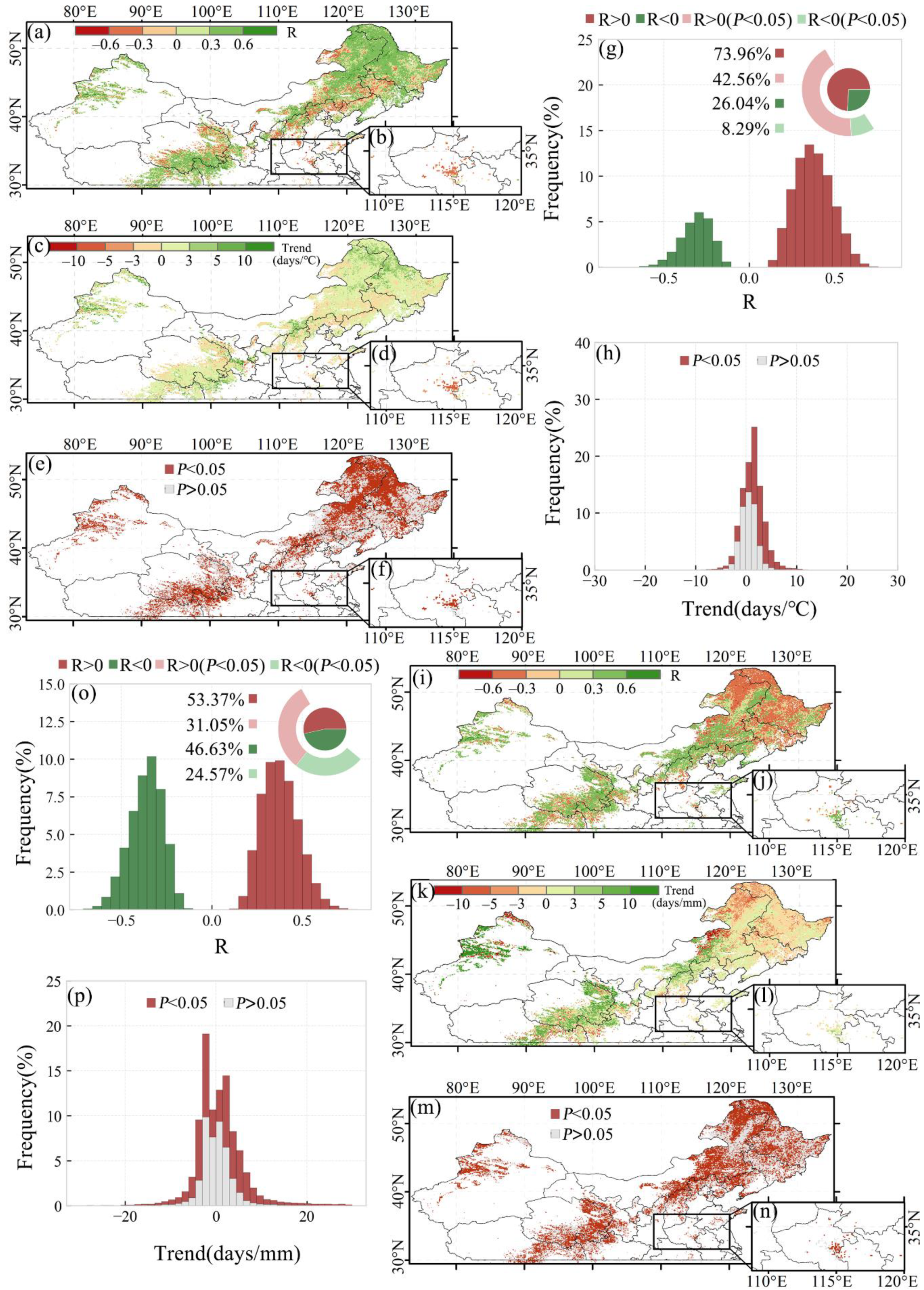
Spatial distribution of the correlations between EOS and preseason temperature for the first and second season of the double-season crop as well as single-season vegetation are shown in Figure 8a,b. The EOS changing rate per preseason temperature and the significance level of the correlations are also shown in Figure 8c–f. The response of vegetation EOS to preseason temperature was overall opposite to that of SOS. About 74.0% (about 1.78 million km2) of the study area showed a positive correlation between EOS and preseason temperature, with the remaining 26.0% (about 626,360 km2) of the study area showing a negative correlation. Among them, 42.6% (about 1.02 million km2) of the area showed a significant positive correlation between EOS and preseason temperature (p-value < 0.05), whereas only 8.3% (about 199,405 km2) of the area showed a significant negative correlation between EOS and preseason temperature (p-value < 0.05) (Figure 8g). For each 1 °C increase in the preseason daily mean temperature in the optimal time scale, the appearance of EOS was estimated to be delayed by 2.01 days (Figure 8h).
Spatial distribution of the correlations between EOS and preseason precipitation for the first and second season of the double-season crop as well as single-season vegetation are shown in Figure 8i,j. The EOS changing rate per preseason precipitation and the significance level of the correlations are also shown in Figure 8k–n. For preseason precipitation, about 55.6% (about 1.34 million km2) of the study area showed a significant correlation with EOS (p-value < 0.05). Of this, about 31.1% and 24.6% of the study area showed a significant positive and negative correlation, respectively, between EOS and preseason precipitation (Figure 8o). On average, an increase in daily mean precipitation of 1 mm in the optimal time scale caused a delay in EOS by 1.86 days (Figure 8p). In general, vegetation EOS in most of the area has a significant positive correlation with preseason temperature, while the correlation with preseason precipitation is subtle. However, preseason precipitation can explain changes in EOS that cannot be explained by preseason temperature in some regions, such as the border area of Inner Mongolia and Heilongjiang Province reflecting the complex internal impact mechanism of preseason precipitation on EOS (Figure 8e,m).
3.3.2. EOS Responses of Different Vegetation Types
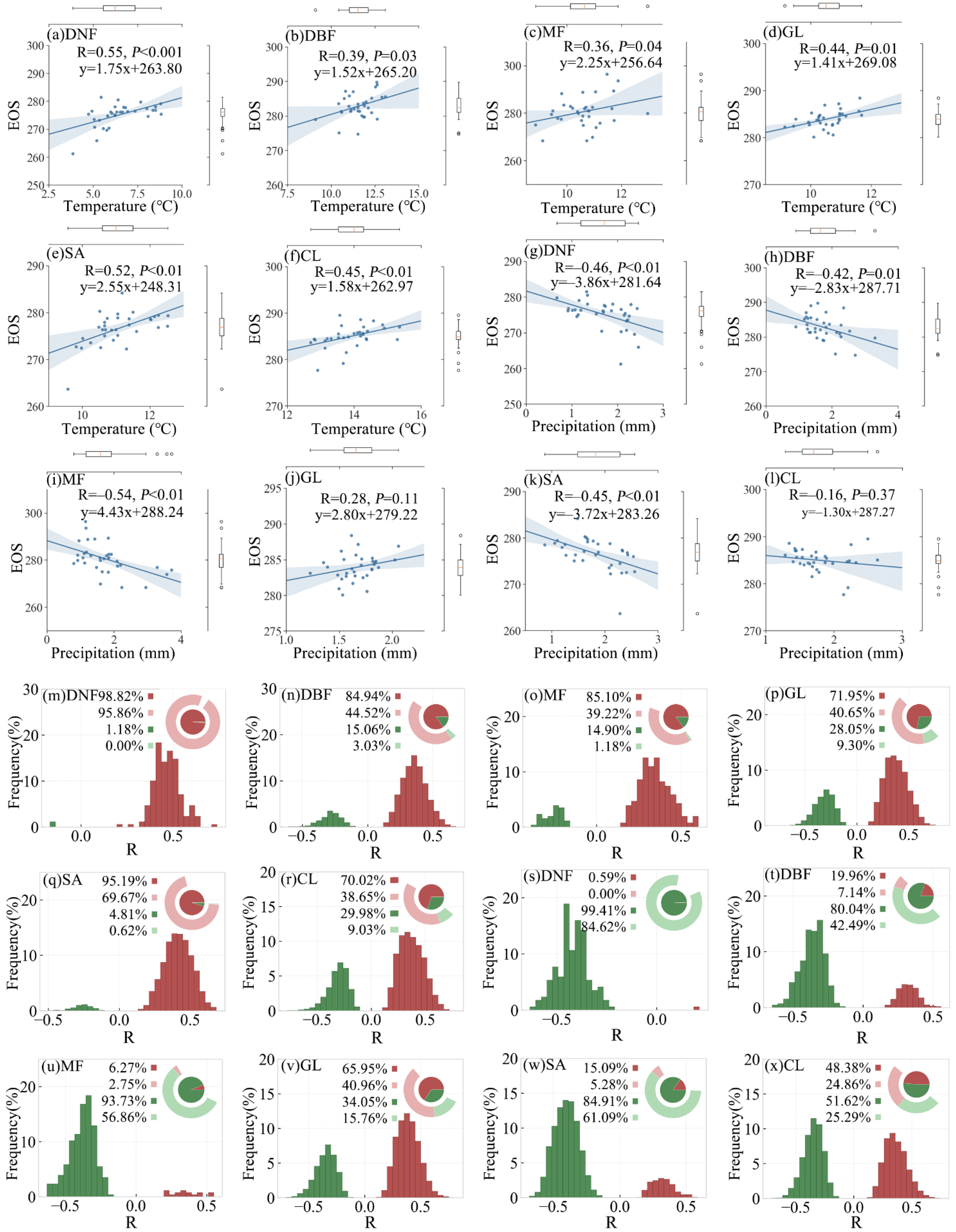
The partial correlation between preseason temperature/precipitation and EOS for the six vegetation types in the study area is shown in Figure 9a–l. In contrast with the response pattern of the SOS to preseason temperature, the partial correlations between preseason temperature and EOS were mostly positive (ranging from 0.36 to 0.55; Figure 9g–l). Greater correlation coefficients were found for deciduous needle leaf forest and savanna (0.55 and 0.52, respectively; p-value < 0.05). The EOS for mixed forest and savanna showed greater sensitivity to preseason temperature, with more than 2 days delay per 1 °C increased (Figure 9g,k). As opposed to the response pattern of the SOS/EOS to preseason temperature, the partial correlation between preseason precipitation and EOS was inconsistent across various vegetation types. For example, partial correlation coefficients between preseason precipitation and EOS were mostly negative for deciduous needle leaf forest, deciduous broadleaf forest, mixed forest, and savanna (−0.46, −0.42, −0.54, and −0.45, respectively; p-value < 0.05), which was opposite to the partial correlation pattern between preseason temperature and EOS. Among them, the EOS of the mixed forest was the most sensitive to preseason precipitation, with more than 4 days’ delay per 1 mm increase in precipitation.
The frequency distribution of correlation coefficients between preseason temperature/precipitation and EOS for the six vegetation types is shown in Figure 9m–x. For deciduous needle leaf forest, deciduous broadleaf forest, mixed forest, and savanna, the partial correlation coefficients between EOS and preseason temperature were mostly positive (95.9%, 44.5%, 39.2%, and 69.7%, respectively; p-value < 0.05), while the partial correlation coefficients between EOS and preseason precipitation were mostly negative (84.6%, 42.5%, 56.9%, and 61.1%; p-value < 0.05). For grassland, the partial correlation coefficients between preseason precipitation and SOS were mainly negative (with the proportion of 21.6%), whereas the partial correlation coefficients with EOS were mainly positive (with the proportion of 41.0%). The partial correlations between preseason precipitation and EOS for grassland and cropland were not as significant as for the other vegetation types.
3.4. Optimal Time Scale for Preseason Temperature and Precipitation
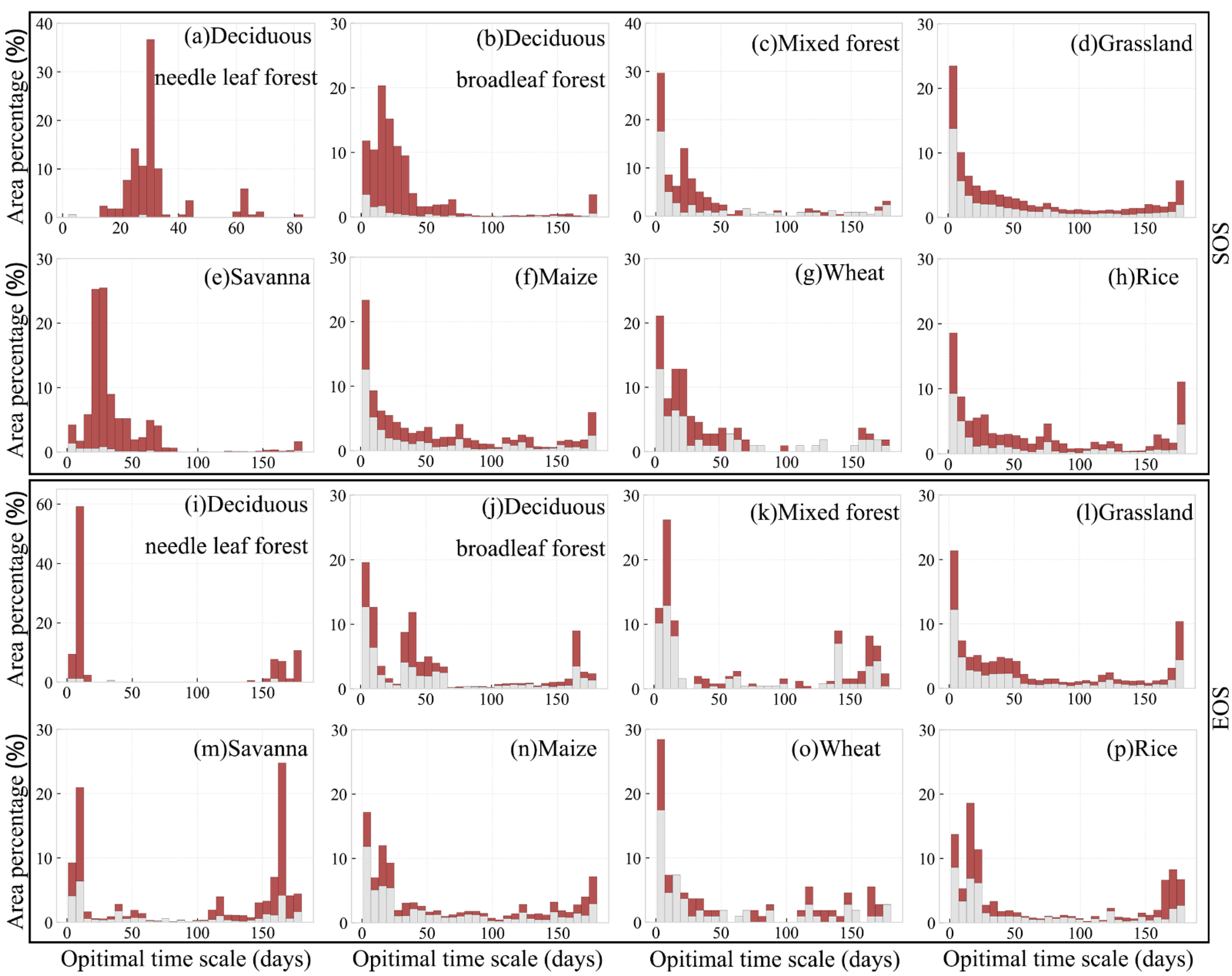
Area percentage distribution of optimal time scale for preseason temperature and precipitation impacts on SOS for different vegetation types are shown in Figure 10. In general, the preseason length where the temperature had the greatest influence on SOS was mainly concentrated at the range of 0–60 days. The optimal time scales for deciduous needle leaf forest, deciduous broadleaf forest, and savanna were mostly concentrated in 20–40 days (79.3%; p-value < 0.05), 0–50 days (75.1%; p-value < 0.05), and 0–75 days (90.0%; p-value<0.05), respectively. Please note that, as the preseason length increased, the influence of preseason temperature on the SOS gradually diminished. In contrast, the distribution of optimal time scale for the influence of preseason temperature on vegetation EOS was more scattered. For example, although the optimal time scale of most pixels was concentrated in 0–30 days, there are still about 17.8% (deciduous needle leaf forest), 8.4% (deciduous broadleaf forest), 9.8% (mixed forest), 6.6% (grassland), 33.0% (savanna), 9.2% (maize), 6.4% (wheat), and 17.7% (rice) of pixels with the optimal time scale concentrated in 150–180 days (p-value < 0.05). Therefore, preseason temperature showed a more profound impact on autumn vegetation phenology of vegetation in the study area.
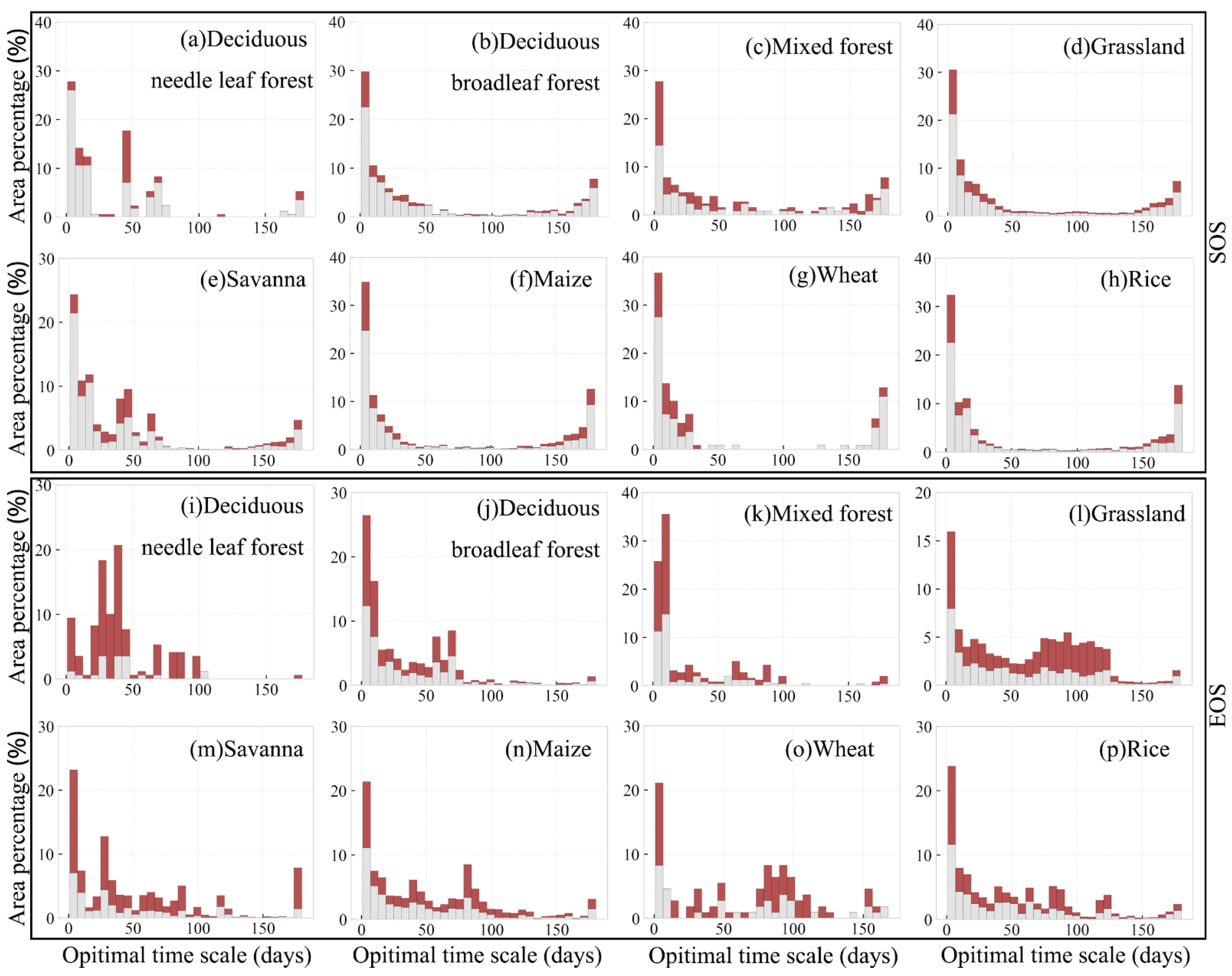
Area percentage distributions of optimal time scale for preseason temperature and precipitation impacts on EOS for different vegetation types are shown in Figure 11. Although the optimal time scale pixels were mostly concentrated in 0–30 days, their distributions were not concentrated for the SOS (Figure 11a–h), showing that the impact of precipitation on vegetation SOS was not as significant as temperature. In contrast, the impact of precipitation on vegetation EOS was stronger than the impact on SOS. The optimal time scale was also concentrated in 0–60 days. At the same time, the rainfall in the 60–100 days of many pixel seasons also had a strong control effect on the vegetation EOS. The impact of preseason precipitation on EOS gradually diminished as the preseason time increased (Figure 11i–p).
4. Discussion
4.1. Effects of Preseason Temperature on Vegetation Phenology
In most temperate regions of China, we observed a significant negative correlation between the spring phenology of vegetation and preseason temperature, as well as a significant positive correlation between autumn phenology and preseason temperature (Figure 6 and Figure 8), which is consistent with observations of a previous study [25]. The results suggest that higher temperatures will advance SOS and delay EOS in most temperate regions of China. Sufficient heat accumulation is required for the onset of vegetation growth [66]. Generally, the temperature in the study area needs to reach 0–5 °C in order to end the dormant period and meet the necessary weather conditions for leaf onset [19]. Higher temperatures can accelerate heat accumulation, thereby promoting the greening of vegetation. This is why the optimal time scale of the preseason temperature was concentrated in the 0–60 days prior to the mean SOS, which is also known as the dormant period.
Preseason temperature also has a significant controlling effect on autumn phenology (Figure 8). According to reports, higher temperatures in summer and autumn will increase the activity of photosynthetic enzymes and reduce the degradation rate of chlorophyll, leading to the delay of EOS [32,67]. At the same time, higher preseason temperature is also a sign of warm winter, which means that extreme weather conditions such as frost are less harmful to vegetation [68]. In short, the senescence of vegetation is a complex and slow process involving many non-biological factors [69,70], which are beyond the scope of this article, except for preseason temperature and precipitation.
Although the optimal time scale of temperature for the EOS was mainly concentrated at 0–60 days in the study area, there were also many areas where the optimal time scale of temperature was concentrated at 120–180 days. This may be attributed to the fact that a higher temperature in spring would quickly lead to the accumulation of the heat required for vegetation growth, giving rise to the rapid growth of vegetation and promoting the early start of autumn phenology [66]. In addition, the correlation between the SOS of vegetation (grassland and cropland) and preseason temperature was weaker than that for the other four vegetation types, as has also been reported in other studies [71].
4.2. Effects of Preseason Precipitation on Vegetation Phenology
Compared with temperature, the responses of vegetation phenology to preseason precipitation in temperate regions of China were more complex. For deciduous needle leaf forest, deciduous broadleaf forest, mixed forest, and savanna, the correlations between preseason precipitation and SOS were not significant. This may be due to the well-developed root system of the woodland, the stronger soil water storage capacity, and therefore the stronger resistance to drought [34]. Furthermore, temperate forests have relatively low evapotranspiration and high precipitation. They can retain water for the next rainy season, which reduces the impact of drought on vegetation [72]. Therefore, the change of preseason precipitation has a minor influence on the spring phenology of forests.
Interestingly, we found that the EOS of deciduous coniferous forest, deciduous broad-leaved forest, mixed forest, and savanna were mainly negatively correlated with preseason precipitation. This may be related to the average precipitation in the region [71]. Excessive precipitation may cause the vegetation growing season to end prematurely in areas with abundant precipitation. Studies have shown that soil moisture affects the growth of vegetation [73,74,75,76,77]. The increase in soil moisture may promote the photosynthesis of vegetation, which in turn prompts the early end of the vegetation growing season [32,78]. Other climatic factors, such as snowmelt, may also replenish soil moisture, leading to an earlier fall of vegetation phenology. In addition, due to the influence of permafrost in some forests in cold regions, high soil moisture can easily limit the absorption of soil nutrients by vegetation, thereby ending growth prematurely [32,79].
The impact of precipitation on vegetation EOS was greater than that on vegetation SOS. For many vegetation types, the effect of precipitation on EOS was stronger and more complex than that of temperature. The responses of vegetation phenology to precipitation in various vegetation types and regions are different. Excessive rainfall surplus or deficit can affect vegetation growth. In short, vegetation senescence is a complicated process and the understanding of its relationship with climatic factors needs to be further investigated in detail. There is no dispute that temperature has a strong control on EOS. However, the effect of precipitation on vegetation phenology is more complex and is related to multiple other factors. Therefore, the influence of extreme conditions and composite factors should be further considered in future research on the relationship between vegetation phenology and precipitation.
4.3. Impacts, Limitations, and Future Work
This study showed that vegetation phenology was significantly correlated with preseason temperature and preseason precipitation. Generally, there was a negative correlation between temperature and vegetation SOS, and a positive correlation between temperature and vegetation EOS in the temperate regions of China. The effect of precipitation on vegetation phenology was much more complicated, with various patterns of influence depending on the region and vegetation type. Overall, this study comprehensively explored the relationship between SOS/EOS of different vegetation types and preseason temperature/precipitation, therefore contributing to the study of the complex influencing mechanisms between vegetation phenology and climate.
Our study focused on the different response patterns between various vegetation types. However, many studies have shown that phenology of the same vegetation type may respond differently to climatic factors depending on other factors such as geographical conditions [21]. This topic will be considered in future work. In addition, owing to limitations in spatial resolution of used datasets, we only limited our study to five natural vegetation types and three crops. With the help of higher-spatial-resolution data, it will be necessary in future to explore the phenology variations of more vegetation types in response to preseason temperature and precipitation.
5. Conclusions
In this study, we investigated long-term phenological trends in the mid-latitude region of China from 1982 to 2014. In particular, we analyzed the SOS/EOS response patterns of various vegetation types to preseason temperature and preseason precipitation. The preseason length of optimal influence was also examined. Moreover, the complex interaction mechanisms between vegetation phenology and climate were explored.
The results show that the SOS of vegetation in most regions within the study area had an advanced trend, whereas the EOS had a delayed trend from 1982 to 2014. The phenology of various vegetation types had the same response pattern to preseason temperature, which exerted a strong controlling effect. In contrast, the phenology of various vegetation types had different response patterns to preseason precipitation, which showed a stronger effect on EOS than on SOS in many areas. The impact of precipitation on vegetation types was relatively more complex.
In summary, this article presents a comprehensive analysis of SOS/EOS response patterns of various vegetation types to preseason temperature and preseason precipitation in the mid-latitude region of China from 1982 to 2014. We have discussed the influence of water and heat conditions on vegetation phenology and further revealed the relationship between vegetation phenology and climate factors.
Author Contributions
R.Z.: Conceptualization, Formal analysis, Software, Investigation, Writing—original draft. J.Q. and S.L.: Writing—review & editing. Q.W.: Conceptualization, Methodology, Project administration, Validation, Supervision, Funding acquisition. All authors have read and agreed to the published version of the manuscript.
Funding
This research was funded by the Natural Science Foundation of Fujian Province (2021J01627) and the National Natural Science Foundation of China (41601562).
Institutional Review Board Statement
Not applicable.
Informed Consent Statement
Not applicable.
Data Availability Statement
The phenological data and verification results of different vegetation types calculated in this study are available from the corresponding author upon reasonable request.
Acknowledgments
Thanks to the Natural Science Foundation of Fujian Province (2021J01627) and the National Natural Science Foundation of China (No. 41601562) for funding this work. Special thanks to Philippe Ciais and Wenping Yuan for their constructive suggestions, which helped us improve the quality of the manuscript on this study. We also appreciate Yuchuan Luo for his help on crop phenology extraction and verification methods.
Conflicts of Interest
The authors declare no conflict of interest.
References
- Tang, J.; Zeng, J.Y.; Zhang, Q.; Zhang, R.R.; Leng, S.; Zeng, Y.; Shui, W.; Xu, Z.H.; Wang, Q.F. Self-adapting extraction of cropland phenological transitions of rotation agroecosystems using dynamically fused NDVI images. Int. J. Biometeorol. 2020, 64, 1273–1283. [Google Scholar] [CrossRef] [PubMed]
- Hill, A.C.; Vázquez-Lule, A.; Vargas, R. Linking vegetation spectral reflectance with ecosystem carbon phenology in a temperate salt marsh. Agric. For. Meteorol. 2021, 307, 108481. [Google Scholar] [CrossRef]
- Julien, Y.; Sobrino, J.A. Global land surface phenology trends from GIMMS database. Int. J. Remote Sens. 2009, 30, 3495–3513. [Google Scholar] [CrossRef] [Green Version]
- Parmesan, C.; Yohe, G. A globally coherent fingerprint of climate change impacts across natural systems. Nature 2003, 421, 37–42. [Google Scholar] [CrossRef] [PubMed]
- Qiu, T.; Song, C.H.; Clark, J.S.; Seyednasrollah, B.; Rathnayaka, N.; Li, J.X. Understanding the continuous phenological development at daily time step with a Bayesian hierarchical space-time model: Impacts of climate change and extreme weather events. Remote Sens. Environ. 2020, 247, 111956. [Google Scholar] [CrossRef]
- Shen, R.; Chen, X.; Chen, L.; He, B.; Yuan, W. Regional evaluation of satellite-based methods for identifying leaf unfolding date. ISPRS-J. Photogramm. Remote Sens. 2021, 175, 88–98. [Google Scholar] [CrossRef]
- He, L.; Jin, N.; Yu, Q. Impacts of climate change and crop management practices on soybean phenology changes in China. Sci. Total Environ. 2020, 707, 135638. [Google Scholar] [CrossRef]
- Yu, L.X.; Yan, Z.R.; Zhang, S.W. Forest phenology shifts in response to climate change over china-mongolia-russia international economic corridor. Forests 2020, 11, 757. [Google Scholar] [CrossRef]
- Dong, J.; Liu, W.; Han, W.; Xiang, K.; Lei, T.; Yuan, W. A phenology-based method for identifying the planting fraction of winter wheat using moderate-resolution satellite data. Int. J. Remote Sens. 2020, 41, 6892–6913. [Google Scholar] [CrossRef]
- Cannone, N.; Ponti, S.; Christiansen, H.H.; Christensen, T.R.; Pirk, N.; Guglielmin, M. Effects of active layer seasonal dynamics and plant phenology on CO2 land-atmosphere fluxes at polygonal tundra in the High Arctic, Svalbard. CATENA 2019, 174, 142–153. [Google Scholar] [CrossRef]
- Möller, M.; Gerstmann, H.; Gao, F.; Dahms, T.C.; Förster, M. Coupling of phenological information and simulated vegetation index time series: Limitations and potentials for the assessment and monitoring of soil erosion risk. CATENA 2017, 150, 192–205. [Google Scholar] [CrossRef]
- Zhang, J.Z.; Gou, X.H.; Alexander, M.R.; Xia, J.Q.; Wang, F.; Zhang, F.; Man, Z.H.; Pederson, N. Drought limits wood production of Juniperus przewalskii even as growing seasons lengthens in a cold and arid environment. CATENA 2020, 196, 104936. [Google Scholar] [CrossRef]
- Zeng, J.; Zhang, R.; Qu, Y.; Bento, V.A.; Zhou, T.; Lin, Y.; Wu, X.; Qi, J.; Shui, W.; Wang, Q. Improving the drought monitoring capability of VHI at the global scale via ensemble indices for various vegetation types from 2001 to 2018. Weather Clim. Extrem 2022, 35, 100412. [Google Scholar] [CrossRef]
- Zhang, R.; Wu, X.; Zhou, X.; Ren, B.; Zeng, J.; Wang, Q. Investigating the effect of improved drought events extraction method on spatiotemporal characteristics of drought. Theor. Appl. Climatol. 2022, 147, 395–408. [Google Scholar] [CrossRef]
- Wang, Q.; Qi, J.; Qiu, H.; Li, J.; Cole, J.; Waldhoff, S.; Zhang, X. Pronounced increases in future soil erosion and sediment deposition as influenced by freeze-thaw cycles in the upper mississippi river basin. Environ. Sci. Technol. 2021, 55, 9905–9915. [Google Scholar] [CrossRef] [PubMed]
- Wang, Q.; Qi, J.; Wu, H.; Zeng, Y.; Shui, W.; Zeng, J.; Zhang, X. Freeze-Thaw cycle representation alters response of watershed hydrology to future climate change. CATENA 2020, 195, 104767. [Google Scholar] [CrossRef]
- Wang, Q.; Zeng, J.; Qi, J.; Zhang, X.; Zeng, Y.; Shui, W.; Xu, Z.; Zhang, R.; Wu, X.; Cong, J. A multi-scale daily SPEI dataset for drought characterization at observation stations over mainland China from 1961 to 2018. Earth Syst. Sci. Data 2021, 13, 331–341. [Google Scholar] [CrossRef]
- Badeck, F.W.; Bondeau, A.; Bottcher, K.; Doktor, D.; Lucht, W.; Schaber, J.; Sitch, S. Responses of spring phenology to climate change. New Phytol. 2004, 162, 295–309. [Google Scholar] [CrossRef]
- Deng, G.R.; Zhang, H.Y.; Guo, X.Y.; Shan, Y.; Ying, H.; Wu, R.H.; Li, H.; Han, Y.L. Asymmetric effects of daytime and nighttime warming on boreal forest spring phenology. Remote Sens. 2019, 11, 1651. [Google Scholar] [CrossRef] [Green Version]
- Hanninen, H.; Kramer, K. A framework for modelling the annual cycle of trees in boreal and temperate regions. Silva Fenn. 2007, 41, 167–205. [Google Scholar] [CrossRef] [Green Version]
- Guo, L.H.; Gao, J.B.; Hao, C.Y.; Zhang, L.L.; Wu, S.H.; Xiao, X.M. Winter wheat green-up date variation and its diverse response on the hydrothermal conditions over the north china plain, using modis time-series data. Remote Sens. 2019, 11, 1593. [Google Scholar] [CrossRef] [Green Version]
- Ren, S.L.; Li, Y.T.; Peichl, M. Diverse effects of climate at different times on grassland phenology in mid-latitude of the Northern Hemisphere. Ecol. Indic. 2020, 113, 106260. [Google Scholar] [CrossRef]
- He, Z.B.; Du, J.; Chen, L.F.; Zhu, X.; Lin, P.F.; Zhao, M.M.; Fang, S. Impacts of recent climate extremes on spring phenology in arid-mountain ecosystems in China. Agric. Forest. Meteorol. 2018, 260, 31–40. [Google Scholar] [CrossRef]
- An, S.; Chen, X.Q.; Zhang, X.Y.; Lang, W.G.; Ren, S.L.; Xu, L. Precipitation and minimum temperature are primary climatic controls of alpine grassland autumn phenology on the qinghai-tibet plateau. Remote Sens. 2020, 12, 431. [Google Scholar] [CrossRef] [Green Version]
- Du, J.; He, Z.B.; Piatek, K.B.; Chen, L.F.; Lin, P.F.; Zhu, X. Interacting effects of temperature and precipitation on climatic sensitivity of spring vegetation green-up in arid mountains of China. Agric. For. Meteorol. 2019, 269, 71–77. [Google Scholar] [CrossRef]
- Richardson, A.D.; Hollinger, D.Y.; Dail, D.B.; Lee, J.T.; Munger, J.W.; O’Keefe, J. Influence of spring phenology on seasonal and annual carbon balance in two contrasting New England forests. Tree Physiol. 2009, 29, 321–331. [Google Scholar] [CrossRef]
- Shen, R.; Lu, H.; Yuan, W.; Chen, X.; He, B. Regional evaluation of satellite-based methods for identifying end of vegetation growing season. Remote Sens. Ecol. Conserv. 2021, 7, 685–699. [Google Scholar] [CrossRef]
- Zhang, S.; Dai, J.; Ge, Q. Responses of autumn phenology to climate change and the correlations of plant hormone regulation. Sci. Rep. 2020, 10, 9039. [Google Scholar] [CrossRef]
- Brelsford, C.C.; Nybakken, L.; Kotilainen, T.K.; Robson, T.M. The influence of spectral composition on spring and autumn phenology in trees. Tree Physiol. 2019, 39, 925–950. [Google Scholar] [CrossRef]
- Ren, P.; Liu, Z.; Zhou, X.; Peng, C.; Xiao, J.; Wang, S.; Li, X.; Li, P. Strong controls of daily minimum temperature on the autumn photosynthetic phenology of subtropical vegetation in China. For. Ecosyst. 2021, 8, 31. [Google Scholar] [CrossRef]
- Cong, N.; Shen, M.; Piao, S. Spatial variations in responses of vegetation autumn phenology to climate change on the Tibetan Plateau. J. Plant Ecol. 2016, 10, 744–752. [Google Scholar] [CrossRef] [Green Version]
- Fu, Y.; He, H.S.; Zhao, J.; Larsen, D.R.; Zhang, H.; Sunde, M.G.; Duan, S. Climate and spring phenology effects on autumn phenology in the Greater Khingan Mountains, Northeastern China. Remote Sens. 2018, 10, 449. [Google Scholar] [CrossRef] [Green Version]
- Shen, M.G.; Tang, Y.H.; Chen, J.; Zhu, X.L.; Zheng, Y.H. Influences of temperature and precipitation before the growing season on spring phenology in grasslands of the central and eastern Qinghai-Tibetan Plateau. Agric. For. Meteorol. 2011, 151, 1711–1722. [Google Scholar] [CrossRef]
- Yuan, M.X.; Zhao, L.; Lin, A.W.; Wang, L.C.; Li, Q.J.; She, D.X.; Qu, S. Impacts of preseason drought on vegetation spring phenology across the Northeast China Transect. Sci. Total Environ. 2020, 738, 140297. [Google Scholar] [CrossRef] [PubMed]
- Zeng, Z.; Wu, W.; Ge, Q.; Li, Z.; Wang, X.; Zhou, Y.; Zhang, Z.; Li, Y.; Huang, H.; Liu, G.; et al. Legacy effects of spring phenology on vegetation growth under preseason meteorological drought in the Northern Hemisphere. Agric. For. Meteorol. 2021, 310, 108630. [Google Scholar] [CrossRef]
- Li, X.; Fu, Y.H.; Chen, S.; Xiao, J.; Yin, G.; Li, X.; Zhang, X.; Geng, X.; Wu, Z.; Zhou, X.; et al. Increasing importance of precipitation in spring phenology with decreasing latitudes in subtropical forest area in China. Agric. For. Meteorol. 2021, 304, 108427. [Google Scholar] [CrossRef]
- Ye, T.; Zong, S.; Kleidon, A.; Yuan, W.; Wang, Y.; Shi, P. Impacts of climate warming, cultivar shifts, and phenological dates on rice growth period length in China after correction for seasonal shift effects. Clim. Chang. 2019, 155, 127–143. [Google Scholar] [CrossRef] [Green Version]
- Ren, S.; Yi, S.; Peichl, M.; Wang, X. Diverse responses of vegetation phenology to climate change in different grasslands in Inner Mongolia during 2000–2016. Remote Sens. 2018, 10, 17. [Google Scholar] [CrossRef] [Green Version]
- Zhou, L.; Zhou, W.; Chen, J.; Xu, X.; Wang, Y.; Zhuang, J.; Chi, Y. Land surface phenology detections from multi-source remote sensing indices capturing canopy photosynthesis phenology across major land cover types in the Northern Hemisphere. Ecol. Indic. 2022, 135, 108579. [Google Scholar] [CrossRef]
- Slayback, D.A.; Pinzon, J.E.; Los, S.O.; Tucker, C.J. Northern hemisphere photosynthetic trends 1982–1999. Glob. Chang. Biol. 2003, 9, 1–15. [Google Scholar] [CrossRef]
- Tan, Q.; Liu, Y.; Dai, L.; Pan, T. Shortened key growth periods of soybean observed in China under climate change. Sci. Rep. 2021, 11, 8197. [Google Scholar] [CrossRef]
- Bai, H.; Xiao, D. Spatiotemporal changes of rice phenology in China during 1981–2010. Theor. Appl. Climatol. 2020, 140, 1483–1494. [Google Scholar] [CrossRef]
- Luo, Y.; Zhang, Z.; Chen, Y.; Li, Z.; Tao, F. ChinaCropPhen1km: A high-resolution crop phenological dataset for three staple crops in China during 2000–2015 based on leaf area index (LAI) products. Earth Syst. Sci. Data 2020, 12, 197–214. [Google Scholar] [CrossRef] [Green Version]
- Hijmans, R.J.; Cameron, S.E.; Parra, J.L.; Jones, P.G.; Jarvis, A. Very high resolution interpolated climate surfaces for global land areas. Int. J. Climatol. 2005, 25, 1965–1978. [Google Scholar] [CrossRef]
- Jin, Y.F.; Schaaf, C.B.; Gao, F.; Li, X.W.; Strahler, A.H.; Zeng, X.B. How does snow impact the albedo of vegetated land surfaces as analyzed with MODIS data? Geophys. Res. Lett. 2002, 29, 1374. [Google Scholar] [CrossRef]
- Houldcroft, C.J.; Grey, W.M.F.; Barnsley, M.; Taylor, C.M.; Los, S.O.; North, P.R.J. New vegetation albedo parameters and global fields of soil background albedo derived from MODIS for use in a climate model. J. Hydrometeorol. 2009, 10, 183–198. [Google Scholar] [CrossRef]
- Liang, D.; Zuo, Y.; Huang, L.S.; Zhao, J.L.; Teng, L.; Yang, F. Evaluation of the consistency of MODIS Land Cover Product (MCD12Q1) based on Chinese 30 m GlobeLand30 datasets: A case study in Anhui Province, China. ISPRS Int. J. Geo-Inf. 2015, 4, 2519–2541. [Google Scholar] [CrossRef] [Green Version]
- Wang, X.; Ma, M.; Li, X.; Song, Y.; Tan, J.; Huang, G.; Zhang, Z.; Zhao, T.; Feng, J.; Ma, Z.; et al. Validation of MODIS-GPP product at 10 flux sites in northern China. Int. J. Remote Sens. 2013, 34, 587–599. [Google Scholar] [CrossRef]
- Koide, D.; Ide, R.; Oguma, H. Detection of autumn leaf phenology and color brightness from repeat photography: Accurate, robust, and sensitive indexes and modeling under unstable field observations. Ecol. Indic. 2019, 106, 105482. [Google Scholar] [CrossRef]
- Wang, X.F.; Xiao, J.F.; Li, X.; Cheng, G.D.; Ma, M.G.; Zhu, G.F.; Arain, M.A.; Black, T.A.; Jassal, R.S. No trends in spring and autumn phenology during the global warming hiatus. Nat. Commun. 2019, 10, 2389. [Google Scholar] [CrossRef]
- Parajuli, P.B.; Nelson, N.O.; Frees, L.D.; Mankin, K.R. Comparison of AnnAGNPS and SWAT model simulation results in USDA-CEAP agricultural watersheds in south-central Kansas. Hydrol. Process. 2009, 23, 748–763. [Google Scholar] [CrossRef]
- Darvishzadeh, R.; Skidmore, A.; Schlerf, M.; Atzberger, C. Inversion of a radiative transfer model for estimating vegetation LAI and chlorophyll in a heterogeneous grassland. Remote Sens. Environ. 2008, 112, 2592–2604. [Google Scholar] [CrossRef]
- Nash, J.E.; Sutcliffe, J.V. River flow forecasting through conceptual models part I—A discussion of principles. J. Hydrol. 1970, 10, 282–290. [Google Scholar] [CrossRef]
- Moriasi, D.N.; Arnold, J.G.; Van Liew, M.W.; Bingner, R.L.; Harmel, R.D.; Veith, T.L. Model evaluation guidelines for systematic quantification of accuracy in watershed simulations. Trans. ASABE 2007, 50, 885–900. [Google Scholar] [CrossRef]
- Sen, P.K.; Kumar, P. Estimates of the regression coefficient based on Kendall’s Tau. J. Am. Stat. Assoc. 1968, 63, 1379–1389. [Google Scholar] [CrossRef]
- Theil, H. A Rank-Invariant Method of Linear and Polynomial Regression Analysis, Part I. Confidence Regions for the Parameters of Polynomial Regression Equations. Proc. R. Neth. Acad. 1950, 53, 386–392. [Google Scholar] [CrossRef]
- Zeng, J.Y.; Zhang, R.R.; Lin, Y.H.; Wu, X.; Tang, J.; Guo, P.C.; Li, J.H.; Wang, Q.F. Drought frequency characteristics of China, 1981-2019, based on the vegetation health index. Clim. Res. 2020, 81, 131–147. [Google Scholar] [CrossRef]
- Mann, H.B. Non-parametric tests against trend. Econometrica 1945, 13, 245–259. [Google Scholar] [CrossRef]
- Stuart, A. Rank Correlation Methods. By M. G. Kendall, 2nd edition. Br. J. Stat. Psychol. 1956, 9, 68. [Google Scholar] [CrossRef]
- Moradi, M. Trend analysis and variations of sea surface temperature and chlorophyll-a in the Persian Gulf. Mar. Pollut. Bull. 2020, 156, 111267. [Google Scholar] [CrossRef]
- Zhou, Y.K.; Fan, J.F.; Wang, X.Y. Assessment of varying changes of vegetation and the response to climatic factors using GIMMS NDVI3g on the Tibetan Plateau. PLoS ONE 2020, 15, 0234848. [Google Scholar] [CrossRef] [PubMed]
- Wang, Q.F.; Tang, J.; Zeng, J.Y.; Leng, S.; Shui, W. Regional detection of multiple change points and workable application for precipitation by maximum likelihood approach. Arab. J. Geosci. 2019, 12, 745. [Google Scholar] [CrossRef]
- Wang, Q.F.; Zeng, J.Y.; Leng, S.; Fan, B.X.; Tang, J.; Jiang, C.; Huang, Y.; Zhang, Q.; Qu, Y.P.; Wang, W.L.; et al. The effects of air temperature and precipitation on the net primary productivity in China during the early 21st century. Front. Earth Sci. 2018, 12, 818–833. [Google Scholar] [CrossRef]
- Zeng, J.Y.; Zhang, R.R.; Tang, J.; Liang, J.C.; Li, J.H.; Zeng, Y.; Li, Y.F.; Zhang, Q.; Shui, W.; Wang, Q.F. Ecological sustainability assessment of the carbon footprint in Fujian Province, southeast China. Front. Earth Sci. 2020, 15, 12–22. [Google Scholar] [CrossRef]
- Huang, W.J.; Dai, J.H.; Wang, W.; Li, J.S.; Feng, C.T.; Du, J.H. Phenological changes in herbaceous plants in China’s grasslands and their responses to climate change: A meta-analysis. Int. J. Biometeorol. 2020, 64, 1865–1876. [Google Scholar] [CrossRef] [PubMed]
- Wang, J.Y. A critique of the heat unit approach to plant response studies. Ecology 1960, 41, 785–790. [Google Scholar] [CrossRef]
- Fracheboud, Y.; Luquez, V.; Bjorken, L.; Sjodin, A.; Tuominen, H.; Jansson, S. The control of autumn senescence in European aspen. Plant Physiol. 2009, 149, 1982–1991. [Google Scholar] [CrossRef] [Green Version]
- Hartmann, D.L. Observations: Atmosphere and surface. In Climate Change 2013 the Physical Science Basis: Working Group I Contribution to the Fifth Assessment Report of the Intergovernmental Panel on Climate Change; Cambridge University Press: Cambridge, UK, 2013; pp. 159–254. [Google Scholar] [CrossRef] [Green Version]
- Jeong, S.J.; Ho, C.H.; Gim, H.J.; Brown, M.E. Phenology shifts at start vs. end of growing season in temperate vegetation over the Northern Hemisphere for the period 1982–2008. Glob. Chang. Biol. 2011, 17, 2385–2399. [Google Scholar] [CrossRef]
- Zani, D.; Crowther, T.W.; Mo, L.D.; Renner, S.S.; Zohner, C.M. Increased growing-season productivity drives earlier autumn leaf senescence in temperate trees. Science 2020, 370, 1066–1071. [Google Scholar] [CrossRef]
- Liu, Q.; Fu, Y.S.H.; Zeng, Z.Z.; Huang, M.T.; Li, X.R.; Piao, S.L. Temperature, precipitation, and insolation effects on autumn vegetation phenology in temperate China. Glob. Chang. Biol. 2016, 22, 644–655. [Google Scholar] [CrossRef]
- Ma, X.L.; Huete, A.; Moran, S.; Ponce-Campos, G.; Eamus, D. Abrupt shifts in phenology and vegetation productivity under climate extremes. J. Geophys. Res. 2015, 120, 2036–2052. [Google Scholar] [CrossRef]
- Qiu, J.; Crow, W.T.; Wagner, W.; Zhao, T. Effect of vegetation index choice on soil moisture retrievals via the synergistic use of synthetic aperture radar and optical remote sensing. Int. J. Appl. Earth Obs. Geoinf. 2019, 80, 47–57. [Google Scholar] [CrossRef]
- Qiu, J.; Crow, W.T.; Nearing, G.S.; Mo, X.; Liu, S. The impact of vertical measurement depth on the information content of soil moisture times series data. Geophys. Res. Lett. 2014, 41, 4997–5004. [Google Scholar] [CrossRef]
- Wu, Z.; Qiu, J.; Crow, W.T.; Wang, D.; Wang, Z.; Zhang, X. Investigating the Efficacy of the SMAP downscaled soil moisture product for drought monitoring based on information theory. IEEE J. Sel. Top. Appl. Earth Obs. Remote Sens. 2022, 15, 1604–1616. [Google Scholar] [CrossRef]
- Zhang, X.; Qiu, J.; Leng, G.; Yang, Y.; Gao, Q.; Fan, Y.; Luo, J. The potential utility of satellite soil moisture retrievals for detecting irrigation patterns in China. Water 2018, 10, 1505. [Google Scholar] [CrossRef] [Green Version]
- Qiu, J.; Dong, J.; Crow, W.T.; Zhang, X.; Reichle, R.H.; De Lannoy, G.J.M. The benefit of brightness temperature assimilation for the SMAP Level-4 surface and root-zone soil moisture analysis. Hydrol. Earth Syst. Sci. 2021, 25, 1569–1586. [Google Scholar] [CrossRef]
- Hua, W.; Fan, G.; Chen, Q.; Dong, Y.; Zhou, D. Simulation of influence of climate change on vegetation physiological process and feedback effect in gaize region. Plateau Meteorol 2010, 29, 875–883. (In Chinese) [Google Scholar]
- Bonan, G.B.; Shugart, H.H. Environmental-factors and ecological processes in boreal forests. Annu. Rev. Ecol. Syst. 1989, 20, 1–28. [Google Scholar] [CrossRef]
Figure 1.
(a) Selected temperate regions of China (north of 30°N). (b) Change in land use from 2001 to 2014 in the study area. (c) Spatial distribution of land use in the final selected study area.
Figure 1.
(a) Selected temperate regions of China (north of 30°N). (b) Change in land use from 2001 to 2014 in the study area. (c) Spatial distribution of land use in the final selected study area.

Figure 2.
The partial correlation coefficient matrix for pixel in row i, column j (*: p-value<0.05, **: p-value < 0.01, ***: p-value < 0.001.). T and P stand for preseason temperature and preseason precipitation. The red dotted circle represents the maximum value of each row, and its corresponding preseason length is the optimal time scale.

Figure 3.
Comparison and verification of extracted phenological data and ground observation data for crops.
Figure 3.
Comparison and verification of extracted phenological data and ground observation data for crops.

Figure 4.
Spatial distribution of the changing trend (a) and p-value (b) of SOS for the single-season vegetation and the first season of double-season vegetation. Spatial distribution of the changing trend (c) and p-value (d) of SOS for the second season of double-season vegetation. (e–l) Histograms of SOS change trends for different vegetation types. The black text in the upper right corner of the histogram indicates the mean of the trend (days/yr), and the red text is the mean of the part with the p-value < 0.05.

Figure 5.
Spatial distribution of the changing trend (a) and p-value (b) of EOS for the single-season vegetation and the first season of double-season vegetation. Spatial distribution of the changing trend (c) and p-value (d) of EOS for the second season of double-season vegetation. (e–l) Histograms of EOS change trends for different vegetation types. The black text in the upper right corner of the histogram indicates the mean of the trend (days/yr), and the red text is the mean of the part with the p-value < 0.05.

Figure 6.
Spatial pattern of the (a,b) R-value, (c,d) slope, and (e,f) statistical significance (p-value) between SOS and preseason temperature in (a,c,e) the first season of the double-season crop, single-season vegetation, and (b,d,f) the second season of the double-season crop. (g) Frequency distribution histograms of R-value and (h) trends. The text in (g) indicates the area ratio of the R-value. (i–p) The corresponding pictures mentioned before between SOS and precipitation.

Figure 7.
Partial correlogram between preseason temperature (a–f)/precipitation (g–l) and SOS for the various vegetation types, including DNF (deciduous needle leaf forest), DBF (deciduous broadleaf forest), MF (mixed forest), GL (grassland), SA (savanna), CL (cropland). Frequency distribution (%) of the areas with various R values between SOS and preseason temperature (m–r)/precipitation (s–x) for the six vegetation types.

Figure 8.
Spatial pattern of the (a,b) R-value, (c,d) slope, and (e,f) statistical significance (p-value) between EOS and preseason temperature in (a,c,e) the first season of the double-season crop, single-season vegetation, and (b,d,f) the second season of the double-season crop. (g) Frequency distribution histograms of R-value and (h) trends. The text in (g) indicates the area ratio of the R-value. (i–p) The corresponding pictures mentioned before between EOS and preseason precipitation.

Figure 9.
Partial correlogram between preseason temperature (a–f)/precipitation (g–l) and EOS for the various vegetation types, including DNF (deciduous needle leaf forest), DBF (deciduous broadleaf forest), MF (mixed forest), GL (grassland), SA (savanna), CL (cropland). Frequency distribution (%) of the areas with various R values between EOS and preseason temperature (m–r)/precipitation (s–x) for the six vegetation types.

Figure 10.
(a–h) Histograms of the optimal time scale of different land-use types for SOS vs. preseason temperature, and (i–p) for EOS vs. preseason temperature. Red part means p-value < 0.05, while gray means p-value ≥ 0.05.
Figure 10.
(a–h) Histograms of the optimal time scale of different land-use types for SOS vs. preseason temperature, and (i–p) for EOS vs. preseason temperature. Red part means p-value < 0.05, while gray means p-value ≥ 0.05.

Figure 11.
(a–h) Histograms of the optimal time scale of different land-use types for SOS vs. preseason precipitation, and (i–p) for EOS vs. preseason precipitation. Red part means p-value < 0.05, while gray means p-value ≥ 0.05.
Figure 11.
(a–h) Histograms of the optimal time scale of different land-use types for SOS vs. preseason precipitation, and (i–p) for EOS vs. preseason precipitation. Red part means p-value < 0.05, while gray means p-value ≥ 0.05.


Table 1.
Selected vegetation types.
| Vegetation Types | Abbreviations in This Article | Area (km2) |
|---|---|---|
| Deciduous broadleaf forest | DBF | 297,920 |
| Deciduous needle leaf forest | DNF | 72,704 |
| Mixed forest | MF | 10,880 |
| Grassland | GL | 2,378,368 |
| Savanna | SA | 390,720 |
| Cropland | CL | 1,120,384 |
Table 2.
Validation parameters of retrieved phenological data.
| Crop | R2 | p-Value | NRMSE (%) | NSE | PBAIS (%) |
|---|---|---|---|---|---|
| Maize | 0.987 | <0.0001 | 8.9 | 0.888 | −6.5 |
| Wheat | 0.970 | <0.0001 | 11.5 | 0.905 | −6.3 |
| Rice | 0.996 | <0.0001 | 6.6 | 0.957 | −0.6 |
| All crops | 0.968 | <0.0001 | 10.2 | 0.953 | −5.3 |
Publisher’s Note: MDPI stays neutral with regard to jurisdictional claims in published maps and institutional affiliations. |
© 2022 by the authors. Licensee MDPI, Basel, Switzerland. This article is an open access article distributed under the terms and conditions of the Creative Commons Attribution (CC BY) license (https://creativecommons.org/licenses/by/4.0/).
Share and Cite
MDPI and ACS Style
Zhang, R.; Qi, J.; Leng, S.; Wang, Q. Long-Term Vegetation Phenology Changes and Responses to Preseason Temperature and Precipitation in Northern China. Remote Sens. 2022, 14, 1396. https://0-doi-org.brum.beds.ac.uk/10.3390/rs14061396
AMA Style
Zhang R, Qi J, Leng S, Wang Q. Long-Term Vegetation Phenology Changes and Responses to Preseason Temperature and Precipitation in Northern China. Remote Sensing. 2022; 14(6):1396. https://0-doi-org.brum.beds.ac.uk/10.3390/rs14061396
Chicago/Turabian StyleZhang, Rongrong, Junyu Qi, Song Leng, and Qianfeng Wang. 2022. "Long-Term Vegetation Phenology Changes and Responses to Preseason Temperature and Precipitation in Northern China" Remote Sensing 14, no. 6: 1396. https://0-doi-org.brum.beds.ac.uk/10.3390/rs14061396
Note that from the first issue of 2016, this journal uses article numbers instead of page numbers. See further details here.