
A Method for Automatic Inversion of Oblique Ionograms
by
 ,
,
Chunhua Jiang
1,* ,
,
Cong Zhao
1,
Xuhui Zhang
1,
Tongxin Liu
1,
Ziwei Chen
2,
Guobin Yang
1 and
Zhengyu Zhao
1,3 1
Department of Space Physics, School of Electronic Information, Wuhan University, Wuhan 430072, China
2
School of Electronic and Information Engineering, Beijing Jiaotong University, Beijing 100044, China
3
Institute of Space Science and Applied Technology, Harbin Institute of Technology, Shenzhen 518055, China
*
Author to whom correspondence should be addressed.
Remote Sens. 2022, 14(7), 1671; https://0-doi-org.brum.beds.ac.uk/10.3390/rs14071671
Submission received: 8 March 2022
/
Revised: 26 March 2022
/
Accepted: 29 March 2022
/
Published: 30 March 2022
(This article belongs to the Special Issue Ionosphere Monitoring with Remote Sensing)
Abstract
:In this study, a method is proposed to carry out automatic inversion of oblique ionograms to extract the parameters and electron density profile of the ionosphere. The proposed method adopts the quasi-parabolic segments (QPS) model to represent the ionosphere. Firstly, numerous candidate electron density profiles and corresponding vertical traces were, respectively, calculated and synthesized by adjusting the parameters of the QPS model. Then, the candidate vertical traces were transformed to oblique traces by the secant theorem and Martyn’s equivalent path theorem. On the other hand, image processing technology and characteristics of oblique echoes were adopted to automatically scale the key parameters (the maximum observable frequency and minimum group path, etc.) from oblique ionograms. The synthesized oblique traces, whose parameters were close to autoscaled parameters, were selected as the candidate traces to produce a correlation with measured oblique ionograms. Lastly, the proposed algorithm searched the best-fit synthesized oblique trace by comparing the synthesized traces with oblique ionograms. To test its feasibility, oblique ionograms were automatically scaled by the proposed method and these autoscaled parameters were compared with manual scaling results. The preliminary results show that the accuracy of autoscaled maximum observable frequency and minimum group path of the ordinary trace of the F2 layer is, respectively, about 91.98% and 86.41%, which might be accurate enough for space weather specifications. It inspires us to improve the proposed method in future studies.
1. Introduction
There is a long history of remotely sensing the ionosphere through radio waves as a vertical sounding mode. In this sounding mode, the transmitter and receiver are collocated at the same station. The ionosonde, as the vertical sounding mode, is a widely used tool for monitoring the ionosphere and plays a significant role for studying ionosphere characteristics in the near real-time method. With the development of the modern advanced ionospheric sounders, many notable ionosondes, such as DPS-4D (Digisonde Portable Sounder) [1], Dynasonde [2], CADI (Canadian Advanced Digital Ionosonde) [3], AIS-INGV (Advanced Ionospheric Sounder-Istituto Nazionale di Geofi sica e Vulcanologia) [4], WISS (Wuhan Ionospheric Sounding System) [5], etc., have been developed to carry out the vertical sounding of the ionosphere. Subsequently, many well-established software tools, including ARTIST (Automatic Real-Time Ionogram Scaling True-height) [6], NeXtYZ (pronounced "next wise") [7], UDIDA (Univap Digital Ionosonde Data Analysis) [8], Autoscala [9], and ionoScaler [10], have been equipped with ionosondes to automatically extract parameters and electron density profiles from vertical ionograms.
Unlike the vertical sounding mode, for the oblique sounding mode, the transmitter and the receiver are located at different stations, and can be hundreds or thousands of kilometers apart. It is possible to implement an oblique sounding function with the improvement and additional development of ionosondes. Oblique ionograms recorded by the oblique sounding receiver can represent characteristics of the ionosphere at the reflection point, which mostly is located at the middle point between the transmitter and receiver. We know that the idea of obtaining electron density profiles from oblique ionograms is not new [11,12,13,14]; however, how to automatically scale of oblique ionograms is still a challenging task compared with automatic scaling of vertical ionograms for space weather specifications. Similar to autoscaled techniques of vertical ionograms, algorithms are required to be developed to automatically extract parameters and electron density profiles from oblique ionograms. Redding [15] adopted image processing algorithms to extract the traces from oblique ionograms. Fan et al. [16] utilized image processing algorithms and characteristics of oblique ionograms to obtain parameters of the ionosphere. Settimi et al. [17] calculated a 3D ray-tracing algorithm to synthesize oblique ionograms and compared them with measured oblique ionograms to obtain parameters. Ippolito et al. [18] applied the same technique as the Autoscala programs to oblique ionograms for determination of the maximum usable frequency between the transmitter and receiver. Heitmann et al. [19] propose a robust feature extraction and parameterized fitting algorithm for automatic scaling of oblique and vertical ionograms by analytic ray-tracing.
In our previous work, Song et al. [20] proposed a method for obtaining the trace and parameters of the F2 layer from oblique ionograms using the quasi-parabolic model. However, the method proposed by Song et al. [20] is not accurate enough for inversion of oblique ionograms due to only the F2 layer being considered in the model. In this study, the proposed method aims to improve and extend the algorithm developed by Song et al. [20], and further implement automatic inversion of oblique ionograms. The quasi-parabolic segments (QPS) model (nine parameters) was used to represent the ionosphere in this study. Therefore, the proposed method can obtain the parameters of the oblique propagation in the E, F1 and F2 layers and the corresponding electron density profile of the ionosphere; thus, it can improve the accuracy of inversion of oblique ionograms.
2. Methods
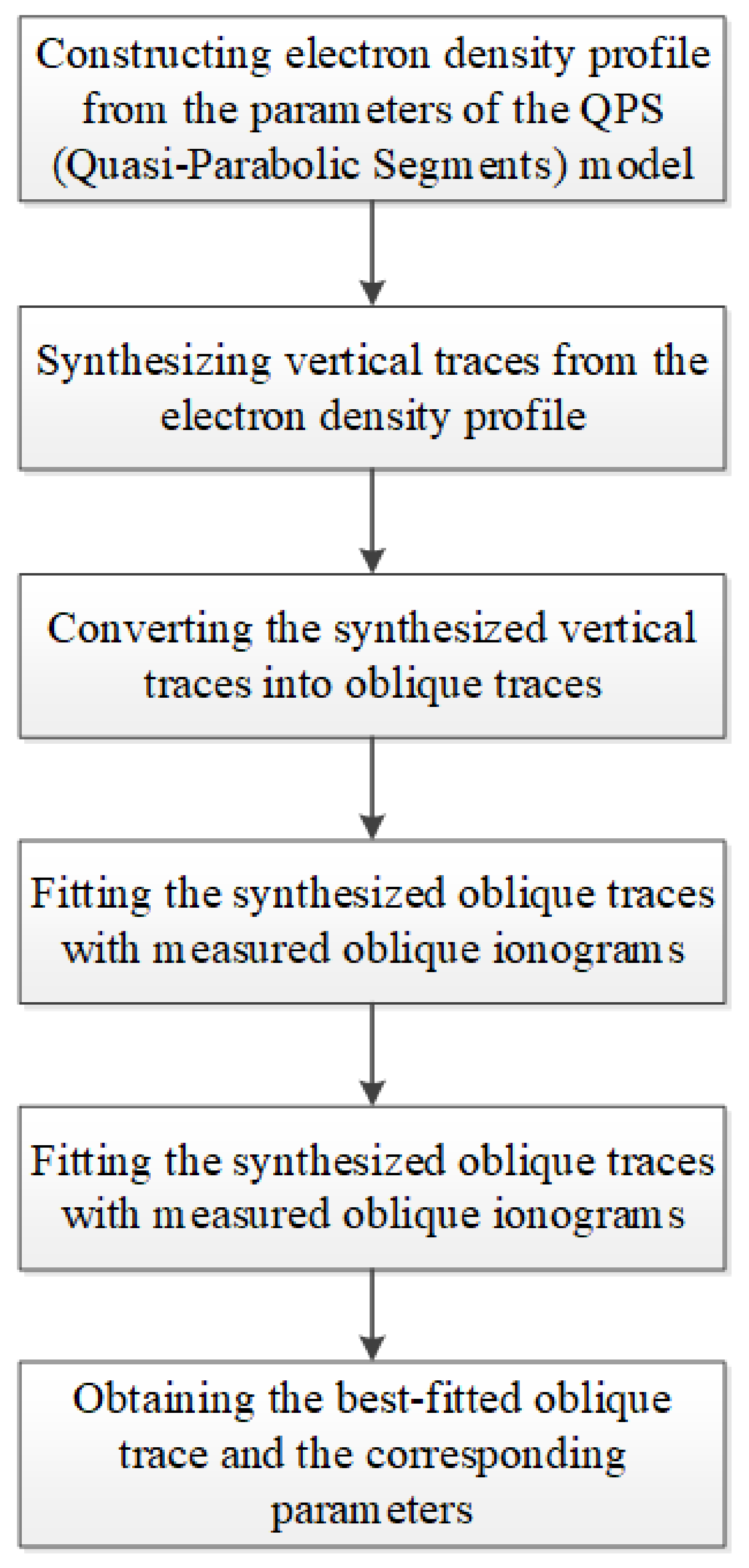
The quasi-parabolic segments model [21,22], widely used for inversion of vertical ionograms, was adopted to represent the ionosphere in this study. Then, vertical ionograms could be synthesized by the integral of group refraction index along the propagation path in the ionosphere. Furthermore, synthesized vertical ionograms could be transformed to oblique ionogram by the secant theorem and Martyn’s equivalent path theorem [23,24]. The synthesized oblique ionograms were further fitted to the measured oblique ionogram. Similar to automatic inversion of vertical ionograms by Jiang et al. [25,26], the initial nine parameters of QPS were determined from the IRI [27] and NeQuick model [28], and then adjusted to obtain a large amount of candidate oblique traces. Last, the best-fitted trace and parameters could be selected as the best-fitted output of automatic inversion of the oblique ionogram. Figure 1 shows the flowchart of the automatic inversion of oblique ionograms.
2.1. Automatic Scaling Key Parameters from Measured Oblique Ionograms
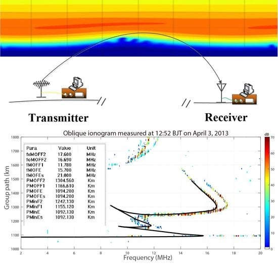
In the practical application, autoscaled parameters from measured oblique ionograms could be used to reduce the size of candidate traces. Therefore, the proposed method first automatically scaled the key parameters (the maximum observable frequency and minimum group path) from measured oblique ionograms. Similar to automatic scaling of vertical ionograms [10,25,26], the searching window and image projection techniques proposed by Jiang et al. [25,26] could also be utilized to scale oblique ionograms. The image projection technique is similar to the histogram technique by Lynn [29]. At first, the same technique as the ionoScaler software [10] was utilized to automatically extract the maximum observable frequency (MOF) and minimum group path of the E/Es (Sporadic E layer), F1, and F2 layer from oblique ionograms. Figure 2 shows a typical oblique ionogram recorded at 13:07 LT on 3 April 2013 between Beijing (40.3° N, 116.25° E) and Wuhan (30.5° N, 114.37° E). The black lines (on the horizontal and vertical axes) in Figure 2, respectively, represent the projection values at the Frequency and group path. As shown in Figure 2, the measured oblique ionogram could be divided into three regions (please see the back line on the vertical axis in Figure 2) according to the characteristics of the image projection at the group path. The maximum observable frequency could be identified by the projection values on frequency (please see the back line on the horizontal axis in Figure 2). Therefore, the searching window could be used to scale the maximum observable frequency and minimum group path for the E/Es, F1 and F2 layer. Therefore, we first defined the size of the searching window on measured oblique ionograms. Generally, the transmitter and receiver stations are known in the oblique sounding mode of the ionosphere. Then, the ground distance between the transmitter and receiver stations was adopted to determine the searching window in this study.
The searching window as , proposed by Jiang et al. [10,25,26], was represented by Equation (1):
where is the horizontal size of the searching window, is the resolution of the frequency in oblique ionograms, is the maximum height of the searching window, is the minimum height of the searching window, and is the resolution of the group path in oblique ionograms.
The present method defined as the width of the working frequency (2–15 MHz). The values of and varies depending on the E and F layers.
For the E/Es and F2 layer, the size of the searching window was represented by Equation (2).
where is the ground distance between the transmitter and receiver stations, is the peak altitude of the E layer from the IRI model, and and , respectively, are the deviation values of the group path of the E layer and F layer in oblique ionograms.
Once the searching window was defined, the image projection values of the searching window [26] were used to calculate the frequency and group path parameters of the E/Es and F layer from measured oblique ionograms. The detail procedure is similar to the methods proposed by Jiang et al. [26] and Song et al. [20]. In this study, we mainly introduce additional routines for identification of the Es and E layers in the present method.
For the Es layer, the proposed method first scaled the maximum observable frequency of the E/Es layer (fMOF_E_Es) from measured ionograms. Then, the fMOF_Emodel was calculated by the secant theorem and Martynˈs equivalent path theorem, where the parameters of E layer were estimated from the IRI model. The scaled parameter fMOF_E_Es was further compared with the fMOF_Emodel. If the fMOF_E_Es was larger than the fMOF_Emodel, we suggest that the Es layer existed in measured oblique ionograms. Otherwise, the proposed method suggested that no Es layer occurred in oblique ionograms. Since the altitude of the Es layer was close to the E layer, if the Es layer existed, the group path of the Es layer was suggested to be equal to the E layer in this study. Figure 3 shows the flowchart for estimating the parameters of the E and Es layer from measured oblique ionograms.
In measured oblique ionograms, the echoes of the F1 layer usually do not develop well compared with the E and F2 layers. Thus, the parameters of the F1 layer are estimated from the IRI and NeQuick models, but not from measured ionograms in this study. As a result, the frequency and group path parameters of E, Es, F1 and F2 layers could be estimated from measured oblique ionograms.
2.2. Synthesizing Oblique Ionogram through the QPS Model
The secant theorem and Martyn’s equivalent theorem could be used to study the relationship between the vertical ionogram and oblique ionograms. Many studies [20,30] used these theorems to convert oblique ionograms into vertical ionograms. On the contrary, vertical ionograms were required to be converted into oblique ionograms by the secant theorem and Martynˈs equivalent theorem in this study. Equation (3) was adopted to convert vertical traces into oblique traces.
where and , respectively, represent the frequency and group path in synthesized oblique traces, is the ground distance between the transmitter and receiver stations, is the virtual height of vertical traces, and is the frequency of vertical traces.
Figure 4 shows a typical synthesized vertical trace (left) and the converted oblique trace (right). The red line in the left panel of Figure 4 is the electron density profile represented by the QPS model with the parameters by Equation (4). The ground distance between transmitter and receiver stations was set to 1000 km.
2.3. Matching Measured Oblique Ionograms with Synthesized Oblique Traces
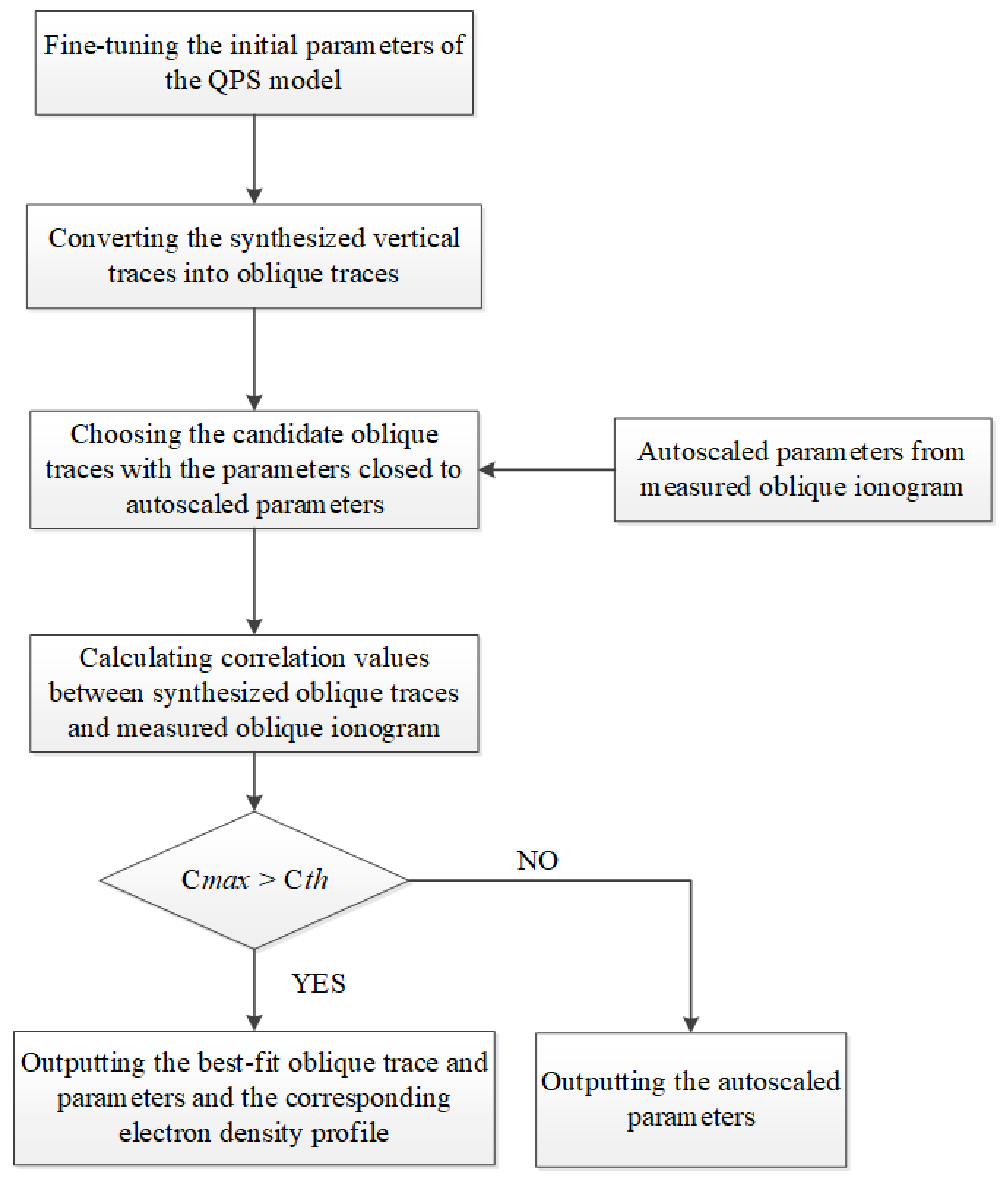
Similar to studies of vertical ionograms [26], a large amount of candidate vertical traces could be synthesized by the QPS model in this study. Reasonably, the range of the parameters of the QPS model in this study is similar to the reconstruction of vertical traces [26]. Furthermore, these candidate vertical traces could be transformed to oblique traces. Then, the synthesized oblique traces, whose parameters are close to autoscaled parameters, would be selected as the candidate traces to carry out correlation with measured oblique ionograms. It can reduce the running time of the proposed method to meet the near real-time application associated with inversion of oblique ionograms. Then, the correlation values between synthesized traces and the measured oblique ionogram were compared with the threshold value . If there were some correlation values larger than the threshold value , the oblique trace with the maximum correlation value and the corresponding parameters would be selected as the best-fitted one. Otherwise, the proposed method would output the autoscaled parameters mentioned above in Section 2.1. Figure 5 shows the flowchart of matching measured oblique ionograms with synthesized oblique traces.
3. Results
Figure 6 shows a best-fit synthesized trace (a black line) with the best-fit parameters on a measured oblique ionogram. This typical oblique ionogram includes the echoes of the Es layer. Result shows that the proposed method performed well for automatically scaling the parameters of the E, Es, F1 and F2 layers from oblique ionograms. Because the parameters of the F1 layer were estimated from the model, the synthesized trace did not match well for the echoes of the F1 layer. However, results suggested that it could not affect the performance of the matching trace of the E, Es and F2 layer. The proposed method is inspiring for automatic inversion of measured oblique ionograms, especially for the E/Es layer and F2 layer.
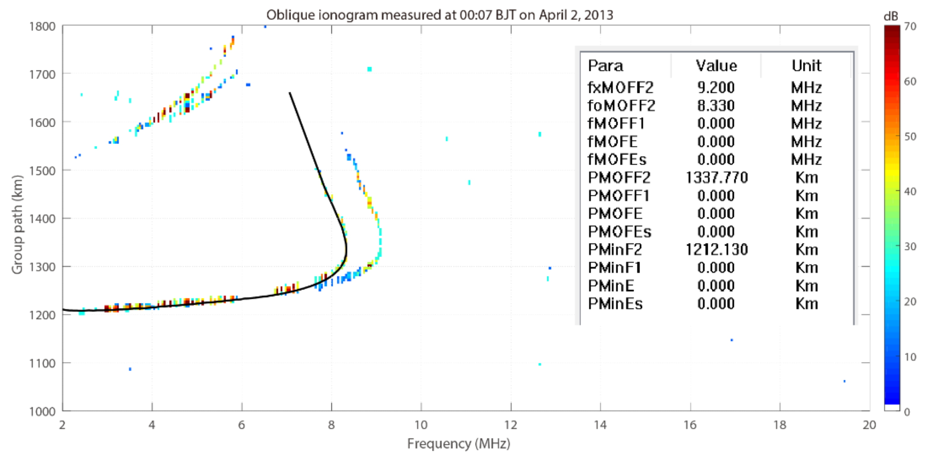
To test the feasibility of this method on different kinds of oblique ionograms, measured oblique ionograms were divided into three categories. The first category is ionograms with the Es layer and F1 layer, the second is without the F1 layer and Es layer, the third is with the F1 layer but without the Es layer. Figure 6 shows the first case. In this section, the second and third cases were tested. Figure 7 shows the best-fitted traces on measured oblique ionograms without the F1 layer and Es layer. Figure 8 shows the third case with the F1 layer but without the Es layer. It can be seen in Figure 7 and Figure 8 that the synthesized oblique traces (black lines) matched well on the echoes of oblique ionograms. The autoscaled parameters were also plotted in Figure 7 and Figure 8. Results matched well on different kinds of measured oblique ionograms, which inspired us to carry out a statistical study of autoscaled parameters on a large amount of oblique ionograms.
Because there are no ionosonde installed at the middle point between Wuhan and Beijing stations, the electron density profile inversed from measured oblique ionograms was not used to test the accuracy of the proposed method. It is well known that the parameters of the F2 layer are of great significance for the propagation of radio waves in the ionosphere. Therefore, the maximum observable frequency (maximum frequency of the observed trace) and the minimum group path of the F2 layer were utilized to verify the performance of this method. In this test, the parameters of fxMOFF2, foMOFF2, and PminF2 were adopted. In the presented method, the Es layer was identified by comparison with the E layer from the IRI model. It is difficult to directly identify the Es layer from measured oblique ionograms by operators when the most observed frequency is not large enough. Thus, the maximum observable frequency and the minimum group path of the E or Es layer were used to test the accuracy of autoscaled data. In the case of the E or Es layer, the operator would scale the maximum observable frequency and minimum group path of the echoes of the E or Es layer, but cannot identify that it is the E or Es layer. For autoscaled parameters, if the Es layer was identified, its parameters would be used to compare with manual scaled values. Otherwise, the autoscaled parameters of the E layer would be adopted. As a result, there are five parameters (fxMOFF2, foMOFF2, PminF2, fMOFE, PminE) from oblique ionograms. For measured oblique ionograms, the resolutions of working frequency and the group path are, respectively, 0.05 MHz and 5 km. Thus, an autoscaled value is considered to be acceptable if its error is within MHz for the frequency and km for the group path, which is in line with the URSI limits of ( is the reading accuracy).
Figure 9 and Figure 10 report the differences between the autoscaled values of the method described here and the standard manual values (Figure 9 for the parameters of the F2 layer, and Figure 10 for the E/Es layer). Table 1 illustrates the percentages of error statistical distributions of parameters for these differences. The accuracy of autoscaled frequency of the F2 layer is above 90%. However, the accuracy of the autoscaled group path is relatively lower (about 86.41%) compared with the maximum observable frequency. Due to the existence of the F1 layer, it is difficult to specify the minimum group path of the F2 layer. On the contrary, the accuracy of the autoscaled minimum group path of the E layer is higher (96.75%) than the autoscaled maximum observable frequency (60.05%). It is noted that the strength of the echoes of the E layer in these measured oblique ionograms are mostly lower, sometimes it is hard to accurately specify the maximum observable frequency of the E layer by the operator (see Figure 8). This will greatly affect the accuracy of autoscaled frequency of the E layer. Therefore, that is the reason that why the accuracy of the maximum observable frequency of the E layer is much less than the F2 layer. For the minimum group path, the lower strength of the echoes of the E layer would not affect the accuracy due to the projection values of the echoes of the E layer at the group path. Thus, we can see that the accuracy of the autoscaled group path for the E layer is high enough. On the contrary, the exact definition of the minimum group path plays a significant role on the accuracy of the autoscaled group path of the F2 layer. In this aspect, the E layer has a greater advantage compared with characteristics of the echoes of the F2 layer. That is the reason why the accuracy of the autoscaled group path of the E layer is greater than the F1 layer. For the lower accuracy of the maximum observable frequency of the E layer, the accuracy of the F2 layer inspires us to believe that it will be improved greatly if the echoes of the E layer are strong enough.
4. Conclusions
This study describes a method for automatic inversion of oblique ionograms. The proposed method first determined the initial autoscaled parameters using similar technologies of vertical ionograms proposed by Jiang et al. [25,26]. Then, a large number of candidate electron density profiles were constructed by the QPS model, based on the IRI model and the Nequick2 model. Furthermore, the candidate vertical traces, synthesized from electron density profiles, have been converted into oblique traces by the secant theorem and Martynˈs equivalent theorem. Lastly, these candidate oblique traces were used to obtain the best-fitted trace and parameters through matching measured oblique ionograms. Results show that the accuracy of the autoscaled frequency of the F2 layer is above 90% (91.98% for ordinary traces, 96.34% for extraordinary traces). The accuracy of the autoscaled group path is about 86.41%. For the E layer, the accuracy of the autoscaled minimum group path of the E layer can reach up to 96.75%. However, the accuracy of the autoscaled maximum observable frequency is relatively lower (about 60.05%) due to the lower strength of the echoes of the E layer. This indicates that the proposed method might be accurate enough for automatic inversion of oblique ionograms, especially for oblique ionograms with strong echoes (the F2 layer in this study). Results inspire us to develop and improve the performance. The proposed method still requires some adjustments to improve its accuracy and performance, and future studies will focus on the application of the proposed method at different geographic locations.
Author Contributions
Data curation, Z.C. and X.Z.; methodology, C.J.; software, C.J.; validation, C.J., G.Y. and T.L.; investigation, C.Z. and C.J.; writing—original draft preparation, C.J.; writing—review and editing, C.J. and Z.Z.; project administration, C.J. and Z.Z.; funding acquisition, T.L. and C.J. All authors have read and agreed to the published version of the manuscript.
Funding
This research was funded by the National Natural Science Foundation of China (NSFC), grant number 42074184, 41727804, 42104151, 41604133; Youth Foundation of Hubei Provincial Natural (No. 2021CFB134); and the Special Fund for Fundamental Scientific Research Expenses of Central Universities (No. 2042021kf0023).
Institutional Review Board Statement
Not applicable.
Informed Consent Statement
Not applicable.
Data Availability Statement
Oblique ionograms data are available from Chunhua Jiang upon request ([email protected]).
Acknowledgments
We are grateful to the Editor and anonymous reviewers for their assistance in evaluating this paper.
Conflicts of Interest
The authors declare no conflict of interest.
References
- Reinisch, B.W.; Galkin, I.A.; Khmyrov, G.M.; Kozlov, A.V.; Bibl, K.; Lisysyan, I.A.; Cheney, G.P.; Huang, X.; Kitrosser, D.F.; Paznukhov, V.V.; et al. New Digisonde for research and monitoring applications. Radio Sci. 2009, 44, RS0A24. [Google Scholar] [CrossRef]
- Rietveld, M.T.; Wright, J.W.; Zabotin, N.; Pitteway, M.L.V. The Tromsø dynasonde. Polar Sci. 2008, 2, 55–71. [Google Scholar] [CrossRef] [Green Version]
- MacDougall, J.W.; Grant, I.F.; Shen, X. The Canadian advanced digital ionosonde: Design and results. In Report UAG-14: Ionospheric Networks and Stations, World Data Center A for Solar-Terrestrial Physics; UAG-104, Ionosonde Network Advisory Group: Lowell, MA, USA, 1995; pp. 21–27. [Google Scholar]
- Zuccheretti, E.; Tutone, G.; Sciacca, U.; Bianchi, C.; Arokiasamy, B.J. The new AIS-INGV digital ionosonde. Ann. Geophys. Italy 2003, 46, 647–659. [Google Scholar] [CrossRef]
- Shi, S.; Yang, G.; Jiang, C.; Zhang, Y.; Zhao, Z. Wuhan Ionospheric Oblique Backscattering Sounding System and Its Applications—A Review. Sensors 2017, 17, 1430. [Google Scholar] [CrossRef] [Green Version]
- Reinisch, B.W.; Huang, X. Automatic calculation of electron density profiles from digital ionograms: 3. Processing of bottomside ionograms. Radio Sci. 1983, 18, 477–492. [Google Scholar] [CrossRef]
- Zabotin, N.A.; Wright, J.W.; Zhbankov, G.A. NeXtYZ: Three-dimensional electron density inversion for dynasonde ionograms. Radio Sci. 2006, 41, RS6S32. [Google Scholar] [CrossRef] [Green Version]
- Pillat, V.G.; Guimaraes, L.N.F.; Fagundes, P.R.; da Silva, J.D.S. A computational tool for ionosonde CADI’s ionogram analysis. Comput. Geosci. 2013, 52, 372–378. [Google Scholar] [CrossRef]
- Scotto, C.; Pezzopane, M. A software for automatic scaling of foF2 and MUF(3000)F2 from ionograms. In Proceedings of the URSI 2002, Maastricht, The Netherlands, 17–24 August 2002. [Google Scholar]
- Jiang, C.; Yang, G.; Zhou, Y.; Zhu, P.; Lan, T.; Zhao, Z.; Zhang, Y. Software for scaling and analysis of vertical incidence ionograms-ionoScaler. Adv. Space Res. 2017, 59, 968–979. [Google Scholar] [CrossRef]
- Smith, M.S. The calculation of ionospheric profiles from data given on oblique incidence ionograms. J. Atmos. Terr. Phys. 1970, 32, 1047–1056. [Google Scholar] [CrossRef]
- Chen, J.; Bennett, J.A.; Dyson, P.L. Synthesis of oblique ionograms from vertical ionograms using quasi-parabolic segment models of the ionosphere. J. Atmos. Terr. Phys. 1992, 54, 323–331. [Google Scholar] [CrossRef]
- Phanivong, B.; Chen, J.; Dyson, P.L.; Bennett, J.A. Inversion of oblique ionograms including the earth’s magnetic field. J. Atmos. Sol. Terr. Phys. 1995, 57, 1715–1721. [Google Scholar] [CrossRef]
- Huang, X.; Reinisch, B.W.; Kuklinski, W.S. Mid-point electron density profiles from oblique ionograms. Ann. Geophys. Italy 1996, 49, 757–761. [Google Scholar] [CrossRef]
- Redding, N.J. Image understanding of oblique ionograms: The autoscaling problem. In Proceedings of the IEEE Australian and New Zealand Conference on Intelligent Information Systems, Adelaide, SA, Australia, 18–20 November 1996; IEEE: Piscataway, NJ, USA, 1996; pp. 155–160. [Google Scholar]
- Fan, J.; Lu, Z.; Jiao, P. The intelligentized recognition of oblique propagation modes. Chin. J. Radio Sci. 2009, 24, 528. (In Chinese) [Google Scholar] [CrossRef]
- Settimi, A.; Pezzopane, M.; Pietrella, M.; Bianchi, C.; Scotto, C.; Zuccheretti, E.; Makris, J. Testing the IONORT-ISP system: A comparison between synthesized and measured oblique ionograms. Radio Sci. 2013, 48, 167–179. [Google Scholar] [CrossRef]
- Ippolito, A.; Scotto, C.; Francis, M.; Settimi, A.; Cesaronl, C. Automatic interpretation of oblique ionograms. Adv. Space Res. 2015, 55, 1624–1629. [Google Scholar] [CrossRef]
- Heitmann, A.J.; Gardiner-Garden, R.S. A robust feature extraction and parameterized fitting algorithm for bottom-side oblique and vertical incidence ionograms. Radio Sci. 2019, 54, 115–134. [Google Scholar] [CrossRef]
- Song, H.; Hu, Y.; Jiang, C.; Zhou, C.; Zhao, Z.; Zou, X. An automatic scaling method for obtaining the trace and parameters from oblique ionogram based on hybrid genetic algorithm. Radio Sci. 2016, 51, 1838–1854. [Google Scholar] [CrossRef]
- Croft, T.A.; Hoogasian, H. Exact ray calculations in a quasi-parabolic ionosphere with no magnetic field. Radio Sci. 1968, 3, 69–74. [Google Scholar] [CrossRef]
- Dyson, P.L.; Bennett, J.A. A model of the vertical distribution of the electron concentration in the ionosphere and its application to oblique propagation studies. J. Atmos. Terr. Phys. 1988, 50, 251–262. [Google Scholar] [CrossRef]
- Gethinga, P.J.D.; Maliphant, R.G. Unz’s application of Schlomilch’s integral equation to oblique incidence observations. J. Atmos. Terr. Phys. 1967, 29, 599–600. [Google Scholar] [CrossRef]
- Reilly, M.; Kolesar, J. A method for real height analysis of oblique ionograms. Radio Sci. 1989, 24, 575–583. [Google Scholar] [CrossRef]
- Jiang, C.; Yang, G.; Zhao, Z.; Zhang, Y.; Zhu, P.; Sun, H. An automatic scaling technique for obtaining F2 parameters and F1 critical frequency from vertical incidence ionograms. Radio Sci. 2013, 48, 739–751. [Google Scholar] [CrossRef]
- Jiang, C.; Yang, G.; Zhao, Z.; Zhang, Y.; Zhu, P.; Sun, H.; Zhou, C. A method for the automatic calculation of electron density profiles from vertical incidence ionograms. J. Atmos. Sol. Terr. Phys. 2014, 107, 20–29. [Google Scholar] [CrossRef]
- Bilitza, D.; Altadill, D.; Truhlik, V.; Shubin, V.; Galkin, I.; Reinisch, B.; Huang, X. International Reference Ionosphere 2016: From ionospheric climate to real-time weather predictions. Soc. Work. 2017, 15, 418–429. [Google Scholar] [CrossRef]
- Nava, B.; Coisson, P.; Radicella, S.M. A new version of the NeQuick ionosphere electron density model. J. Atmos. Sol. Terr. Phys. 2008, 70, 1856–1862. [Google Scholar] [CrossRef]
- Lynn, K.J.W. Histogram-based ionogram displays and their application to autoscaling. Adv. Space Res. 2018, 61, 1220–1229. [Google Scholar] [CrossRef]
- Ippolito, A.; Scotto, C.; Sabbagh, D.; Sgrigna, V.; Maher, P. A procedure for the reliability improvement of the oblique ionograms automatic scaling algorithm. Radio Sci. 2016, 51, 454–460. [Google Scholar] [CrossRef]
Figure 1.
Flowchart of the automatic inversion of oblique ionograms.

Figure 2.
A typical oblique ionogram with projections at the group path and frequency recorded at 13:07 LT on 3 April 2013, between Beijing and Wuhan. The back lines on the vertical and horizontal axes, respectively, represent the projection values at the group path and frequency.
Figure 2.
A typical oblique ionogram with projections at the group path and frequency recorded at 13:07 LT on 3 April 2013, between Beijing and Wuhan. The back lines on the vertical and horizontal axes, respectively, represent the projection values at the group path and frequency.

Figure 3.
Flowchart of estimating the parameters of E and Es layer from measured oblique ionograms.

Figure 4.
A typical synthesized vertical trace (left) and the converted oblique trace (right); the red line in the left pane represents the corresponding electron density profile.
Figure 4.
A typical synthesized vertical trace (left) and the converted oblique trace (right); the red line in the left pane represents the corresponding electron density profile.

Figure 5.
Flowchart of matching measured oblique ionograms with synthesized oblique traces.

Figure 6.
Oblique ionogram measured at 12:52 BJT on 3 April 2013 with the best-fit synthesized trace (a black line) and best-fit parameters.
Figure 6.
Oblique ionogram measured at 12:52 BJT on 3 April 2013 with the best-fit synthesized trace (a black line) and best-fit parameters.

Figure 7.
Similar to Figure 6, but the oblique ionogram was measured at 00:07 BJT on 2 April 2013 without the F1 layer.
Figure 7.
Similar to Figure 6, but the oblique ionogram was measured at 00:07 BJT on 2 April 2013 without the F1 layer.

Figure 8.
Similar to Figure 6, but oblique ionogram was measured at 13:22 BJT on 2 April 2013 without the Es layer. Oblique ionograms measured during 8–16 April 2013 by the ionosondes between Wuhan and Beijing stations were used to carry out statistical analysis of the performance of the proposed method. The ground distance between Wuhan and Beijing stations is approximately 1040 km. The number of measured oblique ionograms is about 795.

Figure 9.
Error distributions of fxMOFF2, foMOFF2, and PminF2 for oblique ionograms between the manual and autoscaled values.
Figure 9.
Error distributions of fxMOFF2, foMOFF2, and PminF2 for oblique ionograms between the manual and autoscaled values.

Figure 10.
Similar to Figure 9, but for fMOFE and PminE.
Figure 10.
Similar to Figure 9, but for fMOFE and PminE.


Table 1.
The percentages of error statistical distributions of autoscaled parameters from oblique ionograms.
Table 1.
The percentages of error statistical distributions of autoscaled parameters from oblique ionograms.
| Item | fxMOFF2 | foMOFF2 | PminF2 | fMOFE | PminE |
|---|---|---|---|---|---|
| Acceptable values | 96.34% | 91.98% | 86.41% | 60.05% | 96.75% |
| Total number of oblique ionograms | 795 | ||||
Publisher’s Note: MDPI stays neutral with regard to jurisdictional claims in published maps and institutional affiliations. |
© 2022 by the authors. Licensee MDPI, Basel, Switzerland. This article is an open access article distributed under the terms and conditions of the Creative Commons Attribution (CC BY) license (https://creativecommons.org/licenses/by/4.0/).
Share and Cite
MDPI and ACS Style
Jiang, C.; Zhao, C.; Zhang, X.; Liu, T.; Chen, Z.; Yang, G.; Zhao, Z. A Method for Automatic Inversion of Oblique Ionograms. Remote Sens. 2022, 14, 1671. https://0-doi-org.brum.beds.ac.uk/10.3390/rs14071671
AMA Style
Jiang C, Zhao C, Zhang X, Liu T, Chen Z, Yang G, Zhao Z. A Method for Automatic Inversion of Oblique Ionograms. Remote Sensing. 2022; 14(7):1671. https://0-doi-org.brum.beds.ac.uk/10.3390/rs14071671
Chicago/Turabian StyleJiang, Chunhua, Cong Zhao, Xuhui Zhang, Tongxin Liu, Ziwei Chen, Guobin Yang, and Zhengyu Zhao. 2022. "A Method for Automatic Inversion of Oblique Ionograms" Remote Sensing 14, no. 7: 1671. https://0-doi-org.brum.beds.ac.uk/10.3390/rs14071671
Note that from the first issue of 2016, this journal uses article numbers instead of page numbers. See further details here.