Technical Note

Improved Ionosonde Monitoring of the Sporadic E Layer Using the Frequency Domain Interferometry Technique

1
School of Electronic Information, Wuhan University, Wuhan 430072, China
2
Institute of Space Science and Applied Technology, Harbin Institute of Technology, Shenzhen 518000, China
*
Author to whom correspondence should be addressed.
Submission received: 30 March 2022 / Revised: 13 April 2022 / Accepted: 13 April 2022 / Published: 15 April 2022
(This article belongs to the Special Issue Ionosphere Monitoring with Remote Sensing)

Abstract

:
The sporadic E (Es) layer is a thin layer of ion plasma enhancement in the E-region ionosphere, typically at altitudes of 90–120 km with vertical and horizontal extent of several or several tens of kilometers. As the transition region between the lower and upper atmosphere, this layer is of critical importance for ionospheric studies. The most economical but effective method to observe this layer is using ionosonde, which, however, is incapable of capturing the finer structure or the internal inhomogeneity of the Es layer as the range resolution is on the order of kilometers. To overcome this limitation, we employ the frequency domain interferometry (FDI) technique, a technique that has been successfully applied to the analysis of some radar and sonar measurements. Here, we use the Es layer measurements near Wuhan, China (114°22′E, 30°30′N) on 8 June 2021 as examples to showcase the capability of this technique. Our results show that the spatial resolution of ionosonde imaging is remarkably increased: the complexity of the internal fine structure in the Es layer can be well observed in the FDI-processed ionograms, whereas the intrinsic range resolution is several kilometers. Moreover, by comparing the ionograms obtained with and without the FDI technique, it is found that the FDI-processed ionogram is particularly suitable for the observation of evolutional processes in the Es layer, as well as the identification of different types of Es layer. With this level of spatial resolution, ionosonde, in combination with the FDI technique, opens the possibility for more refined observations of the Es layer.

Graphical Abstract

1. Introduction

The sporadic E (Es) layer is a relatively thinner (compared to other layers of the ionosphere) layer of enhanced ion plasma in the E-region ionosphere, typically at altitudes of 90–120 km with a vertical extent of several kilometers and a horizontal extension of several tens of kilometers [1].
The formation of the Es layer can be well explained by the wind shear theory and the convergence of metal ions [2,3,4]. Other than these, shear instabilities, tidal, planetary, or gravity waves, meteors, and thunderstorms could somewhat influence the electron density distribution in the Es layer as well [5,6,7]. For example, the Kelvin–Helmholtz instability (KHI) can lead to a billow structure and a polarization electric field in the Es layer [8,9]. Tidal and planetary waves can give rise to periodic vertical fluctuations in the Es layer [10,11]. Gravity waves can modulate the Es layer and cause distortions along both horizontal and vertical directions, which are ultimately recorded as quasiperiodic backscatter echoes in the very-high-frequency (VHF) range [12,13]. The seasonality of the Es layer is well related with the occurrence of meteors [14], and, as has been reported numerously, the Es formation in the mid-latitudes is also closely related to the sporadic metal layer [15]. The correlation between the spread F-region ionosphere, thunderstorms, and Es layer has implications for the coupling between the upper and lower layers of the Earth’s atmosphere as well [16]. Considering these, as the transition region between the lower and upper atmosphere, the morphological structure, composition, and temporal evolution of the Es layer has been the main focus of various theoretical and observational studies, and improving the spatial resolution of Es layer measurements is critical for better understanding the formation and evolution mechanism of the Es layer, as well as the above-mentioned atmospheric processes.
Up to now, although extensive observational efforts have been made, the vertical structure of the Es layer still remains insufficiently investigated due to its transient nature and limitations in observation techniques. By analyzing the in situ data measured during the campaign of Sporadic E Experiment over Kyush (SEEK), Mori and Oyama found that the Es layer can exhibit a complicated multiple layer structure at altitudes with the separation of 10–12 km [17,18,19]. This multilayer structure was later confirmed by Damtie et al. using the radio sounding data collected by the European Incoherent Scatter (EISCAT) radar [20]. The authors have specifically found that the electrons in the Es layer were distributed at multiple fine layers with spatial intervals of 1–2 km, and during the downward drifting phase, these fine layers were merged into a single layer. Using the EISCAT data, Turunen et al. have further investigated the undulating movement of the Es layer along the vertical direction and revealed that this layer could be compressed by plasma streams and degenerated owing to the fluctuations in the neutral atmosphere [21].
Along the horizontal direction, the Es layer is also found to exhibit many variations, and a “blanketing” or “patchy” structure is found in most cases [22]. The Es layer can be reconstructed via ionosonde using the critical reflection frequency and the direction of arriving waves, which can be utilized to image the embedded structure of field-aligned irregularities (FAIs) in the Es layer [23,24]. The incoherent scatter radar (ISR) images recorded by Hysell et al. have shown that the Es layer at middle latitudes could exhibit both cloud-like and wave-like structures [25]. As for the Es layer at higher latitudes, for example, in Alaska, Hysell et al. have revealed a two-dimensional “patchy” and “stripe” structure [26]. In addition to radar imaging, the Es layer has been extensively studied using measurements from space, for example, the Global Positioning System (GPS) [27], using the total electron content (TEC) anomalies [28].
Compared to other types of Es layer measurements, for example, ISR and GPS, ionosonde has the advantage of providing persistent observation at a relatively low cost. In particular, compared with ISR, large antenna array and great transmission power are not required, and unlike GPS, the bottom-up sounding of the ionosonde is not affected by the F layer, and even weak Es layers can be observed. However, the inhomogeneity of the fine structure of this layer cannot be well captured due to the poor range resolution of the ionosonde, and its applicability in studies of Es layer formation and evolution is limited. To overcome this limitation represents the main goal of this study and, for this purpose, we utilize the frequency domain interferometry (FDI) technique. We show that this technique, which was originally developed for the analysis of radar and sonar measurements [29], is also applicable to ionosonde measurements. In the following, we explain how this technique is utilized to process ionosonde data, and we use several examples of Es layer measurement to showcase the resolution improvement obtained using this technique.

2. Experiment Setup and Methods

2.1. Instruments and Experimental Setup

The ionosonde used in this study is a miniature version of the Wuhan Ionospheric Sounding System (WISS), as developed by the Ionospheric Laboratory of Wuhan University [30]. It specifically uses a 16-bit complementary coded sequence to modulate the high-frequency (HF) signals with a peak power of 500 watts and performs vertical incidence sounding. The transmission duration for any coded chip is 25.6 microseconds (μs), corresponding to an intrinsic range resolution of 3.84 km. In regular mode, each frequency-sweep sounding was performed for a total duration of ~3 min at frequencies from 2 to 20 megahertz (MHz) with steps of 0.05 MHz. The number of accumulations was set to be 32. After a 12 min interruption, the typical sounding period of the frequency-sweep detection was 15 min, which is sufficient for general ionospheric observation missions. The WISS uses an inverted-V-shaped antenna for signal transmission and another 30 m three-wire antenna for signal reception. Therefore, during conventional detection, ordinary (O) and extraordinary (X) modes of ionogram echo traces can be distinguished using image processing [31]. It is worth mentioning that WISS has been widely deployed in China and provides reliable data for various ionosphere studies [32].
To ensure good coherence, i.e., reflection of adjacent frequencies at the same height, the frequency step of the ionosonde was set to be 10 kilohertz (kHz) during this experiment. The number of accumulations at each frequency point was 256 since this number provides sufficient samples for the next-step FDI processing. The resident time of each frequency point is about 4.19 s. We emphasize that the time consumption caused by smaller frequency intervals would not significantly affect the Es detection since the Es layer at low and middle latitudes, in general, can last for at least tens of minutes [14,26]. The sounding frequency range in this experiment was set to be 2–4 MHz, as typically needed for good resolution of the Es layer, also taking into account the acceptability of the time consumption. Thus, the ionosonde sounding period was still approximately 15 min, which is consistent with the conventional ionospheric vertical sounding period. Similarly, also in accordance with the conventional ionospheric vertical measurements, short-term changes in the internal structure of the Es layer during the detection period (15 min) are temporarily ignored. Therefore, this paper is more inclined to reflect the relatively static inhomogeneity of the fine structure of Es layer and the evolution process of a 15 min level. The experiments reported in this study were performed near Wuhan, China (114°22′E, 30°30′N, geomagnetic dip angle: 45°) on 8–9 June 2021. During this period, the Kp indexes are less than 2 [33], which means a geomagnetically quiet day.

2.2. Es Layer Imaging Based on the FDI Technique

The FDI technique has been successfully applied to the analysis of atmospheric radar measurements of ionospheric turbulence and FAIs [34,35]. Good performance has been obtained in general, although with the following drawback: while using a limited number of frequency points to image a small vertical extent, the observation results can only reflect the target response characteristics at a certain frequency band. To remedy this drawback, different from previous radar studies, we first process the frequency-sweep-detected echoes of the Es layer in a wide frequency range. The FDI technique of ionosonde data processing is then applied in the following procedure.
The Es layer is assumed as a target with a slow movement and a narrow height distribution; therefore, when a series of adjacent frequencies is used for sounding and the changes in the Es characteristics in a short duration are ignored, the echo signal S p ( t ) of frequency f p is expressed as
S p ( t , r ) = A p s ( t 2 r / c ) · e j 2 π f p ( 2 r / c ) + φ p
where c represents the speed of light, A p represents the echo amplitude, s ( · ) expresses the echo envelope, r is the radial distance, and φ p is the initial phase. For a coherent radar system such as the WISS, the initial phase of the transmission signal in a small frequency band can be assumed to be the same; thus, for similar working frequencies, the echo phase difference of the same target must meet the following condition:
Δ ϕ = 2 π · 2 r c · ( Δ f )
where Δ f represents the frequency interval. The phase difference is only related to the distance of the target and the frequency interval. The unambiguity range of the signal phase is 2 π , and subsequent processing is performed based on the order of the range gate; thus, it is necessary to ensure that no phase ambiguity occurs within a range resolution unit. The frequency step Δ f 0 during sounding should satisfy the following condition:
Δ ϕ = 2 π · 2 r 0 c · ( Δ f 0 ) 2 π Δ f 0 c 2 r 0
where r 0 represents the initial range resolution of the ionosonde radial distance. This resolution is 3.84 km for the WISS, indicating that Δ f 0 must be smaller than 39.0625 kHz. The frequency step of 10 kHz selected in our experiment clearly meets the requirement.
The signal matrix for the echo signals of a certain frequency f p and the following k adjacent frequencies f p ~ f p + k , ( f p 4   MHz k · Δ f ) is constructed as follows:
S ( t , r ) = [ S p ( t , r ) , S p + 1 ( t , r ) , , S p + k ( t , r ) ] T
where [ · ] T represents the matrix transpose. For each range gate, the echo data of each frequency are extracted, and the covariance matrix R S is calculated as Equation (5):
R S = S S H / n
where n = 256 is the accumulation number in our experiment, and [ · ] H represents the conjugate transpose of the matrix. A range-dimensional steering vector is determined based on the required resolution:
{ a ( f p , r 1 ) = [ e j 2 π f p ( 2 r 1 / c ) , e j 2 π f p + 1 ( 2 r 1 / c ) , , e j 2 π f p + k ( 2 r 1 / c ) ] H a ( f p , r 2 ) = [ e j 2 π f p ( 2 r 2 / c ) , e j 2 π f p + 1 ( 2 r 2 / c ) , , e j 2 π f p + k ( 2 r 2 / c ) ] H a ( f p , r m ) = [ e j 2 π f p ( 2 r m / c ) , e j 2 π f p + 1 ( 2 r m / c ) , , e j 2 π f p + k ( 2 r m / c ) ] H
where r s is defined as the expected resolution, and m = r 0 / r s represents the refined factor.
Therefore, based on the data of each range gate with the initial resolution, the spectrum of the j th refined range unit can be estimated using the Capon method:
b ( f p , r j ) = 1 a H ( f p , r j ) R s 1 a ( f p , r j ) , j = 1 , 2 , , m
The sounding range resolution can be increased by m times by scanning the range spectrum. Essentially, it is a type of spectrum estimation method in the range dimension that uses the coherence between the echo signals of the same target in the frequency domain.
In this study, we performed the frequency-sweep sounding of the Es layer using the FDI technique in a frequency steeping mode. Considering the observational frequency range of 2–4 MHz, the electromagnetic environments of each frequency were differed slightly, possibly inducing severe interference during the spectral estimation. For enhanced frequency scanning imaging, we normalized the spectral estimation results and used a Gaussian window to perform range smoothing. Eleven adjacent frequencies were considered in one run of the spectral estimation ( k = 11 ). The scanning step of the range spectrum was set to 38.4 m ( m = 100 ). Note that because the maximum frequency interval of the signals used in one imaging process was only 100 kHz, the difference in the phase-frequency response of the system between the adjacent frequencies was not considered to induce severe adverse effects to the range spectral estimation.
Inevitably, for a single-channel ionosonde, using a wide beam antenna, it is difficult to have the capabilities of direction-estimating and beam-pointing. Naturally, it is impossible to accurately locate the target position. In spite of this, it should be feasible to use this method to monitor the inhomogeneity and complexity of the internal structure of the Es layer. If the Es layer is dense and uniform, the imaging result should also be a narrow thin line. This is because when the signal is not vertically incident, it will be reflected to other directions and will not return to the ionosonde. On the contrary, if the Es layer is inhomogeneous, due to the unsmooth lower boundary of the Es layer or the presence of embedded irregularities, the diffuse range spectrum should be obtained.

3. Results

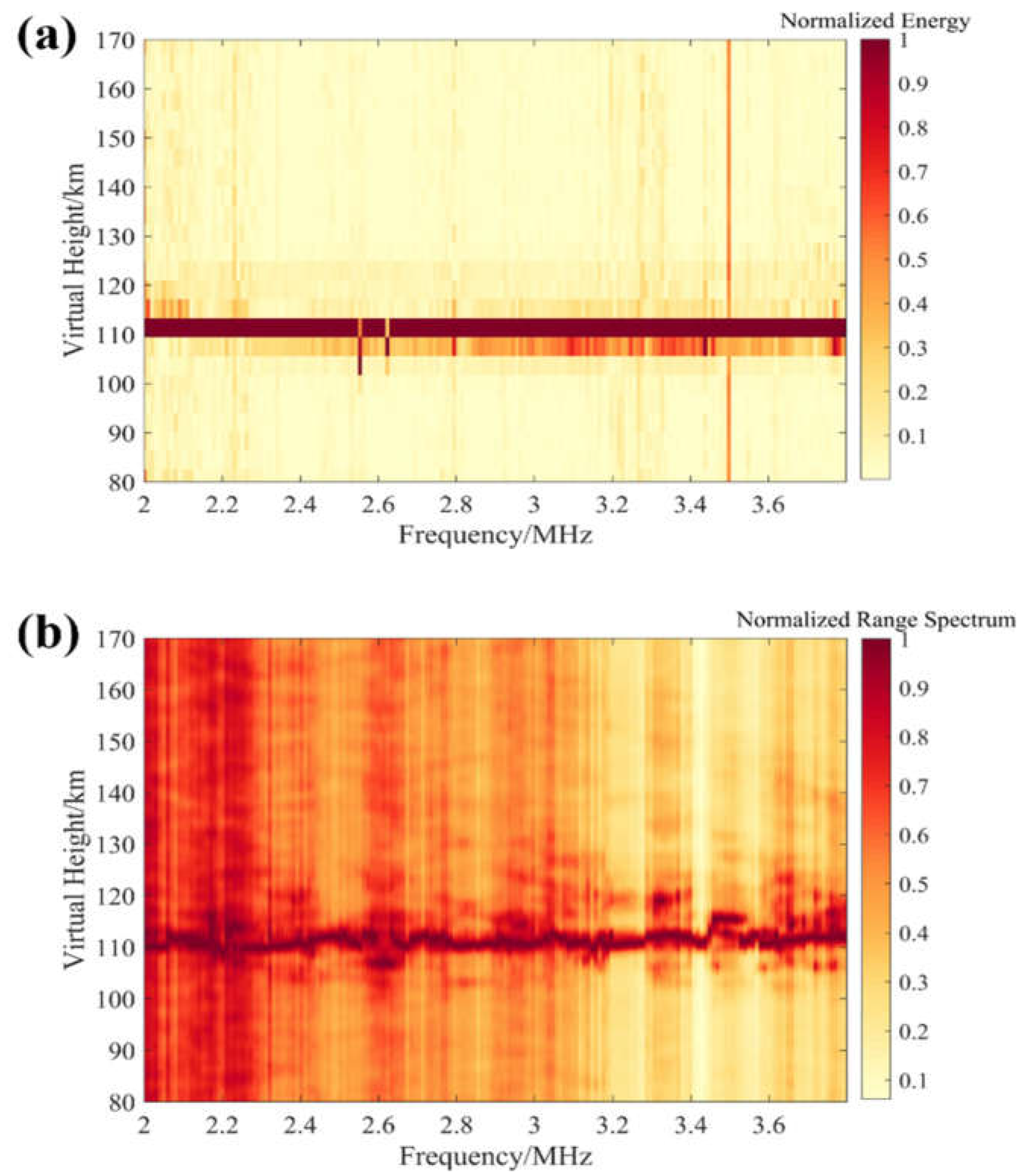
3.1. The Inhomogeneous Es Layer

Figure 1a shows the height–intensity ionogram of the Es layer measured near Wuhan, China (114°22′E, 30°30′N) at 17:46 LT (UTC+8) on 8 June 2021. Figure 1b shows the normalized energy at different altitudes and frequencies, while Figure 1c shows the FDI-processed ionogram with a range resolution of 38.4 m. The FDI technique needs more than one frequency point to ensure good coherence, and thus the frequency points close to the upper boundary of present ionogram cannot be well imaged. As such, in this paper, only the part of frequencies below 3.8 MHz were FDI-processed, which is shown in Figure 1b,c for comparison.
According to International Reference Ionosphere (IRI) 2016 [36], at this time, the peak height of E layer is 110 km and the critical frequency is 1.7 MHz; therefore, Figure 1 shows a diffuse Es layer, for which imaging results do not focus on a certain range. The reflection height corresponding to the strongest energy was approximately 107 km with the smaller echoes distributed at altitudes of 103–123 km. It is clear from Figure 1a,b that, with the intrinsic resolution of 3.84 km, it is almost impossible to recognize the fine structure and diffusion features. In contrast, the echoes due to smaller-scale electron density irregularities (as circled by the dotted blue line) are clearly shown in Figure 1c. The virtual height of the sounding echoes dramatically changes at varying frequencies, as shown in Figure 1c. A direct comparison between Figure 1a–c shows the improvement of spatial resolution of the FDI technique. At the same time, it can also be observed from Figure 1c that this is a highly inhomogeneous Es layer.

3.2. Quiet Es Layer

In addition to the diffuse Es layer shown in Figure 1, we have also examined the FDI method during quiet Es conditions, as shown in Figure 2. Figure 2a shows an example of quiet Es condition measured by WISS near Wuhan, China at 22:34 LT (UTC+8) on 8 June 2021. The echo trace of the Es layer is a clear and uniform straight line, indicating that the Es layer is dense and stable at this time. In this sense, it can be regarded as quiet. Figure 2a,b show the ionograms obtained without and with applying the FDI technique. The corresponding range resolution is 3.84 km and 38.4 m, respectively. From the comparison between these two panels, it is clear that the sounding echoes are almost flat at ~110 km altitude as in the conventional ionogram (Figure 2a), while smaller-scale fluctuations are resolved in the FDI-processed ionogram (Figure 2b).

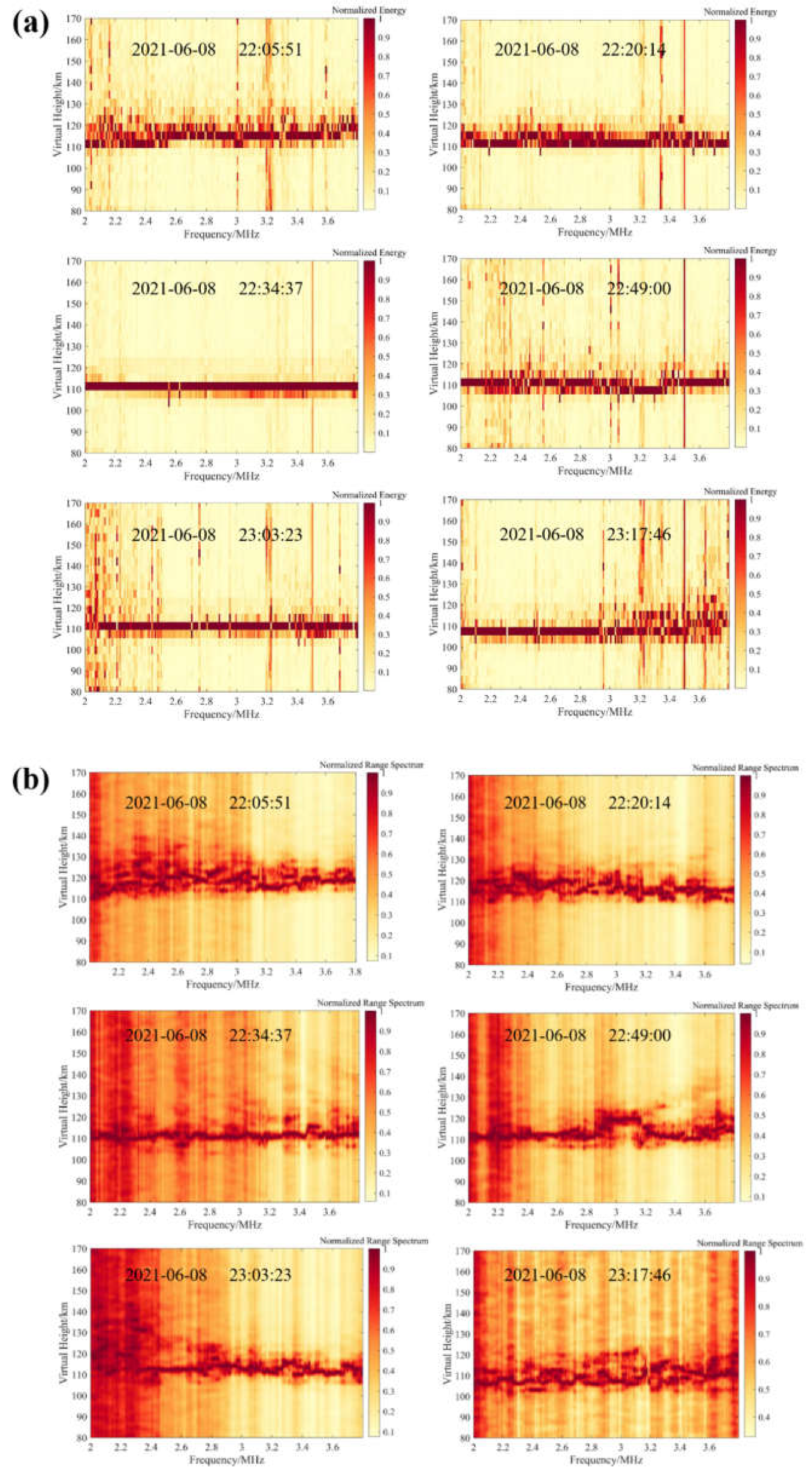
3.3. Short-Term Evolution of the Es Layer

Figure 3a shows the ionograms measured between 22:06 and 23:18 LT (UTC+8) on 8 June 2021. Figure 3b shows similar results, but obtained using the FDI technique with a range resolution of 38.4 m. During this time interval, the echo trace was first compressed and then expanded, implying that the Es layers are evolving from a thin layer to inhomogeneously distributed irregularities. This example somewhat resembles the event recorded by Hysell et al. using ISR [29]. The evolutional process is hardly recognizable in the conventional ionograms, whereas how it was compressed and expanded is clearly resolved in Figure 3b.

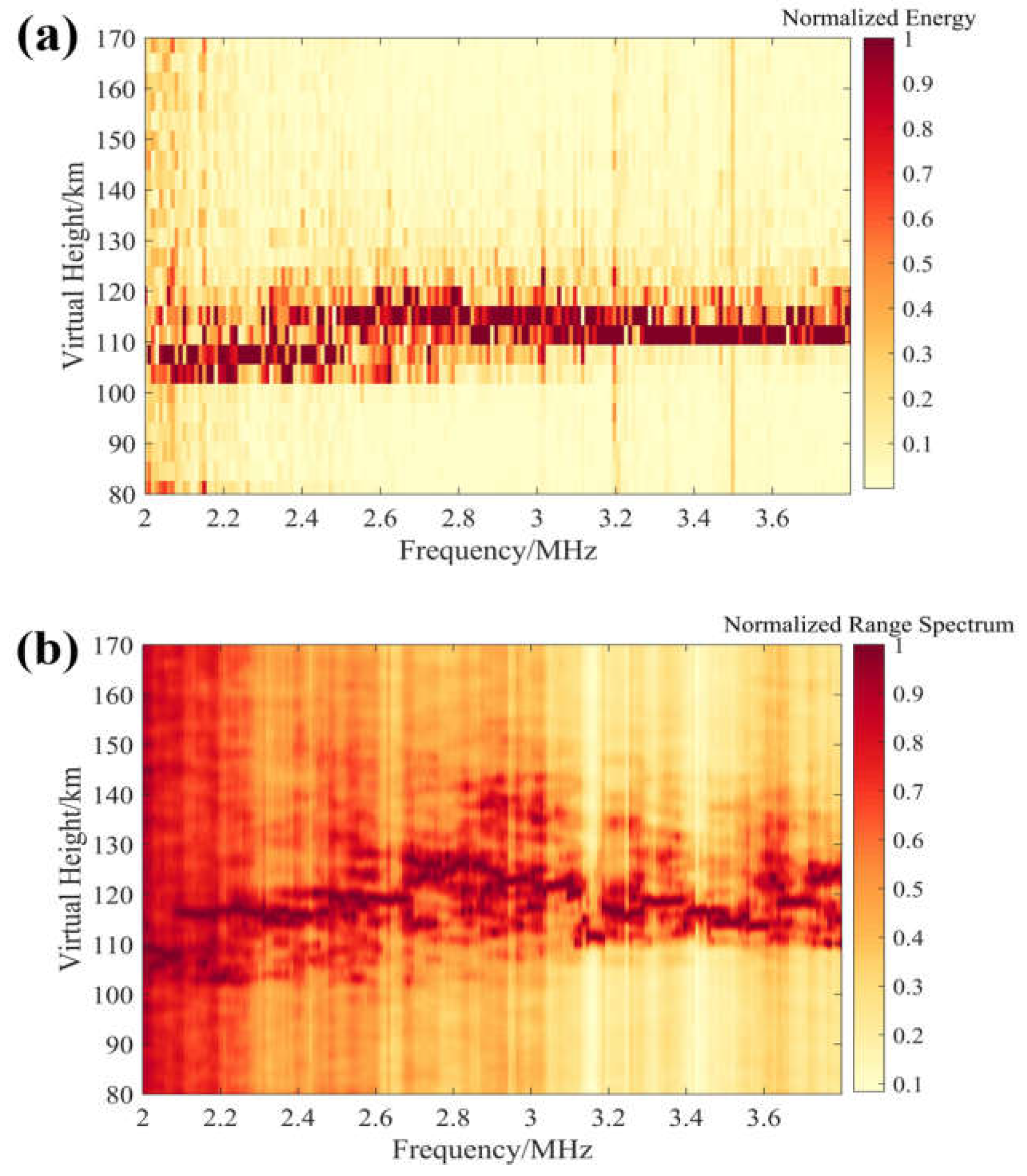
3.4. Different Types of Es Layer

The proposed FDI technique is also particularly suitable for the identification of different types of Es layer, especially in a relatively narrow frequency band.
Figure 4a shows the conventional ionogram measured at 19:56 LT on 8 June 2021. Figure 4b shows the same event but obtained using the FDI technique. The echo trace at frequencies of 2.4–2.7 MHz shown in Figure 4a is indicative of a multilayer structure, but it is difficult to determine which type of Es layer was recorded. On the other hand, after applying the FDI technique, it is found that the traces of the Es layers were connected and the traces at 2.4–2.6 MHz exhibited a continuous “spike” shape; both features suggest a c(cusp)-type Es layer according to the manual of ionogram scaling [37].
Another example is shown in the bottom two panels of Figure 4. These two panels show the Es layer measured at 01:12 LT on 9 June 2021. Based on the conventional ionogram (Figure 4c), the Es layer was likely l (low)-type. Nevertheless, after being processed using the FDI method, this Es layer is actually found to be the h (high)-type (Figure 4d) with no “symmetrical spikes”. The upper and lower traces are likely to represent the Xmode and O-mode.

4. Discussion

In Figure 1c, at frequencies lower than 3.2 MHz, diffused range spectra of the echoes were patchily distributed at altitudes of 100–115 km. This reflects the complexity of the internal structure of the Es layer at this time, and the electron density distribution is obviously inhomogeneous. As the spectral peaks are obvious and separated from each other, there may be discontinuous and drastic changes in the spatial distribution of the internal electron density. A reasonable explanation for this phenomenon is, as Whitehead suggested [23], electron density irregularities that are embedded in the Es layer and can considerably scatter the sounding signals. The spectral intensity of the scattered echoes can even suppress the reflected signals at certain frequencies. The inconsistency in terms of the scatterers’ position and scale could thus extend the intensity spectra in both range and frequencies. The echo trace between 3.2 and 3.8 MHz is typical of the ionosonde reflection mode and the signal echo height was divided into two layers, indicating an internal multilayer structure with intervals of ~5 km which are likely semi-shielded by each other. Note that the higher layer should not be suspected as caused by the interference due to the reflected waves from nearby objects within the irradiation range of the antenna beam. If this were the case, continuous multilayer echoes would show up in the low-frequency band as well. This feature is more in line with the partial reflection theory and hole structures of the Es layer along the horizontal direction [38,39]. However, this hypothesis needs to be further examined by using a two-dimensional imaging technique or measuring the incoming direction of the signals for positioning with an antenna array.
As for Figure 2b, these fluctuations are reflective of a weak inhomogeneity distribution of electrons in the Es layer. Of special interest is the virtual heights at 2.6 and 3.5 MHz, which are either higher or lower than the overall trend, and not captured by the conventional ionogram (Figure 2a). In other studies, using the ISR data, such phenomena had also been confirmed to exist in the Es layer [29]. This example also demonstrates that the spatial resolution of the ionosonde is largely increased and the FDI technique can be well used to study the physical processes involved in the formation and evolution of the Es layer. Note that this level of spatial resolution can also be achieved using ISR, but with the cost of much higher power consumption and larger antenna array.
Based on Figure 3b, it is worth noting that the compression speed of the echo trace is faster than that of rediffusion. It can be observed that the diffusion range of the spectral virtual height was compressed from 20 km to a thread with slight jitters, continuous echo traces in <15 min, probably indicting that the Es layer evolved from an uneven structure to a dense and uniform layer. For the echoes of different frequencies, the compression process on the imaging ionogram proceeded at basically the same speed. However, rediffusion started from the high-frequency band. At 3.2–3.8 MHz, the traces first showed folds and then extended to the low-frequency band. A reasonable explanation for this could be that the uniform and dense Es layer first yielded small fragments due to the instability or modulation of atmospheric gravity waves and then broke into patches and drifted. This observation indicates an Es variation from “blanketing” to “patchy”, and vice versa, which can be temporally dynamic and unstable. These findings obtained within ~1 h indicated a relatively drastic short-term disturbance in the Es layer. Although it remains unclear whether KHI caused by the strong shear of the background neutral wind led to the formation of the unstable patchy Es and FAIs [8] or the wind field of the gravity waves [29] or the internal instability caused by the polarization electric field [9,40,41,42] is the dominant mechanism, the FDI technique based on ionosondes can provide a new, convenient, and promising way of investigating this open question.
The effect of Figure 4 reveals that there may be some uncertainties in the ionosonde measurements, as caused by the coarse resolution of conventional ionograms. The FDI technique is thus more suitable for Es layer identification. Note also that the virtual heights of the echo traces in Figure 4b at 2.2–2.4 MHz and in Figure 4d at 2.4–2.6 MHz are higher than their corresponding positions in Figure 4a,c, respectively. This is because although the energy of the echoes at the lower position is strong, they mainly originate from different scatters, and the coherence between the signals at different frequencies is not prominent. Alternatively, the higher echoes in Figure 4b,d are due to the reflected signals, suggesting that good coherence leads to an enhanced-range spectral estimation.

5. Conclusions

In this study, we employ the FDI technique to improve the spatial resolution of ionosonde measurements. Using the Es layer measurements near Wuhan as examples, our results show that the spatial resolution of height–intensity ionograms is remarkably increased: the complexity and inhomogeneity of the internal fine structures can be well monitored in the FDI-processed ionograms, compared to the intrinsic range resolution of several kilometers. Moreover, it is found that the detailed evolutional processes and different types of Es layer can be better resolved due to this resolution improvement. Given this level of spatial resolution, ionosonde, in combination with the FDI technique, represents a promising means for more refined observation of the Es layer, as well as the physical processes involved in the formation and evolution of this layer.
Based on the current results, two follow-up studies will be carried out. One is using the antenna array to scan and observe the Es layer with a narrow beam and determine its spatial structure. Another is reducing the sounding period and investigating the evolution process of the Es layer at the second level.

Author Contributions

Conceptualization, C.Z. and Z.Z.; methodology, T.L.; investigation, T.L. and Z.Z.; data curation, G.Y.; writing—original draft preparation, T.L.; writing—review and editing, C.Z., C.J., B.N. and W.X. All authors have read and agreed to the published version of the manuscript.

Funding

This research was funded by the National Natural Science Foundation of China (NSFC No. 42104151, 41774162, 42074187 and 42074184), the Excellent Youth Foundation of Hubei Provincial Natural Science Foundation (No. 2019CFA054), the Youth Foundation of Hubei Provincial Natural (No. 2021CFB134), and the Special Fund for Fundamental Scientific Research Expenses of Central Universities (No. 2042021kf0023).

Data Availability Statement

Data sharing is not applicable to this article.

Conflicts of Interest

The authors declare no conflict of interest.

References

  1. Pietrella, M.; Bianchi, C. Occurrence of sporadic-E layer over the ionospheric station of Rome: Analysis of data for thirty-two years. Adv. Space Res. 2009, 44, 72–81. [Google Scholar] [CrossRef]
  2. Haldoupis, C.; Pancheva, D.; Singer, W.; Meek, C.; Macdougall, J. An explanation for the seasonal dependence of midlatitude sporadic E layers. J. Geophys. Res. 2007, 112, A6. [Google Scholar] [CrossRef]
  3. Whitehead, J.D. Formation of the sporadic E layer in the temperate zones. J. Atmos. Terr. Phys. 1961, 20, 49–58. [Google Scholar] [CrossRef]
  4. Axford, W.; Cunnold, D. The wind shear theory of temperate zone sporadic E. Radio Sci. 1966, 1, 191–197. [Google Scholar] [CrossRef]
  5. Nygrén, T.; Lanchester, B.S.; Huuskonen, A.; Jalonen, L.; Eyken, A. Interference of tidal and gravity waves in the ionosphere and an associated sporadic E-layer. J. Atmos. Sol.-Terr. Phys. 1990, 52, 609–623. [Google Scholar] [CrossRef]
  6. Goldsbrough, P.F.; Ellyett, C.D. Relationship of meteors to sporadic E, 2. statistical evidence for class 1 Em. J. Geophys. Res. Atmos. 1976, 81, 6135–6140. [Google Scholar] [CrossRef]
  7. Barta, V.; Haldoupis, C.; Sátori, G.; Buresova, D.; Bencze, P. Searching for effects caused by thunderstorms in midlatitude sporadic E layers. J. Atmos. Sol.-Terr. Phys. 2017, 161, 150–159. [Google Scholar] [CrossRef] [Green Version]
  8. Bernhardt, P. The modulation of sporadic-E layers by Kelvin–Helmholtz billows in the neutral atmosphere. J. Atmos. Sol.-Terr. Phys. 2002, 64, 1487–1504. [Google Scholar] [CrossRef]
  9. Cosgrove, R.; Tsunoda, R. Wind-shear-driven, closed-current dynamos in midlatitude sporadic E. Geophys. Res. Lett. 2002, 29, 1020. [Google Scholar] [CrossRef]
  10. Haldoupis, C.; Pancheva, D.; Mitchell, N.J. A study of tidal and planetary wave periodicities present in midlatitude sporadic E layers. J. Geophys. Res. Space Phys. 2004, 109, A02302. [Google Scholar] [CrossRef]
  11. Haldoupis, C.; Pancheva, D. Terdiurnal tidelike variability in sporadic E layers. J. Geophys. Res. Space Phys. 2006, 111, A07303. [Google Scholar] [CrossRef]
  12. Tsunoda, R.T.; Fukao, S.; Yamamoto, M.; Hamasaki, T. First 24.5-MHz radar measurements of quasi-periodic backscatter from field-aligned irregularities in midlatitude sporadic E. Geophys. Res. Lett. 1998, 25, 1765–1768. [Google Scholar] [CrossRef]
  13. Woodman, R.F.; Yamamoto, M.; Fukao, S. Gravity wave modulation of gradient drift instabilities in mid-latitude sporadic E irregularities. Geophys. Res. Lett. 1991, 18, 1197–1200. [Google Scholar] [CrossRef]
  14. Maeda, J.; Suzuki, T.; Furuya, M.; Heki, K. Imaging the midlatitude sporadic E plasma patches with a coordinated observation of spaceborne insar and gps total electron content. Geophys. Res. Lett. 2016, 43, 1419–1425. [Google Scholar] [CrossRef] [Green Version]
  15. Yuan, T.; Wang, J.; Cai, X.; Sojka, J.; Rice, D.; Oberheide, J.; Criddle, N. Investigation of the seasonal and local time variations of the high-altitude sporadic Na layer (Nas) formation and the associated midlatitude descending E layer (Es) in lower E region. J. Geophys. Res. Space Phys. 2014, 119, 5985–5999. [Google Scholar] [CrossRef]
  16. Hysell, D.; Larsen, M.; Fritts, D.; Laughman, B.; Sulzer, M. Major upwelling and over-turning in the mid-latitude F region ionosphere. Nat. Commun. 2018, 9, 3326. [Google Scholar] [CrossRef]
  17. Mori, H.; Oyama, K.I. Sounding rocket observation of sporadic-E layer electron-density irregularities. Geophys. Res. Lett. 1998, 25, 1785–1788. [Google Scholar] [CrossRef]
  18. Mori, H.; Oyama, K.I. Rocket observation of sporadic-E layers and electron density irregularities over midlatitude. Adv. Space Res. 2000, 26, 1251–1255. [Google Scholar] [CrossRef]
  19. Bernhardt, P.A.; Selcher, C.A.; Siefring, C.; Wilkens, M.; Compton, C.; Bust, G.; Yamamoto, M.; Fukao, S.; Takayuki, O.; Wakabayashi, M. Radio tomographic imaging of sporadic-E layers during SEEK-2. Ann. Geophys. 2005, 23, 2357–2368. [Google Scholar] [CrossRef]
  20. Damtie, B.; Nygrén, T.; Lehtinen, M.S.; Huuskonen, A. High resolution observations of sporadic-E layers within the polar cap ionosphere using a new incoherent scatter radar experiment. Ann. Geophys. 2003, 20, 1429–1438. [Google Scholar] [CrossRef] [Green Version]
  21. Turunen, T.; Nygrén, T.; Huuskonen, A.; Jalonen, L. Incoherent scatter studies of sporadic-E using 300 m resolution. J. Atmos. Terr. Phys. 1988, 50, 277–287. [Google Scholar] [CrossRef]
  22. Zaalov, N.Y.; Moskaleva, E.V. Statistical analysis and modelling of sporadic E layer over Europe. Adv. Space Res. 2019, 64, 1243–1255. [Google Scholar] [CrossRef]
  23. Whitehead, J.D. The structure of sporadic e from a radio experiment. Radio Sci. 1972, 7, 355–358. [Google Scholar] [CrossRef]
  24. Dudeney, J.R.; Rodger, A.S. Spatial structure of high latitude sporadic E. J. Atmos. Terr. Phys. 1985, 47, 529–535. [Google Scholar] [CrossRef]
  25. Hysell, D.L.; Nossa, E.; Aveiro, H.C.; Larsen, M.F.; Munro, J.; Sulzer, M.P.; Gonzalez, S.A. Fine structure in midlatitude sporadic E layers. J. Atmos. Sol.-Terr. Phys. 2013, 103, 16–23. [Google Scholar] [CrossRef]
  26. Hysell, D.L.; Munk, J.; Mccarrick, M. Sporadic E ionization layers observed with ra-dar imaging and ionospheric modification. Geophys. Res. Lett. 2014, 41, 6987–6993. [Google Scholar] [CrossRef]
  27. Hocke, K.; Igarashi, K.; Nakamura, M.; Wilkinson, P.; Wu, J.; Pavelyev, A.; Wickert, J. Global sounding of sporadic E layers by the GPS/MET radio occultation experiment. J. Atmos. Sol.-Terr. Phys. 2001, 63, 1973–1980. [Google Scholar] [CrossRef]
  28. Maeda, J.; Heki, K. Two-dimensional observations of midlatitude sporadic E irregularities with a dense gps array in japan. Radio Sci. 2016, 49, 28–35. [Google Scholar] [CrossRef] [Green Version]
  29. Palmer, R.D.; Yu, T.-Y.; Chilson, P.B. Range imaging using frequency diversity. Radio Sci. 1999, 34, 1485–1496. [Google Scholar] [CrossRef]
  30. Liu, T.; Yang, G.; Hu, Y.; Jiang, C.; Lan, T.; Zhao, Z.; Ni, B. A novel ionospheric sounding network based on complete complementary code and its application. Sensors 2019, 19, 779. [Google Scholar] [CrossRef] [Green Version]
  31. Jiang, C.; Yang, G.; Zhao, Z.; Zhang, Y.; Chen, Z. A method for the automatic calculation of electron density profiles from vertical incidence ionograms. J. Atmos. Sol.-Terr. Phys. 2014, 107, 20–29. [Google Scholar] [CrossRef]
  32. Jiang, C.; Chen, Z.; Jing, L.; Lan, T.; Yang, G.; Zhao, Z.; Peng, Z.; Sun, H.; Xiao, C. Comparison of the kriging and neural network methods for modeling foF2 maps over north china region. Adv. Space Res. 2015, 56, 38–46. [Google Scholar] [CrossRef]
  33. Matzka, J.; Stolle, C.; Yamazaki, Y.; Bronkalla, O.; Morschhauser, A. The geomagnetic Kp index and derived indices of geomagnetic activity. Space Weather 2021, 19, e2020SW002641. [Google Scholar] [CrossRef]
  34. Chen, J.; Zecha, M. Multiple-frequency range imaging using the oswin VHF radar: Phase calibration and first results. Radio Sci. 2009, 44, 1–16. [Google Scholar] [CrossRef] [Green Version]
  35. Chen, J.; Chu, Y.; Su, C.; Hashiguchi, H.; Ying, L. Observations of field-aligned irregularities in the ionosphere using multi-frequency range imaging technique. In Proceedings of the Geoscience & Remote Sensing Symposium, Milan, Italy, 26–31 July 2015. [Google Scholar] [CrossRef]
  36. Bilitza, D.; Altadill, D.; Truhlik, V.; Shubin, V.; Galkin, I.; Reinisch, B.; Huang, X. International Reference Ionosphere 2016: From ionospheric climate to real-timeweather predictions. Space Weather 2017, 15, 418–429. [Google Scholar] [CrossRef]
  37. Wakai, N.; Ohyama, H.; Koizumi, T. Manual of Ionogram Scaling Third Version; Radio Research Laboratory Ministry of Posts and Telecommunications: Tokyo, Japan, 1987. [Google Scholar]
  38. Reddy, C.; Rao, M.; Matsushita, S.; Smith, L.G. Rocket observations of electron densities in the night-time auroral E-region at Fort Churchill, Canada. Planet. Space Sci. 1969, 17, 617–628. [Google Scholar] [CrossRef]
  39. Kagan, L.M.; Bakhmet'Eva, N.V.; Belikovich, V.V.; Tolmacheva, A.V.; Kelley, M.C. Structure and dynamics of sporadic layers of ionization in the ionospheric E region. Radio Sci. 2002, 37, 1–12. [Google Scholar] [CrossRef]
  40. Cosgrove, R.; Tsunoda, R. Polarization electric fields sustained by closed-current dynamo structures in midlatitude sporadic E. Geophys. Res. Lett. 2001, 28, 1455–1458. [Google Scholar] [CrossRef]
  41. Cosgrove, R.; Tsunoda, R. A direction-dependent instability of sporadic E layers in the nighttime midlatitude ionosphere. Geophys. Res. Lett. 2002, 29, 1864. [Google Scholar] [CrossRef]
  42. Cosgrove, R.; Tsunoda, R. Simulation of the nonlinear evolution of the sporadic-E lay-er instability in the nighttime midlatitude ionosphere. J. Geophys. Res. 2003, 108, 1283. [Google Scholar] [CrossRef]
Figure 1. Height–intensity ionogram of the Es layer measured near Wuhan, China at 17:46 LT (UTC+8) on 8 June 2021. (a) Conventional ionogram with an intrinsic range resolution of 3.84 km. (b) Ionogram showing the normalized energy at different frequencies and altitudes. (c) Ionogram with a range resolution of 38.4 m as obtained using the FDI technique.
Remotesensing 14 01915 g001aRemotesensing 14 01915 g001bRemotesensing 14 01915 g001c
Figure 2. An example of quiet Es layer measured near Wuhan, China at 22:34 LT (UTC+8) on 8 June 2021. (a) Ionogram with an intrinsic range resolution of 3.84 km. (b) Ionogram with a range resolution of 38.4 m as obtained using the FDI technique.
Remotesensing 14 01915 g002
Figure 3. Drastic short-term evolution process of the Es layer within ~1 h. (a) Ionograms of the 3.84 km range resolution at ~22:06–23:18 LT (UTC+8) on 8 June 2021, with an interval of 15 min. Although obvious changes are observed in the Es layer, the details can hardly be observed. (b) Ionograms of the 38.4 m range resolution. The evolution details are clearly observed. The compression process of the Es layer proceeds at the same speed at each frequency; however, rediffusion starts at the high-frequency band.
Remotesensing 14 01915 g003
Figure 4. Different types of the Es layer. Ionograms of a c-type Es layer measured near Wuhan, China at ~19:56 LT (UTC+8) on 8 June 2021, with a range resolution of (a) 3.84 km and (b) 38.4 m. The bottom two panels, (c) 3.84 km and (d) 38.4 m, show similar results, but for an h-type Es layer measured at 01:12 LT (UTC+8) on 9 June 2021.
Remotesensing 14 01915 g004aRemotesensing 14 01915 g004b
Publisher’s Note: MDPI stays neutral with regard to jurisdictional claims in published maps and institutional affiliations.

