Article

A Hybrid Triple Collocation-Deep Learning Approach for Improving Soil Moisture Estimation from Satellite and Model-Based Data

1
Institute of International Rivers and Eco-Security, Yunnan University, Kunming 650504, China
2
Yunnan Key Laboratory of International Rivers and Transboundary Eco-Security, Yunnan University, Kunming 650504, China
3
Yunnan Climate Center, Yunnan Meteorological Bureau, Kunming 650034, China
*
Author to whom correspondence should be addressed.
Submission received: 27 January 2022 / Revised: 29 March 2022 / Accepted: 2 April 2022 / Published: 5 April 2022
(This article belongs to the Special Issue Remote Sensing of Hydrological Processes: Modelling and Applications)

Abstract

:
Satellite retrieval and land surface models have become the mainstream methods for monitoring soil moisture (SM) over large regions; however, the uncertainty and coarse spatial resolution of these products limit their applications at the regional and local scales. We proposed a hybrid approach combining the triple collocation (TC) and the long short-term memory (LSTM) network, which was designed to generate a high-quality SM dataset from satellite and modeled data. We applied the proposed approach to merge SM data from Soil Moisture Active Passive (SMAP), Global Land Data Assimilation System-Noah (GLDAS-Noah), and the land component of the fifth generation of European Reanalysis (ERA5-Land), and we then downscaled the merged SM data from 0.36° to 0.01° resolution based on the relationship between the SM data and auxiliary environmental variables (elevation, land surface temperature, vegetation index, surface albedo, and soil texture). The merged and downscaled SM results were validated against in situ observations. The results showed that: (1) the TC-based validation results were consistent with the in situ-based validation, indicating that the TC method was reasonable for the comparison and evaluation of satellite and modeled SM data. (2) TC-based merging was superior to simple arithmetic average merging when the parent products had large differences. (3) Downscaled SM of the TC-based merged product had better performance than that of the parent products in terms of ubRMSE and bias values, implying that the fusion of satellite and model-based SM data would result in better downscaling accuracy. (4) Downscaled SM of TC-based merged data not only improved the representation of the SM spatial variability but also had satisfactory accuracy with a median of R (0.7244), ubRMSE (0.0459 m3/m3), and bias (−0.0126 m3/m3). The proposed approach was effective for generating a SM dataset with fine resolution and reliable accuracy for wide hydrometeorological applications.

1. Introduction

Soil moisture (SM) is a critical hydrological variable that links the water, energy, and carbon cycles between the land and atmosphere and plays a fundamental role in many hydrological, ecological, and biogeochemical processes [1,2]. Accurate and detailed information on SM have been increasingly important to a wide range of applications, such as drought monitoring [3], flood forecasting [4], agricultural production [5], carbon cycle [6], and water resource management [7]. SM spatial variability is associated with meteorological, topographic, pedologic, and vegetative factors; the complex interactions between these factors lead to high spatial heterogeneity in SM [8,9]. Therefore, deriving accurate SM information at fine spatial scales is challenging.
SM data are traditionally acquired from in situ measurements, which can provide reliable SM information at specific locations, times, and soil layers. However, in situ measurements at a single point make it difficult to represent SM over a large area [10]. In addition, the observation process is laborious [1]. Microwave (active and passive) remote sensing has shown promise in SM observations, such as the Advanced Scatterometer (ASCAT) [11], Soil Moisture and Ocean Salinity (SMOS) [12], the Soil Moisture Active Passive (SMAP) mission [13], and Global Navigation Satellite System-Reflectometry (GNSS-R) SM retrievals [14]. Satellite-based SM products can acquire spatially continuous SM estimates of the surface soil layers (0–5 cm) on a large scale. However, their performances depend on the underlying conditions, sensor specifications, and retrieval algorithms [15,16]. Land surface models (LSMs) may serve as alternative ways to monitor SM with spatial completeness and temporal continuity globally. For example, the Global Land Data Assimilation System (GLDAS) [17] and the global dataset for the land component of the fifth generation of European Reanalysis (ERA5-Land) [18] provide SM estimates at various depths and time scales. Nevertheless, these LSM-based SM products are associated with uncertainties due to model parameterization and forcing data [19,20].
Given the strengths and weaknesses of each source of SM data, merging ground measurements, satellite, and modeled SM products would reduce uncertainty and improve SM estimates [21,22,23,24]. Data assimilation is one of the most widely used approaches for combining products from different sources. However, inadequate or incorrect prior knowledge of the uncertainties associated with SM products has limited the use of data assimilation. Additionally, data assimilation is complex and computationally expensive [25,26]. Statistical methods are alternative ways to directly merge multi-source SM products. Triple collocation (TC) is a method used for evaluating the unknown errors of three mutually independent datasets without the need for an additional reference dataset [27]. TC analysis has been widely used to evaluate SM data from satellites and LSMs [28,29,30]. Accordingly, the TC-based merging method offers a potential solution for multi-source SM data merging due to its simplicity and transparency [19,21,22,25,31].
Regional hydrometeorological studies usually require SM data with high spatial resolution. However, satellite or model-based SM products usually have low spatial resolution. Therefore, various methods have been introduced to downscale SM at fine spatial scales. These downscaling methods can be broadly classified into three groups: (1) satellite-based methods including active and passive microwave data fusion and optical/thermal and microwave dada fusion [32,33,34,35]; (2) methods using geoinformation data, such as topography, soil attribute, and vegetation characteristics [36,37,38,39]; and (3) statistical and physical model-based methods [40,41,42,43]. Although the above-mentioned methods differ in the type of input data and the characteristics of the scaling model, the essence was to establish statistical correlations or physics-based models between coarse spatial SM and auxiliary variables [44]. Therefore, constructing a relationship model to well describe the complex nonlinear relationship between SM and auxiliary variables was still a major task in most downscaling methods [10].
Recently, machine learning (ML) techniques, such as support vector machines, classification, regression trees, Bayesian, random forest, and artificial neural networks have been widely applied in the field of SM downscaling because of their superior intelligence capabilities [10,36,37,38,39,45]. Compared with some traditional ML algorithms, state-of-the-art deep learning algorithms have better data fitting and generalization capabilities [46,47]. Powerful deep learning algorithms, such as convolutional neural networks (CNNs) and long short-term memory networks (LSTM), have attracted broad attention to SM prediction [48,49].
To summarize, this study aims to present a hybrid merging and downscaling approach based on the TC analysis and LSTM model, which was designed to generate a high-quality SM dataset at 0.01° resolution and a monthly temporal interval from satellite and modeled data. The main objectives of this study were: (1) to merge the SMAP, GLDAS-Noah, and ERA5-Land SM data based on the TC analysis; (2) to downscale the merged SM data using the LSTM network based on the environmental variables data; and (3) to evaluate the performance of merging and downscaling methods using in situ observations. Our work will be beneficial for future research involving estimations of high-resolution SM datasets with reliable accuracy in much wider hydrometeorological applications at regional or local scales.

2. Study Area and Data
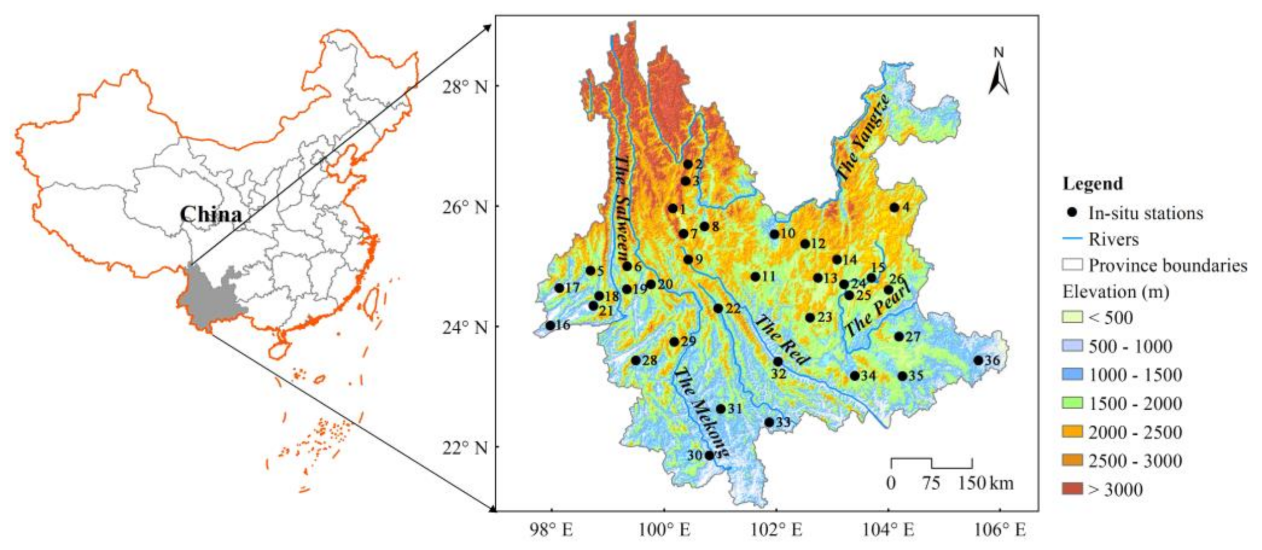
2.1. Study Area

Yunnan province is located in the southwestern region of China, which has an area of approximately 394,000 km2 (21°08′–29°15′ N, 97°31′–106°11′ E) (shown in Figure 1). The climate belongs to the subtropical plateau monsoon and is characterized by distinct dry and wet seasons [50]. Accordingly, precipitation falls during the monsoon season (May–October), accounting for 85% of the total annual precipitation (approximately 1100 mm) [51]. The elevation varies from 6740 to 76 m and decreases from the northwest to the southeast. The mean annual temperature ranges from 5.52 to 23.88 °C, and the mean annual precipitation varies from 560 to 2300 mm [52]. There are many large rivers, such as the Salween, Mekong, Red, Yangtze, and Pearl River, flowing through or originating from this area, which is also an important ecological defense construction area in China. However, increasingly frequent droughts have caused huge socioeconomic losses over the past two decades [52,53]. For example, a record-breaking and persistent drought hit Yunnan from autumn 2009 to spring 2010, resulting in 7.57 million residents suffered from a lack of drinking water. Approximately 21,741 km2 of crops planted in autumn and winter were affected by drought, and the direct agricultural loss exceeded RMB 20 billion [52]. Therefore, SM data derived from multi-sources with fine resolution are necessary for regional drought monitoring.

2.2. Data

2.2.1. SM Data

The SMAP satellite was launched in 2015, carrying an L-band radiometer and radar (non-imaging SAR), which is devoted to providing a global surface (0–5 cm) volumetric SM with a spatial resolution of 36, 9, and 3 km at local overpass times of 06:00 AM (descending orbit) and 06:00 PM (ascending orbits), respectively. Unfortunately, owing to the failure of the radar, only SM from the radiometer is available [54]. The SM data used here was, “SMAP L3 Radiometer Global Daily 36 km EASE-Grid Soil Moisture, Version 7 (L3SMP)”. The L3SMP SM at ascending and descending modes were averaged to obtain daily SM. The L3SMP data were collected from January 2016 to December 2020.
ERA5-Land, a reanalysis dataset released by the European Center for Medium-Range Weather Forecasts (ECMWF), was produced by replaying the land component of the ERA5 data and combining model data with global observations using laws of physics [18]. ERA5-Land includes four layers of SM estimates including 0–7, 7–28, 28–100, and 100–289 cm, which have been available from 1950 to present with a spatial resolution of 0.1° × 0.1° and an hourly temporal resolution. The SM estimate of the top layer (0–7 cm) was used in the current study.
GLDAS generates optimal fields of land surface states by combining satellite data and ground data and utilizing sophisticated land surface modeling and data assimilation methods [17]. GLDAS runs multiple surface models, such as Noah, Mosaic, Community land, and variable infiltration capacity. We obtained the SM estimates from the GLDAS-2.1 Noah model (hereafter GLDAS) with a 0.25° × 0.25° and 3-hourly/monthly resolutions. The GLDAS provides four-layer SM estimates, including 0–10, 10–40, 40–100 and 100–200 cm; the SM estimate at a depth of 0–10 cm was used in the current study.
In situ SM data were collected from 36 automatic measurement stations in Yunnan province (Figure 1), which were obtained from the Yunnan Meteorological Service. These stations provide hourly SM values at different soil depths. In order to match the satellite and modeled SM products, in situ SM data at soil depths of 0–10 cm were used and the time intervals were resampled into monthly average values.

2.2.2. Auxiliary Data

Four Terra Moderate Resolution Imaging Spectroradiometer (MODIS) products were used here, including the monthly normalized difference vegetation index (NDVI) (MOD13A2) product, 8-day land surface temperature (LST) product (MOD11A1), 8-day surface reflectance product (MOD09A1), and yearly land cover type product (MCD12Q1). For LST, the daytime and nighttime LSTs were averaged to obtain daily SM. The surface reflectance product was used to calculate the surface albedo [55]. The outliers of surface reflectance, LST, and NDVI were first eliminated based on the quality flag. Furthermore, null values were interpolated using the Savitzky–Golay (S–G) filter [56]. The land cover type product was utilized here to identify the pixels classified as water bodies and ice/snow. The pixels classified as water and ice/snow were excluded in the analysis. In addition, elevation data with a spatial resolution of 90 m was obtained from the Shuttle Radar Topography Mission (SRTM) [57]. Soil texture is defined as the content of clay, silt, and sand per unit volume of soil mass, which were acquired from the Harmonized World Soil Database (HWSD) [58]. In addition to the above data, precipitation data were adopted to assist the intercomparison of downscaled SM data. The Climate Hazards Group Infrared Precipitation with Stations (CHIRPS) is a 40-year (from 1981 to present) rainfall dataset, which covers most regions of the world (50°S–50°N) [59]. Here, the 0.05° × 0.05° CHIRPS monthly precipitation datasets were used from 2016 to 2020.

2.2.3. Data Preprocessing
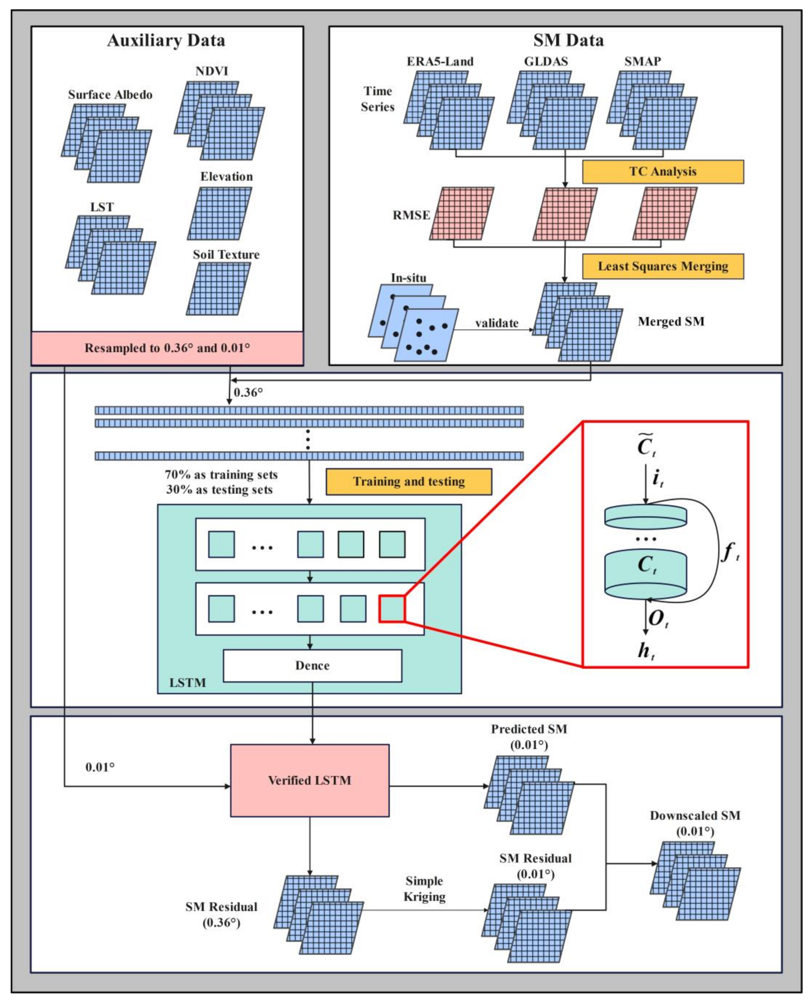
Table 1 lists the SM and auxiliary data used in this study. As the SM and auxiliary data adopted have different resolutions, we established a unified standard for data preprocessing. The georeference of all grid data were set as GCS-WGS-1984. SMAP, ERA-land and GLDAS SM data were resampled to a spatial resolution of 0.36° using the nearest neighbor method. All SM data were averaged to the temporal resolution of a month. The units of all SM data were volume water content (m3/m3). MODIS products were reprojected to the GCS-WGS-1984 coordinate system using the MODIS Reprojection Tool. NDVI, LST, surface albedo, elevation and soil texture were resampled to 0.36° and 0.01°, respectively. In addition, the monthly LST and surface albedo were generated by using the weighted temporal average based on the 8-day LST and 8-day surface albedo in a one month window, respectively. To facilitate comparison, a common period of record from January 2016 to December 2020 was used for all datasets.

3. Methodology

We proposed a hybrid approach combining the TC and LSTM, which was designed to generate a high-quality SM dataset from satellite and modeled data. Figure 2 shows the flowchart of the hybrid approach. This approach includes two steps: (1) SM merging. SMAP, GLDAS, and ERA5-Land SM products are merged by combining the product errors obtained from the TC analysis and the least-squares framework in every pixel [22]; (2) spatial downscaling. The idea was to establish a statistical relationship between the low spatial resolution SM data and environmental variables using LSTM, and then input high spatial resolution environmental variables into verified LSTM to obtain the downscaled SM [44]. The specific process of downscaling can be described as follows:
  • The relationship between the environmental variables and the SM data at a low spatial resolution (0.36°) was established using the LSTM network.
    S M o = f L S T M L S T ,   N D V I ,   s u r f a c e   a l b e d o , e l e v a t i o n , s o i l   t e x t u r e + ε
    where S M o denotes original SM data, f L S T M is a nonlinear function by establishing a relationship between the variables and S M o , and ε is residual, which represents the amount of SM that could not be predicted by LSTM.
  • The LSTM network established in step (Ⅰ) and the variables at 0.36° scale were applied to predict SM ( S M L S T M L ). By subtracting the predictive values from S M o , the residuals at the 0.36° scale were obtained.
    ε = S M o S M L S T M L
  • The residuals ( ε ) were spatially interpolated to form residual maps at a 0.01° resolution ( ε k ) using the simple Kriging technique.
    ε k = i = 1 n λ i ε i
    where λ i are Kriging weights, and ε i is the residual at location i.
  • High spatial resolution variables were entered into the LSTM network established in step (Ⅰ), and a predicted SM of 0.01° resolution ( S M L S T M H ) was achieved.
  • The final downscaled SM ( S M F i n a l ) were obtained by adding the residual term to the predicted SM.
    S M F i n a l = S M L S T M H + ε k
Figure 2. SM merging and downscaling based on the TC-LSTM model.
Remotesensing 14 01744 g002

3.1. TC Analysis

TC [27] is a statistical method used for estimating the random error variance of three datasets required with independent errors [60]. A commonly used error model in the TC approach has the following form:
S M i = S M i + ε i = α i + β i T + ε i ,
where S M i i ϵ 1 ,   2 ,   3 is the value from the three collocated SM datasets linearly related to T, which represents the actual SM value, with random errors ε i , β i , and α i as the bias and scale factors.
We assumed that the errors from independent datasets had zero mean E ε i = 0 , and they were uncorrelated with each other C o v ε i , ε j = 0 , i j and t C o v ε i , T = 0 . Therefore, the covariances between the different SM datasets are expressed as follows:
C i j = C o v S M i , S M j = β i β j σ T 2 ,   i j β i 2 σ T 2 + σ ε i 2 ,   i = j
where σ ε i 2 = V a r ε i . Because the number of unknowns (seven) is greater than that of C (six), there is no unique solution to the equations mentioned above. To solve this problem, a new variable is defined as θ i = β i σ T . Therefore, Equation (6) can be represented by
C i j = θ i θ j ,   i j θ i 2 + σ ε i 2 ,   i = j
The problem can be solved by using six equations and six variables. The RMSE σ ε i was obtained as follows:
σ ε = C 11 C 12 C 13 C 23 C 22 C 12 C 23 C 13 C 33 C 13 C 23 C 12 .
Another extended TC approach was introduced to investigate the correlation with an unknown true SM [61]. β i can be written as:
β i = R T , S M i C i i σ T ,
where R T , S M i is the correlation coefficient between and T and S M i . From Equations (6) and (8), the correlations of the SM data are obtained:
R T , S M = ± C 12 C 13 C 11 C 23 s i g n C 13 C 23 C 12 C 23 C 22 C 13 s i g n C 12 C 23 C 13 C 23 C 33 C 12   ,
which provides important information about the collocation datasets.

3.2. Merging Scheme

It is advantageous to merge different SM products to combine the merits of multi-source SM data and minimize random errors. The least squares method is an evaluation theory and has been used in many studies since it was originally published in 1809 by Gauss [62]. The desired SM value of the merged data can be expressed as [22]:
S M A v e r = w 1 S M 1 + w 2 S M 2 + w 3 S M 3 ,
where w 1 , w 2 , and w 3 represent the weights of three SM products: S M 1 , S M 2 , and S M 3 , respectively. To obtain unbiased fusion data, the following is required:
w 1 + w 2 + w 3 = 1 .
Based on the above constraints, our goal was to express the weights as a function of the mean square error of the three datasets. Therefore, the mean square errors of the merged data can be expressed as:
σ m 2 = w 1 2 σ 1 2 + w 2 2 σ 2 2 + w 3 2 σ 3 2 ,
which is:
σ m 2 = w 1 2 σ 1 2 + 1 w 1 w 3 2 σ 2 2 + w 3 2 σ 3 2 .
Setting σ m 2 w 1 = 0 and σ m 2 w 3 = 0 in Equation (15) and solving for w 1 , w 2 , and w 3 , we obtain the following:
W 1 = σ 2 2 σ 3 2 σ 1 2 σ 2 2 + σ 1 2 σ 3 2 + σ 2 2 σ 3 2 ,
W 2 = σ 1 2 σ 3 2 σ 1 2 σ 2 2 + σ 1 2 σ 3 2 + σ 2 2 σ 3 2 ,
W 3 = σ 1 2 σ 2 2 σ 1 2 σ 2 2 + σ 1 2 σ 3 2 + σ 2 2 σ 3 2 .
The solution is intuitive because the weights are proportional to the errors of the other two estimates.

3.3. LSTM

LSTM was proposed to solve the problem of exploding and vanishing gradients [63]. A common LSTM unit consists of several memory cells, each of which contains three gates (input, output, and forget). These gates control the information that is discarded and retained from the previous moment; therefore, LSTM has an inherent advantage in extracting contextual information, such as temporal characteristics [64]. A memory cell of the LSTM framework can be expressed as
i t = σ W i h t 1 , x t + b i ,
f t = σ W f h t 1 , x t + b f ,
o t = σ W o h t 1 , x t + b o ,
C ˜ t = tanh W c h t 1 , x t + b c ,
C t = f t C t 1 + i t C ˜ t ,
h t = o t tanh C t ,
where i t , f t , o t , and C ˜ t represent the three gates and an intermediate state that are input, forget, output gates, and candidate state, respectively, which are the output vectors of the sigmoid layer with a range of 0 to 1. C t and C t 1 indicate the cell states delivering information in the current and last moments, respectively, while x t indicates the input information at the current moment. h t and h t 1 carry the output information of the cells at the current and last moments, respectively. W i , W f , W o , and W c are the parameter matrices to be trained, and b i , b f , b o , and b c are bias items to be trained. In addition, tanh is defined as a hyperbolic tangent function in mathematics. First, Equations (19)–(21) are used to determine whether the information from the last moment ( h t 1 ) and that from this moment ( x t ) is to be retained or not. Then, Equation (23) is used to calculate the result of this moment and pass it to the next moment. More details about LSTM can be found in previous studies [65,66,67].
Connecting such multiple cells to form more complex structures can solve practical sequence problems. In this study, a two-layer LSTM structure with 80 and 100 cells was used to fit the relationship between the SM data and explanatory variables (LST, NDVI, surface albedo, elevation, and soil texture), which was accomplished using the TensorFlow package of Python. In addition, modeling processes often have the problem of overfitting, which depends on the model structure when the samples are the same. Generally, it can be solved by utilizing the dropout function and the early stopping method [65]. Therefore, in this study, a dropout layer with a parameter of 0.2 was added after each layer of LSTM to discard 20% of the data, in order to avoid overfitting. Additionally, some other parameters also needed to be set. For example, the maximum number of iterations was 200, and the optimizer used was Adam, whose initial learning rate and loss function were set as 0.001 and mean squared error, respectively.

3.4. Evaluation Metrics

The accuracy of satellite, modeled, merged, and downscaled SM data were evaluated using in situ data as the reference. In this study, four metrics consisting of the correlation coefficient (R), root mean square error (RMSE), unbiased root mean square error (ubRMSE), and bias were used [68]. Detailed information on the four metrics is presented in Table 2.

4. Results

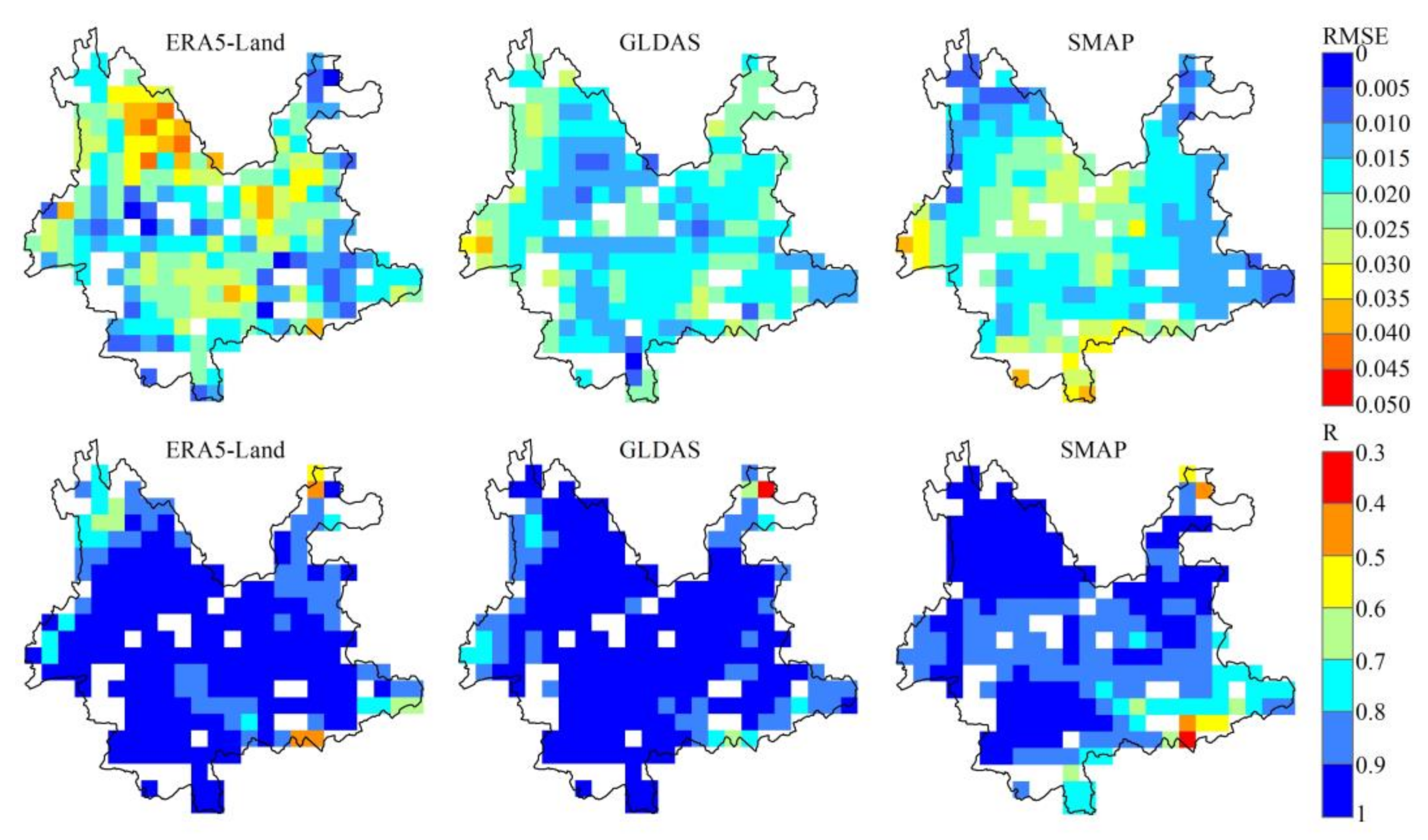
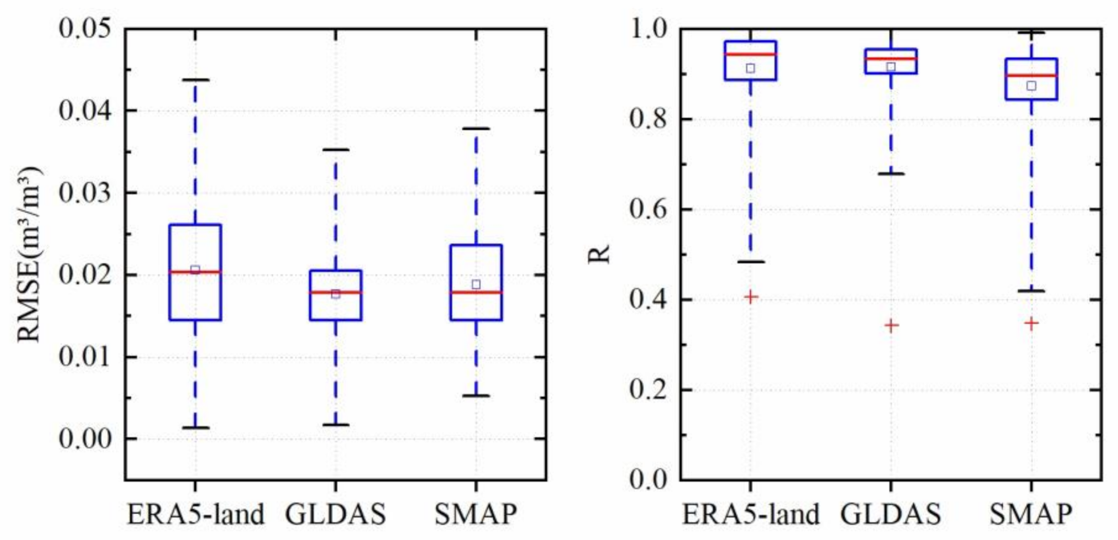
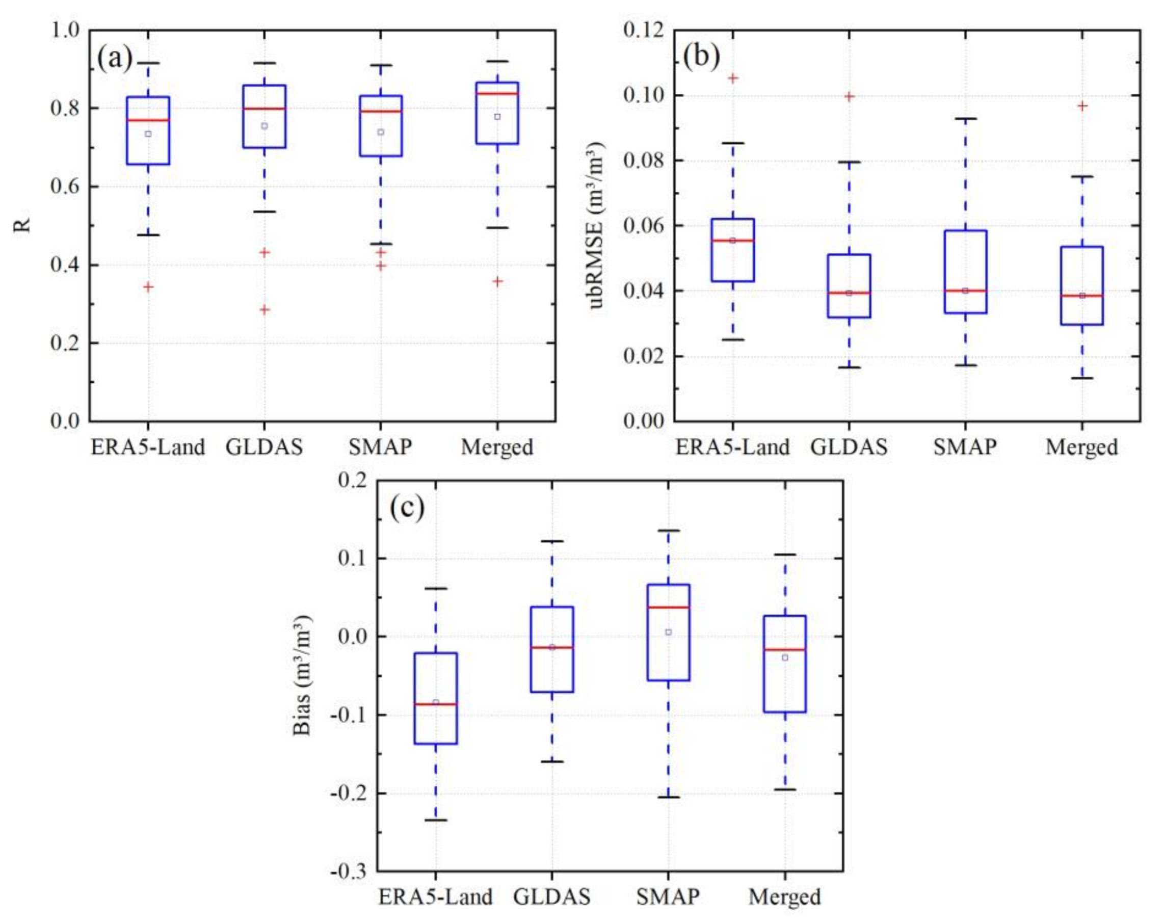
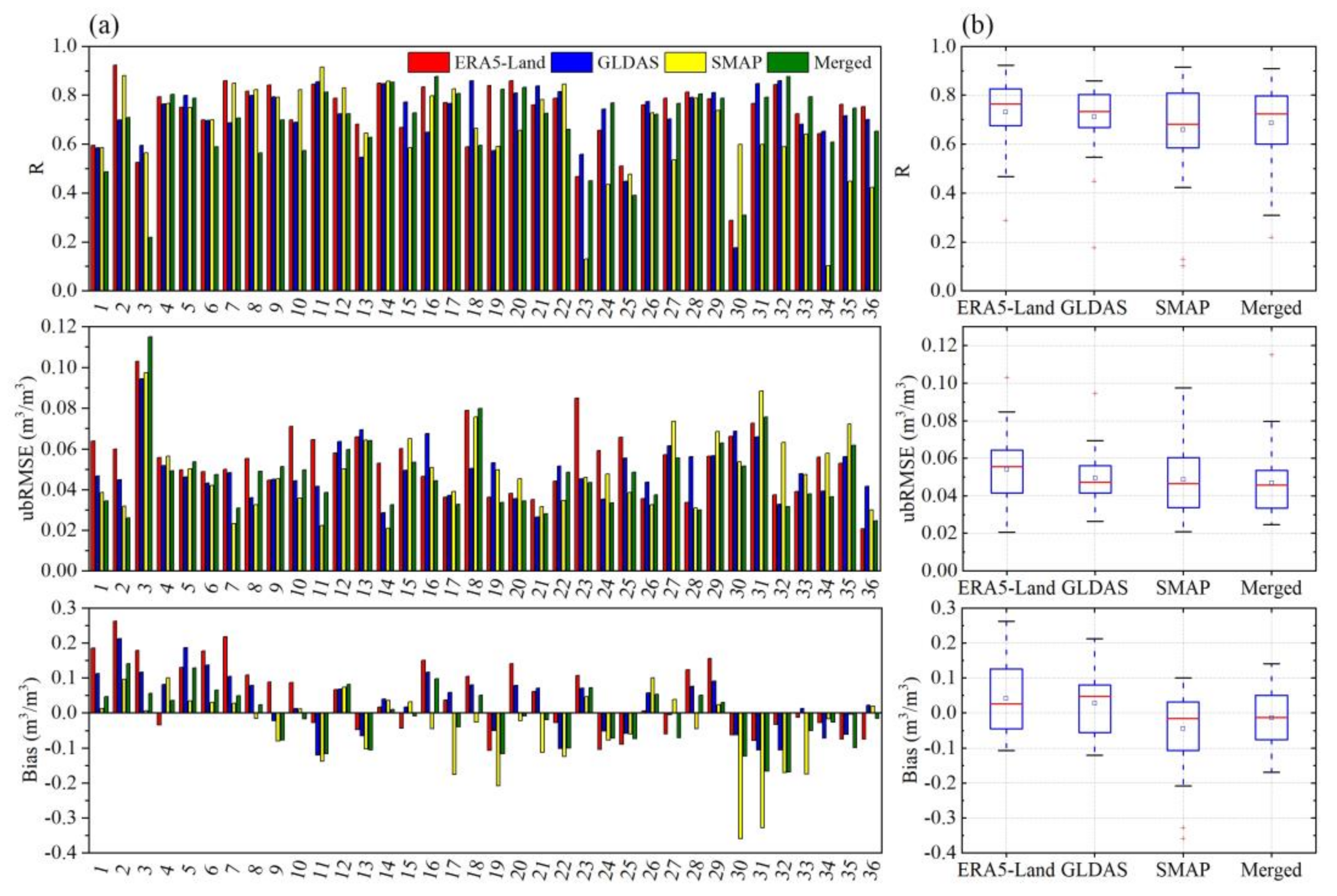
4.1. TC-Based Assessment

In this study, a satellite product (SMAP) and two modeled products (ERA5-Land and GLDAS) were used in one TC triplet. The TC-based error estimates required three collocated SM datasets that were significantly correlated [21,22]. We evaluated the cross correlation of ERA5-Land, GLDAS, and SMAP using Pearson correlation coefficients (Figure S1). The results showed significant correlations among ERA5-Land, GLDAS, and SMAP over most areas (p < 0.05), suggesting a strong mutual linear relationship among the three SM products. Figure 3 displays the spatial distribution of the random error variance and correlation for ERA5-Land, GLDAS, and SMAP products based on TC analysis. The unresolved pixels, due to violation of assumptions in the TC analysis were excluded, which accounted for approximately 14% of the total pixels in the study area. The spatial pattern of the random error variance varied among the different SM products. For example, ERA5-Land had relatively high errors in the northwest region, where the topography is complex. In the central region, the error of the GLDAS was generally relatively low and spatially homogeneous. In addition, SMAP performed better in the northwest and southeast regions. In terms of the correlation, all products showed a high correlation (above 0.8) with the unknown truth in most areas, except in the northwest and southeast regions.
Figure 4 shows a summary of the correlation and random error variance for ERA5-Land, GLDAS, and SMAP products based on TC analysis. At the regional scale, GLDAS showed the highest average correlation with the unknown truth (0.92), followed by ERA-land (0.91) and SMAP (0.88). The error variance was slightly different from the correlation, with the lowest averaged RMSE for GLDAS (0.018 m3/m3), and slightly larger RMSE for SMAP (0.019 m3/m3) and ERA-land (0.021 m3/m3). It can be seen that the GLDAS has the best performance with high correlation and relatively low errors among the three products. This is consistent with previous work reporting that GLDAS outperformed SMAP and ERA5 in root zone SM estimates on a global scale [30].

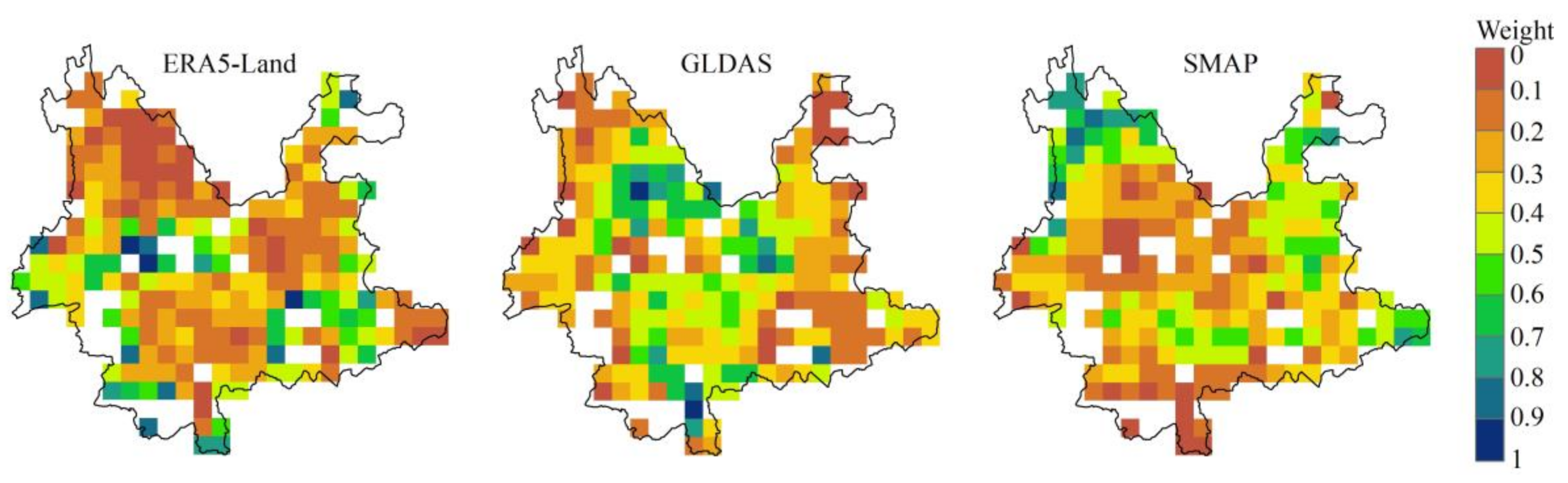
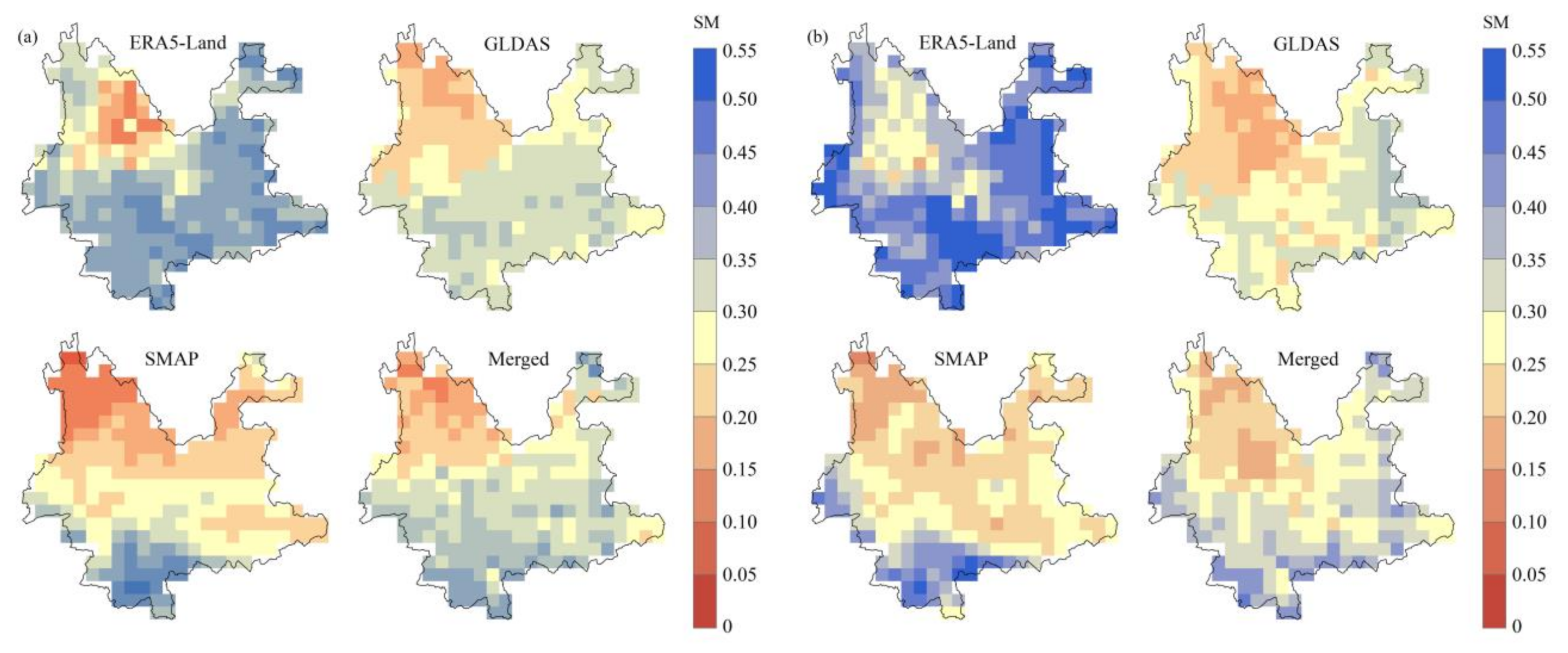
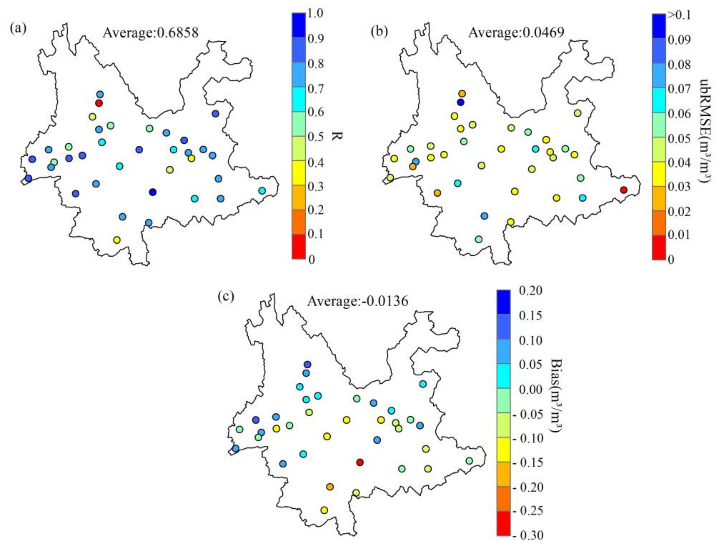
4.2. SM Merging Based on TC

Figure 5 shows the merging weights of ERA5-Land, GLDAS, and SMAP. The spatial distribution of the merging weights was consistent with the random error variance (Figure 3), specifically, the pixels with high RMSE had low weights, while the pixels with low RMSE were assigned high weights. Model-based SM is strongly dependent on externally supplied meteorological forcing data, which can significantly influence SM simulation [69]. In the northwest region with the complex terrain, input precipitation is less reliable, which may explain the less accuracy and low weight of ERA5-Land and GLDAS. In addition, SMAP SM is sensitive to vegetation, higher vegetation intensity will reduce the quality of SM [70]. For instance, the SMAP was assigned low weights in the western and southern regions, which attributed to dense vegetation. Overall, GLDAS had the highest space-averaged weight (0.36), followed by SMAP (0.33) and ERA5-Land (0.31). It can be seen that the merging weights varied among the parent products and showed spatial variability. It is worth noting that the blank areas in the maps, due to violation assumptions in TC analysis, were merged using a simple arithmetic average to increase the coverage of the merged product.
Figure 6 shows the spatial distributions of the SM for the three parent products and the merged product using TC analysis; the SM levels in January and June 2019 were used as examples. Generally, the three parent datasets showed distinct spatial differences. For example, ERA5-Land showed much wetter conditions in the southern and eastern regions than GLDAS and SMAP. In theory, the merged data should integrate the characteristics of the three parent products and minimize the errors of the parent products. Although distinct spatial variation was observed in parent products, the merged SM dataset had similar patterns of wet and dry distributions to these parent products, which presented lower SM in the northwestern region, and a general increase in the eastern and southern parts of Yunnan province.
To evaluate the accuracy of these parent products and the merged products, we compared the SM estimates with the in situ observations. Figure 7 shows box plots of the validation results of different SM datasets at the in situ stations. The median R-values for ERA5-Land, GLDAS, SMAP, and the merged datasets were 0.77, 0.80, 0.79, and 0.84, respectively. The medians of ubRMSE were 0.055, 0.039, 0.040, and 0.039 m3/m3, and the medians of bias were −0.086, −0.014, 0.038, and −0.017 m3/m3 for ERA5-Land, GLDAS, SMAP, and merged datasets, respectively. Among the three parent products, GLDAS had the best performance with the lowest median of ubRMSE and bias and the highest median of correlation, followed by SMAP and ERA5-Land. These results were consistent with those of the TC-based assessment (Figure 4). The highest median R-value and lowest median of ubRMSE from the merged datasets compared with the in situ observations were very encouraging. We found that the median bias of the merged datasets was lower than that of ERA5-Land and SMAP, but the median bias for GLDAS was slightly better than that for the merged datasets. This may be attributed to the parent products having large biases (a median bias of −0.086 for ERA5-Land) compared to in situ observations; thus, there may be limited improvements in the merged product. Overall, the merged dataset showed its advantages integrated from satellite and modeled products, indicating that the TC-based merging method can be used to generate high-quality, spatiotemporal continuous SM data from satellite and modeled SM data.

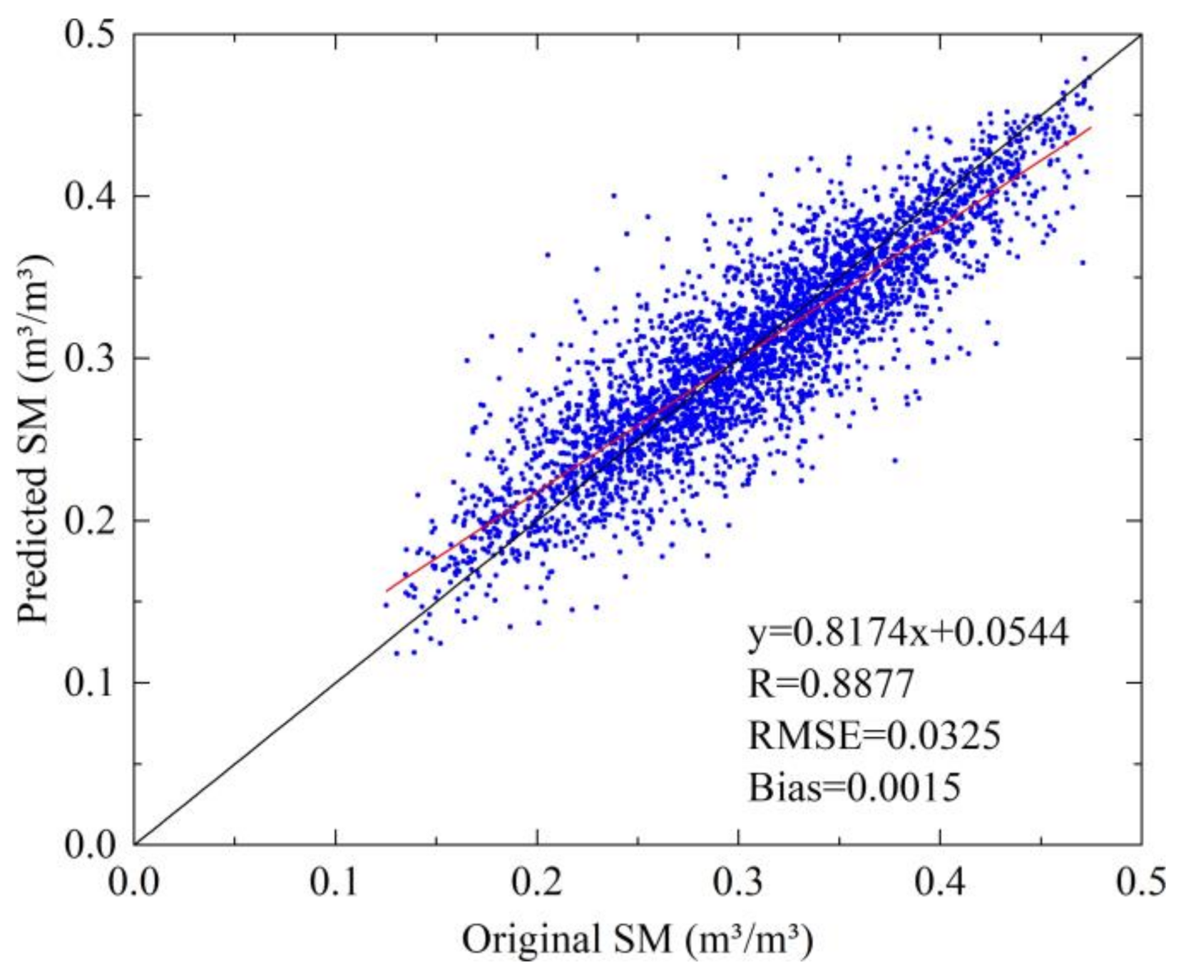
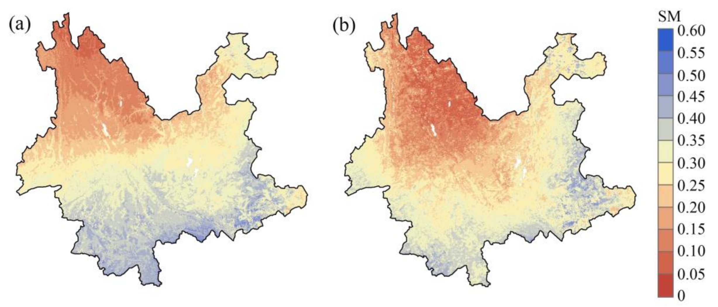
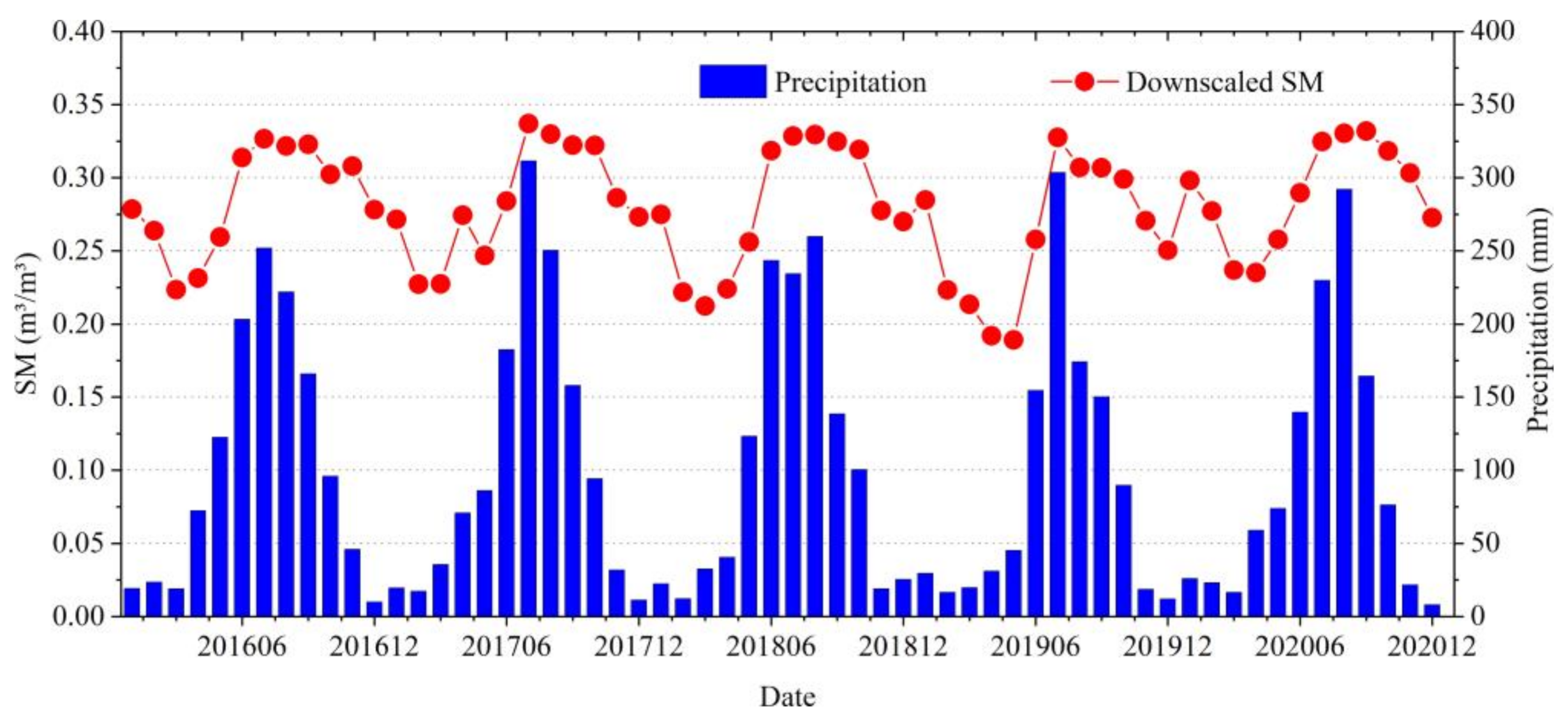
4.3. SM Downscaling Based on LSTM

The downscaling method assumed that the regression relationship between the SM data and auxiliary environmental variables (elevation, LST, NDVI, surface albedo, and soil texture) at a coarse spatial scale (0.36°) was equally effective at a fine scale (0.01°). The first step was to train and verify the LSTM network using the environmental variables sampled from locations where merged SM data (0.36°) were available. In the training process, 70% of the total data were selected randomly as the training set and the other 30% as the verification set [71]. Figure 8 illustrates the scatter plot showing the merged SM and predicted test dataset by fitting the merged SM and environmental variables based on the LSTM network. The LSTM revealed a significant relationship between the merged SM data and environmental variables. There is very good agreement between the original and predicted SM values (R = 0.8877, RMSE = 0.0325 m3/m3, and bias = 0.0015 m3/m3). Additionally, the slope and intercept of the regression linear equation were 0.82 and 0.05, respectively, indicating that the predicted SM values were close to the merged SM, and the overestimation and underestimation values were not significant. In the next step, the verified LSTM network was applied to the auxiliary environmental variables at 0.01° resolution to obtain high-resolution SM data over the period from January 2016 to December 2020. The spatial patterns of the downscaled SM in January and June 2019, are shown in Figure 9. The downscaled SM not only had a similar distribution as the original merged SM data but also captured detailed information on the spatial heterogeneity of SM compared to the original merged SM data (Figure 6).
The downscaled SM data were validated using the observation records of 36 in situ sites (Figure 10). The results indicated that the downscaled SM data had a high correlation with in situ data almost everywhere across Yunnan province, except for a few individual sites with slightly low correlation in the central and southern regions. There were similar patterns in ubRMSE and bias, which have relatively small values in most sites of Yunnan province and slightly larger values at some sporadic points. Generally, the downscaled SM data agreed well with the in situ observations. The mean and median values of R, ubRMSE, and bias were 0.6858 and 0.7244; 0.0469 m3/m3 and 0.0459 m3/m3; and −0.0136 m3/m3 and −0.0126 m3/m3, respectively. It is worthy to note that the validation results are inevitably affected by the limited number of in situ stations, the spatial scale differences between the in situ networks and downscaled data, and the differences in the surface soil depths of SM products [72]. Figure 11 and Figure S2 show that the temporal variation of the downscaled SM agreed well with the precipitation data, both at regional and station scales. The variations between dry and wet seasons and the effect of precipitation can be well reflected by the downscaled SM data. In addition, the downscaled SM data reflected the severe drought conditions of Yunnan province in 2019. The results demonstrated that the downscaled SM could reflect actual SM dynamics.
The downscaled SM of the merged product was also compared with those downscaled SM levels from ERA5-Land, GLDAS, and SMAP (Figure 12). It was shown that the performances of all downscaled products varied over different stations. At most stations, the downscaled SM of the merged product outperformed other downscaled SM products with lower ubRMSE and bias. At the regional scale, the downscaled SM of the merged product showed a higher median R (0.7244) than that of SMAP (0.6814), but a lower median R than that of ERA5-Land (0.7647) and GLDAS (0.7332). The median ubRMSE of the downscaled SM of the merged product was 0.0459 m3/m3, which was slightly better than that of ERA5-Land (0.0556 m3/m3), GLDAS (0.0473 m3/m3), and SMAP (0.0467 m3/m3). In terms of median bias, the lowest absolute value was found for the merged product (−0.0126 m3/m3), followed by SMAP (−0.0159 m3/m3), ERA5-Land (0.0267 m3/m3), and GLDAS (0.0483 m3/m3). The comparison results indicated the downscaled SM of the merged product had better performance, including the acceptable R, lowest ubRMSE, and bias values among all the evaluated products. It is worth noting that the proposed downscaling method contained several assumptions and possible uncertainties from the auxiliary data; however, the validation results implied that the fusion of satellite- and model-based SM data would result in better downscaling accuracy.

5. Discussion

The uncertainties of ERA5-Land, GLDAS, and SMAP were first evaluated by a TC analysis. The results showed that GLDAS outperformed SMAP and ERA5-Land (Figure 4). Similar results were obtained from direct comparisons with in situ observations (Figure 7), indicating that the TC analysis was reasonable for the comparison and evaluation of satellite or modeled SM datasets in data-scarce areas. As shown in Figure 7, the TC-based merged dataset showed its advantages integrated from satellite and modeled products. In the TC analysis, the errors of SM datasets are assumed to be mutually independent and orthogonal to the truth [73]. The simultaneous use of both model-based products (ERA5-Land and GLDAS) may imperil the mutual error independence results underlying the application of TC analysis [74]. Therefore, a triple combination of an active-based product (active SM product of the European Space Agency Climate Change Initiative (v06.1), CCI-active) [75], a passive-based product (SMAP), and a model-based product (ERA5-Land) was also applied here to calculate TC-based metrics. Figure S3 shows box plots of the validation results of different SM datasets at the in situ stations. The results also confirmed the merged SM data based on TC was superior to their parent products, which proves that TC-based merging was a reliable way to blend satellite and model-based SM products [19,21,22,25,31].
In theory, the TC-based merged data should outperform simple averaging data. However, this was not the case in some studies [19,22,25]. Figure S4 shows a comparison between the two SM datasets obtained by TC and simple arithmetic mean merging methods. For triplet A (SMAP, ERA5-Land, and GLDAS), it was found that the TC-based merged data were only slightly better than the simple averaging data in terms of R and bias. The reason could be that the differences among the three parent products were small or the weights of the three parent products were approximately equal [19]. However, for triplet B (CCI-active, SMAP, and ERA5-Land), the TC-based merged data were preferred over simple averaging data, because it can provide optimal weights and generate a better merged product in areas where the parent products have large differences (Figure S3) [19]. In addition, it should be noted that only 36 in situ stations were used for comparison and validation. The validated results were affected by the representativeness errors of the limited stations.
The merging method based on TC analysis could be further improved in the following aspects. It only allowed the input of three parent products, which resulted in the merged result of TC varying with a change in choice of the three inputs. Theoretically, the more input of SM products, the better the merged SM data that may be obtained. To overcome this limitation, Pan et al. (2015) proposed an improved TC method that allowed the input of more than three products when evaluating them [76]. In addition, a three-cornered hat is an alternative used for estimating the error variance of more than three products [15,77]. Moreover, the TC-based merging method assumed that the errors of the data in the time dimension were constant. In fact, the errors in SM data exhibit significant temporal variations with time changes [78]. A constant weight for the entire period may not reflect the error characteristics. Therefore, spatial and temporal non-stationary errors should be considered to improve the TC merging skill [26,79].
Analysis of the importance of different environmental variables in the SM downscaling process can help understand the mechanism of the impact of surface variables on SM [10,38]. In order to analyze the importance of input variables (LST, NDVI, surface albedo, elevation, and soil texture) in the downscaling process, we conducted a leave-one-out approach in which one of the input environmental variables was removed and downscaling was accomplished [36]. Figure S5 shows the validation results for the different input schemes. It was found that elevation, NDVI, and surface albedo were the three most important variables in SM downscaling. The local topography is important in determining SM over regions with sharp elevation fluctuations [8,37]. NDVI and surface albedo also exhibited high importance in SM downscaling due to their ability to reflect vegetation status and surface energy exchange [80]. LST was identified as the most important variable in some previous studies [10,38]; however, our results indicated LST showed relatively less influence on the downscaling results. This may be attributed to poor quality of MODIS LST due to cloud contamination in the study area.
ML was widely used to downscale SM data in case studies [10,36,37,38,39,45]. The performance of ML in SM spatial downscaling varies with the algorithms and regions [37]. However, traditional ML algorithms cannot consider the feature abstraction of sequence data and contextual correlation on the time axis. As a class of recurrent neural networks (RNNs), the LSTM network can consider contextual information of the original data and would theoretically be more suitable for modeling time-series data [49,81]. For example, it was used in rainfall–runoff modeling [82], terrestrial water storage reconstructing [83], drought forecasting [84], and rice yield predicting [71]. The SM downscaling based on LSTM had a satisfactory performance in this study (Figure 8 and Figure 10), although the accuracy of downscaled results was associated with the uncertainties from input remotely sensed products, the effect of the scale, and the accuracy and representativeness of in situ observations [44]. Our results showed that LSTM had broad application prospects in SM downscaling and prediction [85]. However, LSTM is designed to process sequence data, it can only obtain a temporal relationship. We also recommended CNNs in subsequent research because they can capture the spatial features from three-dimensional images [86,87]. Furthermore, the convolutional LSTM (ConvLSTM) combines the capabilities of CNN and LSTM, which not only account for the temporal relationship, but also extract spatial features through the convolution layer and are expected to further improve the SM predictive performance [48,88,89].

6. Conclusions

This study presented a hybrid TC-LSTM approach to generate a high-quality SM dataset with a 0.01 resolution and a monthly temporal resolution based on satellite- and model-based data. For the evaluation of the SMAP, GLDAS, and ERA5-Land SM products, similar results were obtained from direct comparisons with in situ observations and TC error estimation, indicating that the TC analysis was reasonable for the comparison and evaluation of satellite and model-based SM products. In addition, TC-based merging was superior to simple arithmetic average merging when the parent products had large differences. The downscaled SM of TC-based merged product had better performance, including the acceptable R, lowest ubRMSE, and bias values among all of the evaluated products, implying that the fusion of satellite and model-based SM data would result in better downscaling accuracy. The downscaled merged SM data obtained using the LSTM not only improved the spatial resolution of the SM data and captured the spatial heterogeneity and dynamics of SM but also yielded satisfactory results with a median value of R (0.7244), ubRMSE (0.0459 m3/m3), and bias (−0.0126 m3/m3) when validated with in situ observations. Overall, the proposed approach in this study had no strict boundary conditions and, thus, had better universality in various climate conditions. It could generate a SM dataset with a fine resolution and reliable accuracy for wide hydrometeorological applications.

Supplementary Materials

The following supporting information can be downloaded at: https://0-www-mdpi-com.brum.beds.ac.uk/article/10.3390/rs14071744/s1, Figure S1: The spatial distribution of the cross-correlation of three SM products, Figure S2: Temporal variations of downscaled SM and CHIRPS precipitation at representative site, Figure S3: The evaluation of SM datasets using in situ observations for validation, Figure S4: The evaluation of SM datasets merged by TC and simple arithmetic averaging (SAA) for two triplets using in situ observations for validation, Figure S5: Performance evaluation of the downscaling algorithms under different input schemes using in situ observations.

Author Contributions

Conceptualization and methodology, Y.L. and X.J.; software, W.M., Y.W., and J.L.; validation, W.M. and X.J; formal analysis, W.M., C.L., and Y.L.; investigation, W.M., C.L., and M.Z.; resources, M.Z. and Y.L.; data curation, W.M. and M.Z.; writing—original draft preparation, W.M.; writing—review and editing, Y.L., W.M., and X.J; visualization, Y.W. and J.L.; supervision, Y.L. and X.J.; project administration, Y.L.; funding acquisition, Y.L. All authors have read and agreed to the published version of the manuscript.

Funding

This research was funded by the National Natural Science Foundation of China (grant number 42067033) and the Applied Basic Research Programs of Yunnan province (grant number 202001BB050073).

Institutional Review Board Statement

Not applicable.

Informed Consent Statement

Not applicable.

Data Availability Statement

The SMAP product can be obtained at https://nsidc.org/data/SPL3SMP/ (accessed on 24 November 2021). ERA5-Land product is available at https://cds.climate.copernicus.eu/ (accessed on 26 July 2021). GLDAS product can be accessed at https://ldas.gsfc.nasa.gov/data/ (accessed on 17 November 2021). CCI-active product can be obtained at https://www.esa-soilmoisture-cci.org/ (accessed on 21 November 2021). MODIS data can be accessed at https://search.earthdata.nasa.gov/ (accessed on 31 October 2021). CHIRPS precipitation data is available at https://data.chc.ucsb.edu/products/ (accessed on 26 November 2021). SRTM can be obtained at https://srtm.csi.cgiar.org/ (accessed on 12 August 2021). HWSD can be obtained at https://www.fao.org/soilsportal/ (accessed on 12 August 2021).

Acknowledgments

The authors would like to thank the reviewers and the managing editor for their comments and suggestions, which improved this paper.

Conflicts of Interest

The authors declare no conflict of interest.

References

  1. Babaeian, E.; Sadeghi, M.; Jones, S.B.; Montzka, C.; Vereecken, H.; Tuller, M. Ground, Proximal, and Satellite Remote Sensing of Soil Moisture. Rev. Geophys. 2019, 57, 530–616. [Google Scholar] [CrossRef] [Green Version]
  2. Song, P.L.; Zhang, Y.Q.; Tian, J. Improving Surface Soil Moisture Estimates in Humid Regions by an Enhanced Remote Sensing Technique. Geophys. Res. Lett. 2021, 48, 10. [Google Scholar] [CrossRef]
  3. Sehgal, V.; Gaur, N.; Mohanty, B.P. Global Flash Drought Monitoring Using Surface Soil Moisture. Water Resour. Res. 2021, 57, 25. [Google Scholar] [CrossRef]
  4. Brocca, L.; Melone, F.; Moramarco, T.; Wagner, W.; Naeimi, V.; Bartalis, Z.; Hasenauer, S. Improving runoff prediction through the assimilation of the ASCAT soil moisture product. Hydrol. Earth Syst. Sci. 2010, 14, 1881–1893. [Google Scholar] [CrossRef] [Green Version]
  5. Rigden, A.J.; Mueller, N.D.; Holbrook, N.M.; Pillai, N.; Huybers, P. Combined influence of soil moisture and atmospheric evaporative demand is important for accurately predicting US maize yields. Nat. Food 2020, 1, 9. [Google Scholar] [CrossRef] [Green Version]
  6. Trugman, A.T.; Medvigy, D.; Mankin, J.S.; Anderegg, W.R.L. Soil Moisture Stress as a Major Driver of Carbon Cycle Uncertainty. Geophys. Res. Lett. 2018, 45, 6495–6503. [Google Scholar] [CrossRef]
  7. Dobriyal, P.; Qureshi, A.; Badola, R.; Hussain, S.A. A review of the methods available for estimating soil moisture and its implications for water resource management. J. Hydrol. 2012, 458, 110–117. [Google Scholar] [CrossRef]
  8. Crow, W.T.; Berg, A.A.; Cosh, M.H.; Loew, A.; Mohanty, B.P.; Panciera, R.; de Rosnay, P.; Ryu, D.; Walker, J.P. Upscaling Sparse Ground-Based Soil Moisture Observations for the Validation of Coarse-Resolution Satellite Soil Moisture Products. Rev. Geophys. 2012, 50, 20. [Google Scholar] [CrossRef] [Green Version]
  9. Lekshmi, S.U.S.; Singh, D.N.; Baghini, M.S. A critical review of soil moisture measurement. Measurement 2014, 54, 92–105. [Google Scholar] [CrossRef]
  10. Zhao, W.; Sanchez, N.; Lu, H.; Li, A.N. A spatial downscaling approach for the SMAP passive surface soil moisture product using random forest regression. J. Hydrol. 2018, 563, 1009–1024. [Google Scholar] [CrossRef]
  11. Wagner, W.; Hahn, S.; Kidd, R.; Melzer, T.; Bartalis, Z.; Hasenauer, S.; Figa-Saldana, J.; de Rosnay, P.; Jann, A.; Schneider, S.; et al. The ASCAT Soil Moisture Product: A Review of its Specifications, Validation Results, and Emerging Applications. Meteorol. Z. 2013, 22, 5–33. [Google Scholar] [CrossRef] [Green Version]
  12. Kerr, Y.H.; Waldteufel, P.; Wigneron, J.-P.; Delwart, S.; Cabot, F.; Boutin, J.; Mecklenburg, S. The SMOS Mission: New Tool for Monitoring Key Elements ofthe Global Water Cycle. Proc. IEEE 2010, 98, 666–687. [Google Scholar] [CrossRef] [Green Version]
  13. Chan, S.K.; Bindlish, R.; O’Neill, P.; Jackson, T.; Kerr, Y. Development and assessment of the SMAP enhanced passive soil moisture product. Remote Sens. Environ. 2018, 204, 2539–2542. [Google Scholar] [CrossRef] [PubMed] [Green Version]
  14. Chew, C.; Small, E. Description of the UCAR/CU Soil Moisture Product. Remote Sens. 2020, 12, 1558. [Google Scholar] [CrossRef]
  15. Liu, J.; Chai, L.N.; Dong, J.Z.; Zheng, D.H.; Wigneron, J.P.; Liu, S.M.; Zhou, J.; Xu, T.R.; Yang, S.Q.; Song, Y.Z.; et al. Uncertainty analysis of eleven multisource soil moisture products in the third pole environment based on the three-corned hat method. Remote Sens. Environ. 2021, 255, 20. [Google Scholar] [CrossRef]
  16. Kim, H.; Parinussa, R.; Konings, A.G.; Wagner, W.; Cosh, M.H.; Lakshmi, V.; Zohaib, M.; Choi, M. Global-scale assessment and combination of SMAP with ASCAT (active) and AMSR2 (passive) soil moisture products. Remote Sens. Environ. 2018, 204, 260–275. [Google Scholar] [CrossRef]
  17. Rodell, M.; Houser, P.R.; Jambor, U.; Gottschalck, J.; Mitchell, K.; Meng, C.J.; Arsenault, K.; Cosgrove, B.; Radakovich, J.; Bosilovich, M.; et al. The global land data assimilation system. Bull. Amer. Meteorol. Soc. 2004, 85, 381–394. [Google Scholar] [CrossRef] [Green Version]
  18. Munoz-Sabater, J.; Dutra, E.; Agusti-Panareda, A.; Albergel, C.; Arduini, G.; Balsamo, G.; Boussetta, S.; Choulga, M.; Harrigan, S.; Hersbach, H.; et al. ERA5-Land: A state-of-the-art global reanalysis dataset for land applications. Earth Syst. Sci. Data 2021, 13, 4349–4383. [Google Scholar] [CrossRef]
  19. Peng, J.; Tanguy, M.; Robinson, E.L.; Pinnington, E.; Evans, J.; Ellis, R.; Cooper, E.; Hannaford, J.; Blyth, E.; Dadson, S. Estimation and evaluation of high-resolution soil moisture from merged model and Earth observation data in the Great Britain. Remote Sens. Environ. 2021, 264, 18. [Google Scholar] [CrossRef]
  20. Wu, Z.Y.; Feng, H.H.; He, H.; Zhou, J.H.; Zhang, Y.L. Evaluation of Soil Moisture Climatology and Anomaly Components Derived From ERA5-Land and GLDAS-2.1 in China. Water Resour. Manag. 2021, 35, 629–643. [Google Scholar] [CrossRef]
  21. Gruber, A.; Dorigo, W.A.; Crow, W.; Wagner, W. Triple Collocation-Based Merging of Satellite Soil Moisture Retrievals. IEEE Trans. Geosci. Remote Sens. 2017, 55, 6780–6792. [Google Scholar] [CrossRef]
  22. Yilmaz, M.T.; Crow, W.T.; Anderson, M.C.; Hain, C. An objective methodology for merging satellite- and model-based soil moisture products. Water Resour. Res. 2012, 48, 15. [Google Scholar] [CrossRef]
  23. Liu, Y.Y.; Parinussa, R.M.; Dorigo, W.A.; De Jeu, R.A.M.; Wagner, W.; van Dijk, A.; McCabe, M.F.; Evans, J.P. Developing an improved soil moisture dataset by blending passive and active microwave satellite-based retrievals. Hydrol. Earth Syst. Sci. 2011, 15, 425–436. [Google Scholar] [CrossRef] [Green Version]
  24. Cui, Y.K.; Yang, X.B.; Chen, X.; Fan, W.J.; Zeng, C.; Xiong, W.T.; Hong, Y. A two-step fusion framework for quality improvement of a remotely sensed soil moisture product: A case study for the ECV product over the Tibetan Plateau. J. Hydrol. 2020, 587, 12. [Google Scholar] [CrossRef]
  25. Zhang, N.; Quiring, S.M.; Ford, T.W. Blending Noah, SMOS, and in Situ Soil Moisture Using Multiple Weighting and Sampling Schemes. J. Hydrometeorol. 2021, 22, 1835–1854. [Google Scholar] [CrossRef]
  26. Zhou, J.H.; Crow, W.T.; Wu, Z.Y.; Dong, J.Z.; He, H.; Feng, H.H. A triple collocation-based 2D soil moisture merging methodology considering spatial and temporal non-stationary errors. Remote Sens. Environ. 2021, 263, 16. [Google Scholar] [CrossRef]
  27. Stoffelen, A. Toward the true near-surface wind speed: Error modeling and calibration using triple collocation. J. Geophys. Res.-Oceans 1998, 103, 7755–7766. [Google Scholar] [CrossRef]
  28. Gruber, A.; Su, C.H.; Zwieback, S.; Crowd, W.; Dorigo, W.; Wagner, W. Recent advances in (soil moisture) triple collocation analysis. Int. J. Appl. Earth Obs. Geoinf. 2016, 45, 200–211. [Google Scholar] [CrossRef]
  29. Wu, X.T.; Lu, G.H.; Wu, Z.Y.; He, H.; Scanlon, T.; Dorigo, W. Triple Collocation-Based Assessment of Satellite Soil Moisture Products with In Situ Measurements in China: Understanding the Error Sources. Remote Sens. 2020, 12, 2275. [Google Scholar] [CrossRef]
  30. Xu, L.; Chen, N.C.; Zhang, X.; Moradkhani, H.; Zhang, C.; Hu, C.L. In-situ and triple-collocation based evaluations of eight global root zone soil moisture products. Remote Sens. Environ. 2021, 254, 16. [Google Scholar] [CrossRef]
  31. Mousa, B.G.; Shu, H. Spatial Evaluation and Assimilation of SMAP, SMOS, and ASCAT Satellite Soil Moisture Products Over Africa Using Statistical Techniques. Earth Space Sci. 2020, 7, 16. [Google Scholar] [CrossRef] [Green Version]
  32. Das, N.N.; Entekhabi, D.; Njoku, E.G. An Algorithm for Merging SMAP Radiometer and Radar Data for High-Resolution Soil-Moisture Retrieval. IEEE Trans. Geosci. Remote Sens. 2011, 49, 1504–1512. [Google Scholar] [CrossRef]
  33. Fang, B.; Lakshmi, V.; Bindlish, R.; Jackson, T.J.; Cosh, M.; Basara, J. Passive Microwave Soil Moisture Downscaling Using Vegetation Index and Skin Surface Temperature. Vadose Zone J. 2013, 12, 1. [Google Scholar] [CrossRef]
  34. Kim, J.; Hogue, T.S. Improving Spatial Soil Moisture Representation Through Integration of AMSR-E and MODIS Products. IEEE Trans. Geosci. Remote Sens. 2012, 50, 446–460. [Google Scholar] [CrossRef]
  35. Piles, M.; Camps, A.; Vall-Llossera, M.; Corbella, I.; Panciera, R.; Rudiger, C.; Kerr, Y.H.; Walker, J. Downscaling SMOS-Derived Soil Moisture Using MODIS Visible/Infrared Data. IEEE Trans. Geosci. Remote Sens. 2011, 49, 3156–3166. [Google Scholar] [CrossRef]
  36. Abbaszadeh, P.; Moradkhani, H. Downscaling SMAP Radiometer Soil Moisture over the CONUS using Soil-Climate Information and Ensemble Learning. In Proceedings of the Agu Fall Meeting, San Francisco, CA, USA, 9–13 December 2019; pp. 324–344. [Google Scholar]
  37. Liu, Y.X.Y.; Jing, W.L.; Wang, Q.; Xia, X.L. Generating high-resolution daily soil moisture by using spatial downscaling techniques: A comparison of six machine learning algorithms. Adv. Water Resour. 2020, 141, 22. [Google Scholar] [CrossRef]
  38. Long, D.; Bai, L.L.; Yan, L.; Zhang, C.J.; Yang, W.T.; Lei, H.M.; Quan, J.L.; Meng, X.Y.; Shi, C.X. Generation of spatially complete and daily continuous surface soil moisture of high spatial resolution. Remote Sens. Environ. 2019, 233, 19. [Google Scholar] [CrossRef]
  39. Lv, A.F.; Zhang, Z.L.; Zhu, H.C. A Neural-Network Based Spatial Resolution Downscaling Method for Soil Moisture: Case Study of Qinghai Province. Remote Sens. 2021, 13, 1583. [Google Scholar] [CrossRef]
  40. Jin, Y.; Ge, Y.; Wang, J.H.; Chen, Y.H.; Heuvelink, G.B.M.; Atkinson, P.M. Downscaling AMSR-2 Soil Moisture Data With Geographically Weighted Area-to-Area Regression Kriging. IEEE Trans. Geosci. Remote Sens. 2018, 56, 2362–2376. [Google Scholar] [CrossRef] [Green Version]
  41. Merlin, O.; Rudiger, C.; Al Bitar, A.; Richaume, P.; Walker, J.P.; Kerr, Y.H. Disaggregation of SMOS Soil Moisture in Southeastern Australia. IEEE Trans. Geosci. Remote Sens. 2012, 50, 1556–1571. [Google Scholar] [CrossRef] [Green Version]
  42. Sahoo, A.K.; De Lannoy, G.J.M.; Reichle, R.H.; Houser, P.R. Assimilation and downscaling of satellite observed soil moisture over the Little River Experimental Watershed in Georgia, USA. Adv. Water Resour. 2013, 52, 19–33. [Google Scholar] [CrossRef]
  43. Xu, Y.P.; Wang, L.; Ma, Z.Q.; Li, B.; Bartels, R.; Liu, C.L.; Zhang, X.K.; Dong, J.Z. Spatially Explicit Model for Statistical Downscaling of Satellite Passive Microwave Soil Moisture. IEEE Trans. Geosci. Remote Sens. 2020, 58, 1182–1191. [Google Scholar] [CrossRef]
  44. Peng, J.; Loew, A.; Merlin, O.; Verhoest, N.E.C. A review of spatial downscaling of satellite remotely sensed soil moisture. Rev. Geophys. 2017, 55, 341–366. [Google Scholar] [CrossRef]
  45. Chatterjee, S.; Dey, N.; Senaa, S. Soil moisture quantity prediction using optimized neural supported model for sustainable agricultural applications. Sust. Comput. 2020, 28, 8. [Google Scholar] [CrossRef]
  46. Reichstein, M.; Camps-Valls, G.; Stevens, B.; Jung, M.; Denzler, J.; Carvalhais, N.; Prabhat. Deep learning and process understanding for data-driven Earth system science. Nature 2019, 566, 195–204. [Google Scholar] [CrossRef]
  47. Yuan, Q.Q.; Shen, H.F.; Li, T.W.; Li, Z.W.; Li, S.W.; Jiang, Y.; Xu, H.Z.; Tan, W.W.; Yang, Q.Q.; Wang, J.W.; et al. Deep learning in environmental remote sensing: Achievements and challenges. Remote Sens. Environ. 2020, 241, 24. [Google Scholar] [CrossRef]
  48. ElSaadani, M.; Habib, E.; Abdelhameed, A.M.; Bayoumi, M. Assessment of a Spatiotemporal Deep Learning Approach for Soil Moisture Prediction and Filling the Gaps in Between Soil Moisture Observations. Front. Artif. Intell. 2021, 4, 636234. [Google Scholar] [CrossRef]
  49. Yu, J.X.; Zhang, X.; Xu, L.L.; Dong, J.; Zhangzhong, L.L. A hybrid CNN-GRU model for predicting soil moisture in maize root zone. Agric. Water Manag. 2021, 245, 10. [Google Scholar] [CrossRef]
  50. Li, Y.G.; He, D.M.; Hu, J.M.; Cao, J. Variability of extreme precipitation over Yunnan Province, China 1960-2012. Int. J. Climatol. 2015, 35, 245–258. [Google Scholar] [CrossRef]
  51. Wu, W.Q.; Li, Y.G.; Luo, X.; Zhang, Y.Y.; Ji, X.; Li, X. Performance evaluation of the CHIRPS precipitation dataset and its utility in drought monitoring over Yunnan Province, China. Geomat. Nat. Hazards Risk 2019, 10, 2145–2162. [Google Scholar] [CrossRef] [Green Version]
  52. Li, Y.G.; Wang, Z.X.; Zhang, Y.Y.; Li, X.; Huang, W. Drought variability at various timescales over Yunnan Province, China: 1961-2015. Theor. Appl. Climatol. 2019, 138, 743–757. [Google Scholar] [CrossRef]
  53. Ma, S.Y.; Zhang, S.Q.; Wu, Q.X.; Wang, J. Long-term changes in surface soil moisture based on CCI SM in Yunnan Province, Southwestern China. J. Hydrol. 2020, 588, 12. [Google Scholar] [CrossRef]
  54. Jackson, T.J.; O’Neill, P.; Njoku, E.; Chan, S.; Bindlish, R.; Colliander, A.; Chen, F.; Burgin, M.; Dunbar, S.; Piepmeier, J.; et al. Soil Moisture Active Passive (SMAP) Project Calibration and Validation for the L2/3_SM_P Version 3 Data Products; (SMAP Project), JPL D-93720; Jet Propulsion Laboratory: Pasadena, CA, USA, 2016. [Google Scholar]
  55. Liang, S.L. Narrowband to broadband conversions of land surface albedo I Algorithms. Remote Sens. Environ. 2001, 76, 213–238. [Google Scholar] [CrossRef]
  56. Savitzky, A.; Golay, M. Smoothing and Differentiation of Data by Simplified Least Squares Procedures. Anal. Chem. 1964, 36, 1627–1639. [Google Scholar] [CrossRef]
  57. Rodriguez, E.; Morris, C.S.; Belz, J.E. A global assessment of the SRTM performance. Photogramm. Eng. Remote Sens. 2006, 72, 249–260. [Google Scholar] [CrossRef] [Green Version]
  58. Jones, P.G.; Thornton, P.K. Representative soil profiles for the Harmonized World Soil Database at different spatial resolutions for agricultural modelling applications. Agric. Syst. 2015, 139, 93–99. [Google Scholar] [CrossRef]
  59. Funk, C.; Peterson, P.; Landsfeld, M.; Pedreros, D.; Verdin, J.; Shukla, S.; Husak, G.; Rowland, J.; Harrison, L.; Hoell, A.; et al. The climate hazards infrared precipitation with stations-a new environmental record for monitoring extremes. Sci. Data 2015, 2, 21. [Google Scholar] [CrossRef] [Green Version]
  60. Chen, F.; Crow, W.T.; Bindlish, R.; Colliander, A.; Burgin, M.S.; Asanuma, J.; Aida, K. Global-scale evaluation of SMAP, SMOS and ASCAT soil moisture products using triple collocation. Remote Sens. Environ. 2018, 214, 1–13. [Google Scholar] [CrossRef]
  61. McColl, K.A.; Vogelzang, J.; Konings, A.G.; Entekhabi, D.; Piles, M.; Stoffelen, A. Extended triple collocation: Estimating errors and correlation coefficients with respect to an unknown target. Geophys. Res. Lett. 2014, 41, 6229–6236. [Google Scholar] [CrossRef] [Green Version]
  62. Gauss, C. Theory of the Motion of the Heavenly Bodies Moving about the Sun in Conic Sections; Dover: New York, NY, USA, 1963; p. 326. [Google Scholar]
  63. Hochreiter, S.; Schmidhuber, J. Long short-term memory. Neural Comput. 1997, 9, 1735–1780. [Google Scholar] [CrossRef]
  64. Liu, X.L.; Richardson, A.G. Edge deep learning for neural implants: A case study of seizure detection and prediction. J. Neural Eng. 2021, 18, 16. [Google Scholar] [CrossRef]
  65. Wu, C.C.; Zhang, X.Q.; Wang, W.J.; Lu, C.P.; Zhang, Y.; Qin, W.; Tick, G.R.; Liu, B.; Shu, L.C. Groundwater level modeling framework by combining the wavelet transform with a long short-term memory data-driven model. Sci. Total Environ. 2021, 783, 16. [Google Scholar] [CrossRef]
  66. Ma, Y.; Montzka, C.; Bayat, B.; Kollet, S. Using Long Short-Term Memory networks to connect water table depth anomalies to precipitation anomalies over Europe. Hydrol. Earth Syst. Sci. 2021, 25, 3555–3575. [Google Scholar] [CrossRef]
  67. Bai, P.; Liu, X.; Xie, J. Simulating runoff under changing climatic conditions: A comparison of the long short-term memory network with two conceptual hydrologic models. J. Hydrol. 2021, 592, 125779. [Google Scholar] [CrossRef]
  68. Jing, W.L.; Song, J.; Zhao, X.D. Evaluation of Multiple Satellite-Based Soil Moisture Products over Continental US Based on In Situ Measurements. Water Resour. Manag. 2018, 32, 3233–3246. [Google Scholar] [CrossRef]
  69. Mitchell, K.E.; Lohmann, D.; Houser, P.R.; Wood, E.F.; Schaake, J.C.; Robock, A.; Cosgrove, B.A.; Sheffield, J.; Duan, Q.Y.; Luo, L.F.; et al. The multi-institution North American Land Data Assimilation System (NLDAS): Utilizing multiple GCIP products and partners in a continental distributed hydrological modeling system. J. Geophys. Res.-Atmos. 2004, 109, 32. [Google Scholar] [CrossRef] [Green Version]
  70. Tavakol, A.; Rahmani, V.; Quiring, S.M.; Kumar, S.V. Evaluation analysis of NASA SMAP L3 and L4 and SPoRT-LIS soil moisture data in the United States. Remote Sens. Environ. 2019, 229, 234–246. [Google Scholar] [CrossRef]
  71. Cao, J.; Zhang, Z.; Tao, F.L.; Zhang, L.L.; Luo, Y.C.; Zhang, J.; Han, J.C.; Xie, J. Integrating Multi-Source Data for Rice Yield Prediction across China using Machine Learning and Deep Learning Approaches. Agric. For. Meteorol. 2021, 297, 15. [Google Scholar] [CrossRef]
  72. Tong, C.; Wang, H.Q.; Magagi, R.; Goita, K.; Wang, K. Spatial Gap-Filling of SMAP Soil Moisture Pixels Over Tibetan Plateau via Machine Learning Versus Geostatistics. IEEE J. Sel. Top. Appl. Earth Obs. Remote Sens. 2021, 14, 9899–9912. [Google Scholar] [CrossRef]
  73. Yilmaz, M.T.; Crow, W.T. Evaluation of Assumptions in Soil Moisture Triple Collocation Analysis. J. Hydrometeorol. 2014, 15, 1293–1302. [Google Scholar] [CrossRef]
  74. Kim, H.; Wigneron, J.P.; Kumar, S.; Dong, J.Z.; Wagner, W.; Cosh, M.H.; Bosch, D.D.; Collins, C.H.; Starks, P.J.; Seyfried, M.; et al. Global scale error assessments of soil moisture estimates from microwave-based active and passive satellites and land surface models over forest and mixed irrigated/dryland agriculture regions. Remote Sens. Environ. 2020, 251, 21. [Google Scholar] [CrossRef]
  75. Gruber, A.; Scanlon, T.; van der Schalie, R.; Wagner, W.; Dorigo, W. Evolution of the ESA CCI Soil Moisture climate data records and their underlying merging methodology. Earth Syst. Sci. Data 2019, 11, 717–739. [Google Scholar] [CrossRef] [Green Version]
  76. Pan, M.; Fisher, C.K.; Chaney, N.W.; Zhan, W.; Crow, W.T.; Aires, F.; Entekhabi, D.; Wood, E.F. Triple collocation: Beyond three estimates and separation of structural/non-structural errors. Remote Sens. Environ. 2015, 171, 299–310. [Google Scholar] [CrossRef]
  77. He, X.; Xu, T.; Xia, Y.; Bateni, S.M.; Guo, Z.; Liu, S.; Mao, K.; Zhang, Y.; Feng, H.; Zhao, J. A Bayesian Three-Cornered Hat (BTCH) Method: Improving the Terrestrial Evapotranspiration Estimation. Remote Sens. 2020, 12, 878. [Google Scholar] [CrossRef] [Green Version]
  78. Loew, A.; Schlenz, F. A dynamic approach for evaluating coarse scale satellite soil moisture products. Hydrol. Earth Syst. Sci. 2011, 15, 75–90. [Google Scholar] [CrossRef] [Green Version]
  79. Wu, K.; Ryu, D.; Nie, L.; Shu, H. Time-variant error characterization of SMAP and ASCAT soil moisture using Triple Collocation Analysis. Remote Sens. Environ. 2021, 256, 112324. [Google Scholar] [CrossRef]
  80. Park, S.; Im, J.; Park, S.; Rhee, J. Drought monitoring using high resolution soil moisture through multi-sensor satellite data fusion over the Korean peninsula. Agric. For. Meteorol. 2017, 237, 257–269. [Google Scholar] [CrossRef]
  81. Li, T.Y.; Hua, M.; Wu, X. A Hybrid CNN-LSTM Model for Forecasting Particulate Matter (PM2.5). IEEE Access 2020, 8, 26933–26940. [Google Scholar] [CrossRef]
  82. Kratzert, F.; Klotz, D.; Brenner, C.; Schulz, K.; Herrnegger, M. Rainfall–runoff modelling using Long Short-Term Memory (LSTM) networks. Hydrol. Earth Syst. Sci. 2018, 22, 6005–6022. [Google Scholar] [CrossRef] [Green Version]
  83. Wang, F.; Chen, Y.N.; Li, Z.; Fang, G.H.; Li, Y.P.; Wang, X.X.; Zhang, X.Q.; Kayumba, P.M. Developing a Long Short-Term Memory (LSTM)-Based Model for Reconstructing Terrestrial Water Storage Variations from 1982 to 2016 in the Tarim River Basin, Northwest China. Remote Sens. 2021, 13, 889. [Google Scholar] [CrossRef]
  84. Dikshit, A.; Pradhan, B.; Alamri, A.M. Long lead time drought forecasting using lagged climate variables and a stacked long short-term memory model. Sci. Total Environ. 2021, 755, 12. [Google Scholar] [CrossRef]
  85. Fang, K.; Shen, C.; Kifer, D.; Yang, X. Prolongation of SMAP to Spatiotemporally Seamless Coverage of Continental US Using a Deep Learning Neural Network. Geophys. Res. Lett. 2017, 44, 11030–11039. [Google Scholar] [CrossRef] [Green Version]
  86. Xu, W.; Zhang, Z.X.; Long, Z.H.; Qin, Q.M. Downscaling SMAP Soil Moisture Products With Convolutional Neural Network. IEEE J. Sel. Top. Appl. Earth Obs. Remote Sens. 2021, 14, 4051–4062. [Google Scholar] [CrossRef]
  87. Zhang, Q.; Yuan, Q.Q.; Li, J.; Wang, Y.; Sun, F.J.; Zhang, L.P. Generating seamless global daily AMSR2 soil moisture (SGD-SM) long-term products for the years 2013-2019. Earth Syst. Sci. Data 2021, 13, 1385–1401. [Google Scholar] [CrossRef]
  88. Shi, X.J.; Chen, Z.R.; Wang, H.; Yeung, D.Y.; Wong, W.K.; Woo, W.C. Convolutional LSTM Network: A Machine Learning Approach for Precipitation Nowcasting. In Proceedings of the 29th Annual Conference on Neural Information Processing Systems (NIPS), Montreal, QC, Canada, 7–12 December 2015. [Google Scholar]
  89. Li, Q.L.; Wang, Z.Y.; Wei, S.G.; Li, L.; Yao, Y.F.; Yu, F.H. Improved daily SMAP satellite soil moisture prediction over China using deep learning model with transfer learning. J. Hydrol. 2021, 600, 14. [Google Scholar] [CrossRef]
Figure 1. Location of study area and the in situ networks.
Remotesensing 14 01744 g001
Figure 3. Spatial distribution of random error variance and correlation obtained from TC analysis.
Remotesensing 14 01744 g003
Figure 4. The box plots of RMSE and R for the three SM products based on TC analysis.
Remotesensing 14 01744 g004
Figure 5. The spatial distributions of merging weights for the parent products.
Remotesensing 14 01744 g005
Figure 6. The spatial distributions of three original and merged SM products in January (a) and June 2019 (b).
Remotesensing 14 01744 g006
Figure 7. The evaluation of SM datasets using in situ observations for validation: (a) R; (b) ubRMSE; (c) Bias.
Remotesensing 14 01744 g007
Figure 8. The scatter plot and performance metrics for the LSTM network.
Remotesensing 14 01744 g008
Figure 9. The downscaled SM data in January (a) and June (b) 2019.
Remotesensing 14 01744 g009
Figure 10. Results of validation for downscaled SM data with in situ observations: (a) R; (b) ubRMSE; (c) Bias.
Remotesensing 14 01744 g010
Figure 11. Temporal variations of area mean downscaled SM and CHIRPS precipitation.
Remotesensing 14 01744 g011
Figure 12. Validation results of downscaled SM of ERA5-Land, GLDAS, SMAP, and merged products using 36 in situ observations. (a): R, ubRMSE and Bias for each station; (b): Boxplots of R, ubRMSE and Bias.
Remotesensing 14 01744 g012
Table 1. List of data used in this study.
TypeDatasetsIndexResolution
SM dataSMAPSurface SM36 km (~0.36°), daily
ERA5-LandSurface SM0.1°, hourly
GLDAS v2.1/NoahSurface SM0.25°, monthly
In situSurface SMPoint, hourly
Auxiliary dataMOD09A1Surface albedo500 m (~0.005°), 8-day
MOD11A2LST1 km (~0.01°), 8-day
MOD13A3NDVI1 km (~0.01°), monthly
MCD12Q1Land Cover Type500 m (~0.005°), yearly
CHIRPSPrecipitation0.05°, monthly
SRTMElevation90 m (~0.0009°), –
HWSDContent of clay, sand, and silt0.0083°, –
Table 2. The evaluation metrics in this study.
MetricEquationRangeBest
Value
R R = Σ i = 1 n S M o b s i S M ¯ o b s S M p r e i S M ¯ p r e 2 Σ i = 1 n S M o b s i S M ¯ o b s 2 Σ i = 1 n S M p r e i S M ¯ p r e 2 [0,1]1
RMSE R M S E = 1 n i = 1 n ( S M o b s i S M p r e i ) 2 [ 0 , + ]0
ubRMSE u b R M S E = Σ i = 1 n S M o b s i S M ¯ o b s S M p r e i S M ¯ p r e 2 n [ 0 , + ]0
Bias B i a s = Σ i = 1 n S M o b s i S M p r e i n [ , + ]0
S M o b s i and S M p r e i represent the i th observed values of the site and predicted values, respectively. S M ¯ o b s represents the average of the observed values of the site, whereas S M ¯ p r e represents the average of the predicted value.
Publisher’s Note: MDPI stays neutral with regard to jurisdictional claims in published maps and institutional affiliations.

