
On Investigating the Dynamical Factors Modulating Surface Chlorophyll-a Variability along the South Java Coast


1
Ocean Engineering Laboratory, Department of Civil Engineering, Indian Institute of Technology Bombay, Powai 400076, India
2
Department of Atmospheric and Oceanic Science, University of Maryland, College Park, MD 20742, USA
*
Author to whom correspondence should be addressed.
Remote Sens. 2022, 14(7), 1745; https://0-doi-org.brum.beds.ac.uk/10.3390/rs14071745
Submission received: 26 February 2022
/
Revised: 28 March 2022
/
Accepted: 30 March 2022
/
Published: 5 April 2022
(This article belongs to the Special Issue Deep Ocean Remote Sensing and Its Application in the Ocean Warming Study in Recent Decades)
Abstract
:Twelve years of remotely sensed all-sat merged chlorophyll-a concentration unveils strong signatures of chlorophyll-a blooms along the south Java coast. An unprecedented three-times increase in chlorophyll-a concentration is significantly observed along the south Java coast during the southeast monsoon (June–October) than the northwest monsoon (December–April). The multiple regression analysis of dynamic factors evidently indicates that seasonal upwelling is predominantly controlled by the seasonally evolving coastal eddies associated with the seasonally reversing south Java coastal currents (SJCC) and Ekman mass transport (EMT), followed by the relative roles of sea surface temperature (SST) and wind stress curl. The eddy-induced upwelling and EMT-induced coastal upwelling lead to chlorophyll-a blooms during southeast monsoon, well-supported by the entrainment of cold and saline waters (thermocline doming) with low spiciness. On the other hand, the coastal eddies associated with SJCC and SST anomalies play a significant role in modulating the interannual surface chlorophyll-a variability in the domain. Intense chlorophyll-a blooms are observed during the positive IOD years, whereas the least chlorophyll-a concentration is observed during the negative IOD years. The unprecedentedly least chlorophyll-a concentrations during 2010 and 2016 are attributed to the intense and prolonged surface marine heatwaves.
1. Introduction
Upper-ocean biological processes are primarily dependent on the net primary productivity and phytoplankton distribution, typically characterized by the chlorophyll-a concentration. The coastal ocean processes can significantly impact phytoplankton growth and chlorophyll-a distribution due to the variability of sea surface temperatures (SST) and surface currents [1,2,3,4,5,6,7]. The variability of surface chlorophyll-a concentration and SST gradients can intensify the fisheries’ productivity [8,9,10]. The Sumatra, Java and Kalimantan coast along the south-eastern Indian Ocean are well known for the abundant productivity of pelagic fishes, especially the big-eye tuna and frigate tuna [10,11,12].
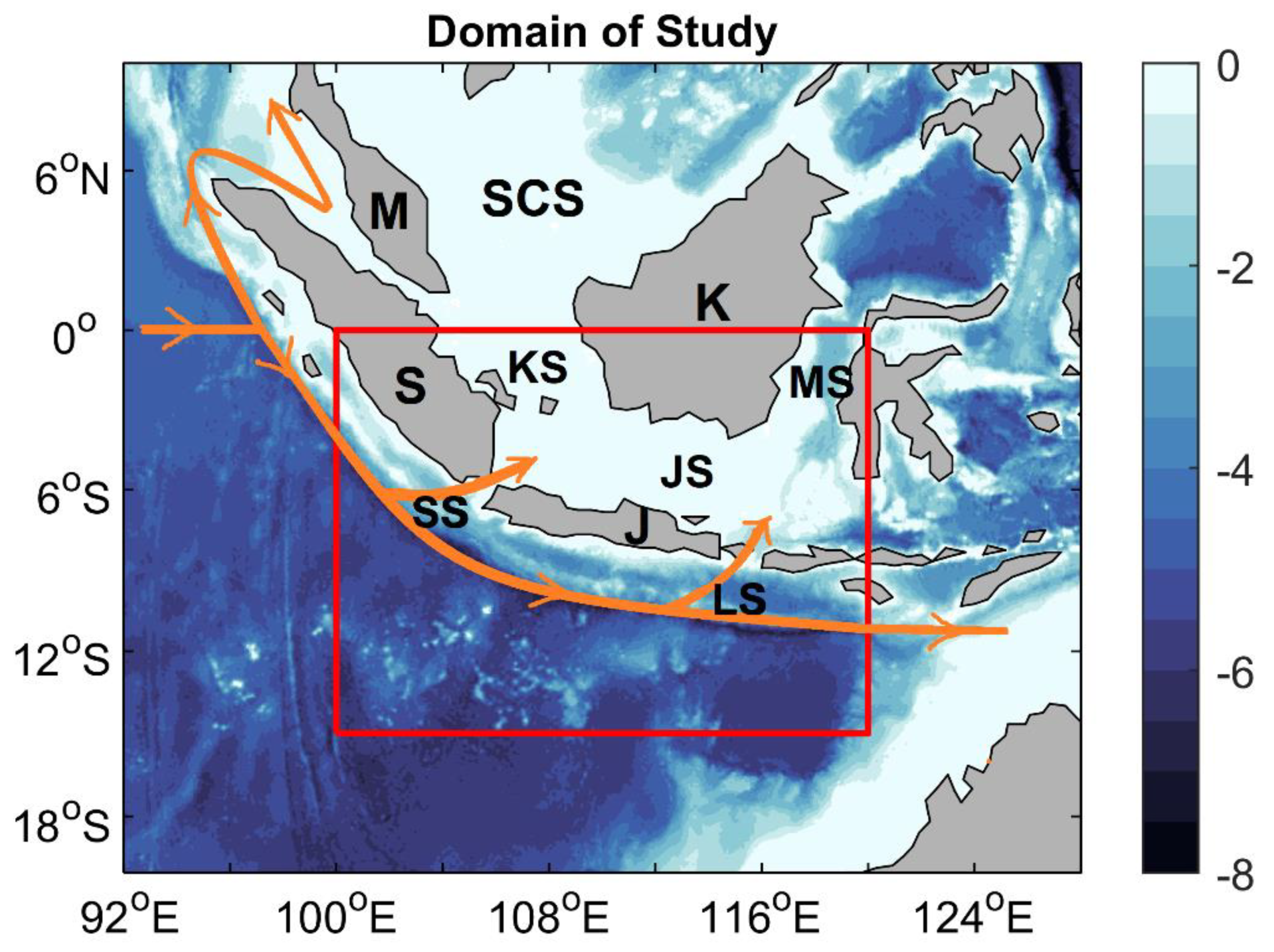
Java Island is located on the southernmost tip of the Maritime continents, where the south Java coast is well known for high primary productivity and plentiful fisheries catch (Figure 1). The domain experiences a seasonal reversal of the monsoonal winds, well associated with precipitation events, i.e., the dry southeast monsoon (SEM) during June–September and the wet northwest monsoon (NWM) during December–March, whereas April–May and October–November represents the monsoon transition periods [13,14]. Several studies have extensively investigated the dynamics of surface chlorophyll-a variability along the south-eastern Indian coast using numerical models, in situ datasets, and satellite datasets on the seasonal time scale [2,15,16,17]. These studies have identified the dynamical factors that can induce the seasonal chlorophyll-a blooms in the domain, such as the Ekman dynamics associated with the seasonally reversing monsoonal winds [18,19] and surface circulation patterns associated with the eastward propagating coastal Kelvin waves [15,16,17,20,21]. Wirasatriya et al. [18] have investigated the contradictory roles of the Ekman mass transport (EMT) and Ekman pumping velocity on the chlorophyll-a variability along the southern coast of Java at the interannual time scale. The role of shoaling thermocline on the upwelling phenomenon off the Sumatra and Java coast associated with the eastward coastal Kelvin waves has been extensively investigated on both the intraseasonal and interannual time scales by Chen et al. [15,16] and Delman et al. [21].
On the other hand, the positive and negative phases of the Indian Ocean Dipole (IOD) and El-Nino Southern Oscillation (ENSO) events strongly modulate the surface chlorophyll-a variability in the tropical Indian Ocean [2,4,20,23,24,25,26,27,28]. Earlier studies have reported the unprecedented surface chlorophyll-a blooms during the 2006 positive IOD event and the 1997/1998 El-Nino event along the south-eastern Indian Ocean [13,20]. Horii et al. [25] have observed a significant decrease in the subsurface temperature within the thermocline, with westward subsurface currents three months before the genesis of the 2006 positive IOD event, as observed from the moored buoys [25]. At the interannual time scale, Rao et al. [29] and Currie et al. [30] have investigated the subsurface thermocline variability and associated chlorophyll-a variability in the tropical Indian Ocean due to the impact of IOD events using the biophysical Ocean General Circulation Models [29,30]. In recent times, Du et al. [31] have identified the downwelling Rossby Waves as the critical parameter for the prolonged IOD event in 2019, triggering the thermocline warming along the southern tropical Indian Ocean and further resulting in the genesis of stronger easterlies along the equator [31]. The interannual variations associated with the Ekman dynamics are substantial in different straits along the coasts and seas within the Maritime Continents [7,18,19,32,33]. However, most of these studies are case studies that have investigated the surface chlorophyll-a variability during positive IOD events or El-Nino events along the south-eastern Indian Ocean.
The present study mainly investigates the spatio–temporal variability of surface chlorophyll-a concentration and associated physical and dynamical factors along the southern Java coast, solely using datasets from multiple satellites and in situ platforms on the seasonal and interannual time scales (Figure 1). Unlike the earlier studies, this study aims to quantify the relative contributions of the physical and dynamical factors, such as SSHA, SST and winds, to the higher chlorophyll-a blooms along the south Java coast using different sets of multiple regression analyses at both time scales. On the interannual time scale, the variations in surface chlorophyll-a concentration have been investigated in terms of composites during the positive IOD events, negative IOD events and normal years. Due to the limited knowledge of surface marine heatwaves (MHW) along the south Java coast, the heatwaves have also been characterized by different MHW metrics. Further, the impact of intense and prolonged MHW events on the surface chlorophyll-a concentration variability has been investigated along the Java Coast in this study.
A brief description of the study area, details of datasets used and methodology adopted are explained in Section 2. The results on seasonal and interannual variabilities of surface chlorophyll-a concentration and other physical parameters defining the ocean surface (SSHA, winds and SST) are discussed in Section 3. Section 4 discusses the possible mechanisms of the surface chlorophyll-a variability along the south Java coast in terms of various dynamical factors at multiple time scales. Section 5 summarizes the conclusions of the present study with some future scopes.
2. Materials and Methods
This section briefly describes the study area in terms of hydrography and seasonal dynamics of the domain in Section 2.1, followed by the details of datasets used in Section 2.2 and detailed methodology in Section 2.3.
2.1. Geographical Setting of Study Area
The Sumatra and Java Islands are essential components of the Maritime Continents along the south-eastern Indian Ocean, where the SEM dominates during the austral winter (i.e., June–September). The southern coast of Java stretches into the south-eastern Indian Ocean with shallow and parallel bathymetric profiles near the coastline, which gradually deepens toward the open sea. However, the bathymetry varies drastically due to the abrupt presence of sea trenches (Figure 1). The straits within these Islands and the southern coasts of Java, Sumatra and the Bali Islands form a significant pathway for the exchange of water masses between the Indian Ocean and the Pacific Ocean.
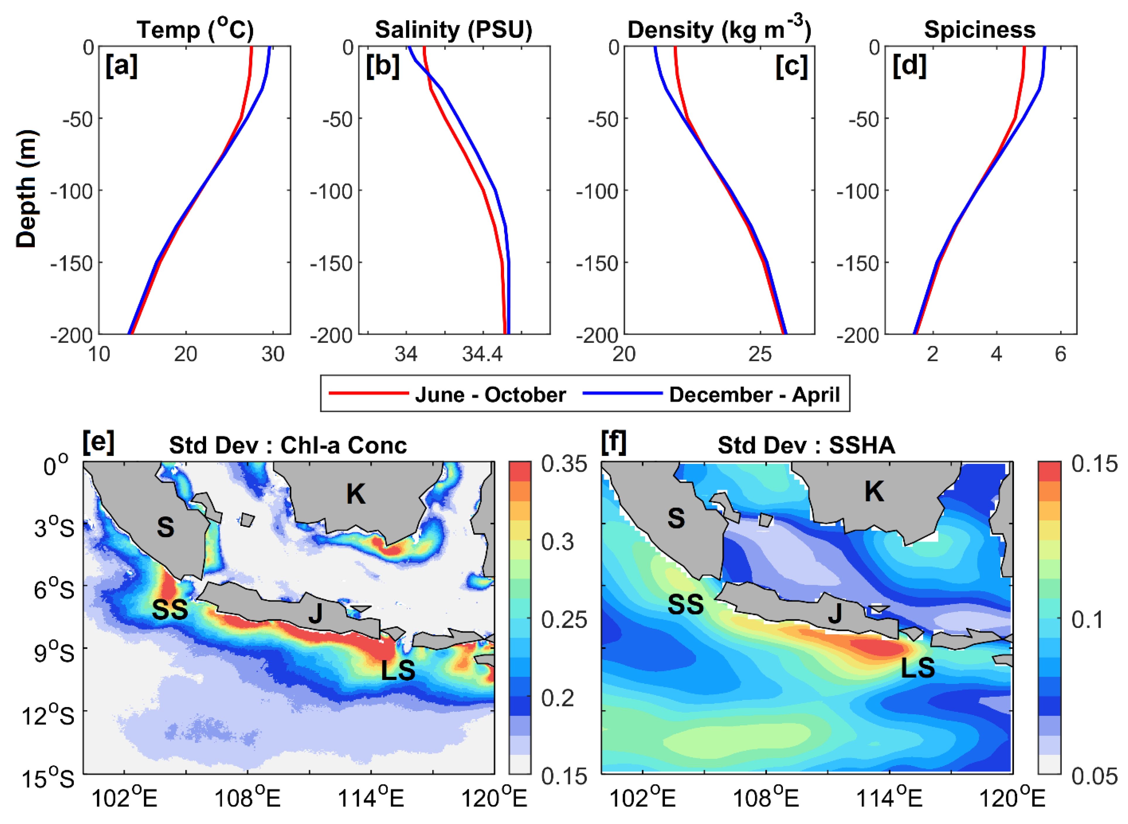
The physical processes along the southern coast of Java and Bali are strongly influenced by the coupled ocean–atmosphere dynamical processes occurring in the Indian Ocean. The climatological temperature, salinity and potential density profiles along the Java coast indicate a significant seasonality within the oceanic mixed layer depth (Figure 2a–d). Lower temperature and higher salinity increase the density of the waters during June–October (SEM), whereas higher temperature and lower salinity make the waters less dense during NWM, December–April (Figure 2a–c). The temperature, salinity and density profiles show prominent signatures of thermocline doming during the southeast monsoon at the seasonal time scale. It can be inferred that the upwelling signatures are significant from the seasonal variations of temperature, salinity and density profiles within the mixed layer during the SEM. Interestingly, a strong seasonality in spiciness (warmer and saltier waters) is also observed along the Java coast. However, the variations in spiciness are strictly restricted to the mixed-layer depth (Figure 2d) and have similar variations to subsurface temperature (Figure 2a). Lower spiciness is observed during the SEM, possibly due to enhanced mixing, whereas spicy waters are apparent in the upper ocean during December–April (NWM). The standard deviation of both surface chlorophyll-a concentration and SSHA indicate higher variations in primary productivity and propagation of the coastal Kelvin waves and south Java coastal currents along the Java coast, which will be discussed in detail in the results section (Figure 2e,f).
2.2. Data
The monthly merged level-4 surface chlorophyll-a concentration data during 2008–2019 from multiple sensors, available at every 4 km (spatial resolution), is extensively utilized in this study to investigate the surface chlorophyll-a variability along the eastern equatorial Indian Ocean (source: https://resources.marine.copernicus.eu/?option=com_csw&view=details&product_id=OCEANCOLOUR_GLO_CHL_L4_REP_OBSERVATIONS_009_082; accessed on 28 November 2021). These surface chlorophyll-a datasets are well-validated against the in-situ observations in the Indian Ocean [17]. The Advanced Scatterometer (ASCAT) observed daily 10 m winds on the ocean surface, available at every 25 km during 2008–2019, and is utilized to investigate the seasonal variability of surface winds [34,35] (source: http://apdrc.soest.hawaii.edu/datadoc/ascat.php; accessed on 28 November 2021). Further, the sea surface height anomaly (SSHA) data during 2008–2019, accessible every month at a spatial resolution of 0.25° × 0.25° from the Archiving, Validation, and Interpretation of Satellite Oceanographic (AVISO) altimetry, is utilized to investigate the sea-level variability along the Java coast, and further diagnose the surface circulation variability in the south-eastern Indian Ocean (source: https://resources.marine.copernicus.eu/product-detail/SEALEVEL_GLO_PHY_L4_MY_008_047/; accessed on 28 November 2021). The daily gridded SST product from the Group for High-Resolution Sea Surface Temperature (GHRSST) data, available every 5 km from 2008–2019, supports and examines the oceanic processes observed along the southern coast of Java and Sumatra (source: https://podaac.jpl.nasa.gov/GHRSST/; accessed on 28 November 2021). Additionally, the water mass characteristics and subsurface variations along the Java coast are investigated utilizing the gridded subsurface salinity and temperature datasets from Argo at the spatial resolution of 1° × 1° every month (source: http://apdrc.soest.hawaii.edu/las/v6/dataset?catitem=201; accessed on 28 November 2021). To investigate the interannual variabilities, the dipole mode index (DMI) is obtained from the Japan Agency for Marine-Earth Science and Technology during 2008–2019 (source: http://www.jamstec.go.jp/frsgc/research/d1/iod/dmi.html; accessed on 28 November 2021). On the other hand, the Nino 3.4 index, extensively utilized to characterize the El-Nino and La-Lina events, is obtained from the Climate Prediction Center (CPC) of the National Oceanic and Atmospheric Administration (NOAA) during the simultaneous time period 2008–2019 (source: http://www.cpc.ncep.noaa.gov/data/indices/sstoi.indices; accessed on 28 November 2021).
2.3. Methodology
Firstly, the seasonal dynamics of the eastern equatorial Indian Ocean have been investigated using climatological datasets, prepared by averaging multiple datasets from various observation platforms during 2008–2019. Secondly, the interannual variability of all the physical parameters has been examined, prepared by removing the climatology from the detrended datasets during 2008–2019. The physical mechanisms responsible for the unprecedented chlorophyll-a blooms during June–October are investigated in terms of various sets of multiple regression analyses on both time scales. The different sets of multiple regression analyses to quantify the relative contributions of the dynamical forcings on seasonal and interannual time scales are discussed in detail in Section 3.1.3 and Section 3.2.3, respectively. Further, the response of chlorophyll-a concentration to the coupled ocean–atmosphere feedback during the positive and negative phases of IOD events is examined through composite analysis. The DMI is extensively utilized to distinguish the positive IOD, negative IOD and normal years during 2008–2019. A year is considered a typical positive (negative) IOD year if the DMI index has values above (below) +0.4 (−0.4) °C consistent with a running standard deviation greater than or equal to 1 (−1) for at least four months [23,36]. On the other hand, the Nino 3.4 index is extensively utilized to characterize the El-Nino and La-Lina events, during the concurrent time period 2008–2019. The years with values beyond +1.5 (−1.5) °C are considered strong El Nino (La Nina) years.
In this study, the surface MHWs have been characterized along the south Java coast using the higher-resolution SSTs during 2008–2019. An event with SST higher than the baseline climatological SST is defined as an MHW event, provided the event is discrete and lasts for a minimum of five or more days with anomalous temperatures warmer than the 90th percentile. A detailed description of the MHW definition can be found in [37]. The interannual variation of these MHWs is analyzed in terms of their cumulative intensity, frequency, area coverage and the number of MHW days. The curious case of strong and prolonged MHW events during 2016 has been characterized, and an effort has been put to relate the surface chlorophyll-a variability and MHWs.
3. Results
This section discusses the seasonal variability of surface chlorophyll-a concentration and other physical parameters in Section 3.1, followed by interannual variations of all the parameters and the impacts of ENSO and IOD events on the surface chlorophyll-a variability in Section 3.2. The possible mechanisms and associated dynamical factors modulating the surface chlorophyll-a variability are discussed in terms of various sets of multiple regression analyses of the parameters in Section 3.2. The interannual variability of surface MHWs along the southern Java coast is discussed in Section 3.3 in terms of different MHW metrics. The impact of the strongest and most prolonged MHW event on the chlorophyll-a variability during 2016 for possible ecological impacts is discussed in the same section.
3.1. Seasonal Variability
3.1.1. Variability of Chlorophyll-a Concentration
The standard deviation map of surface chlorophyll-a concentration shows higher values (>0.32 mg m−3) along the southern Java coast, indicating higher chlorophyll-a variability in the domain (Figure 2e). Also, higher chlorophyll-a variability can be observed in the nearby regions of Sunda Strait and Lombok Strait, which could be due to the nutrient-rich water supplies from the Indonesian throughflow [38]. Note that the higher values of the standard deviation of chlorophyll-a concentration are persistent throughout the year along the northern Java Sea. In contrast, a strong seasonality is significantly observed along the southern Java coast with chlorophyll-a blooms during the SEM (June–October) compared to the lower chlorophyll-a concentration values during December–April in the northwest monsoon (Figure 3a,b).
The probable dynamic and physical factors influencing this strong seasonality of surface chlorophyll-a concentration could be the seasonal variations in coastal upwelling (through Ekman Mass Transport, EMT), SST, the role of wind stress curl and SSHA (particularly to understand the influence of coastal currents and Kelvin Waves).
3.1.2. Variability of SST, Winds, and SSHA
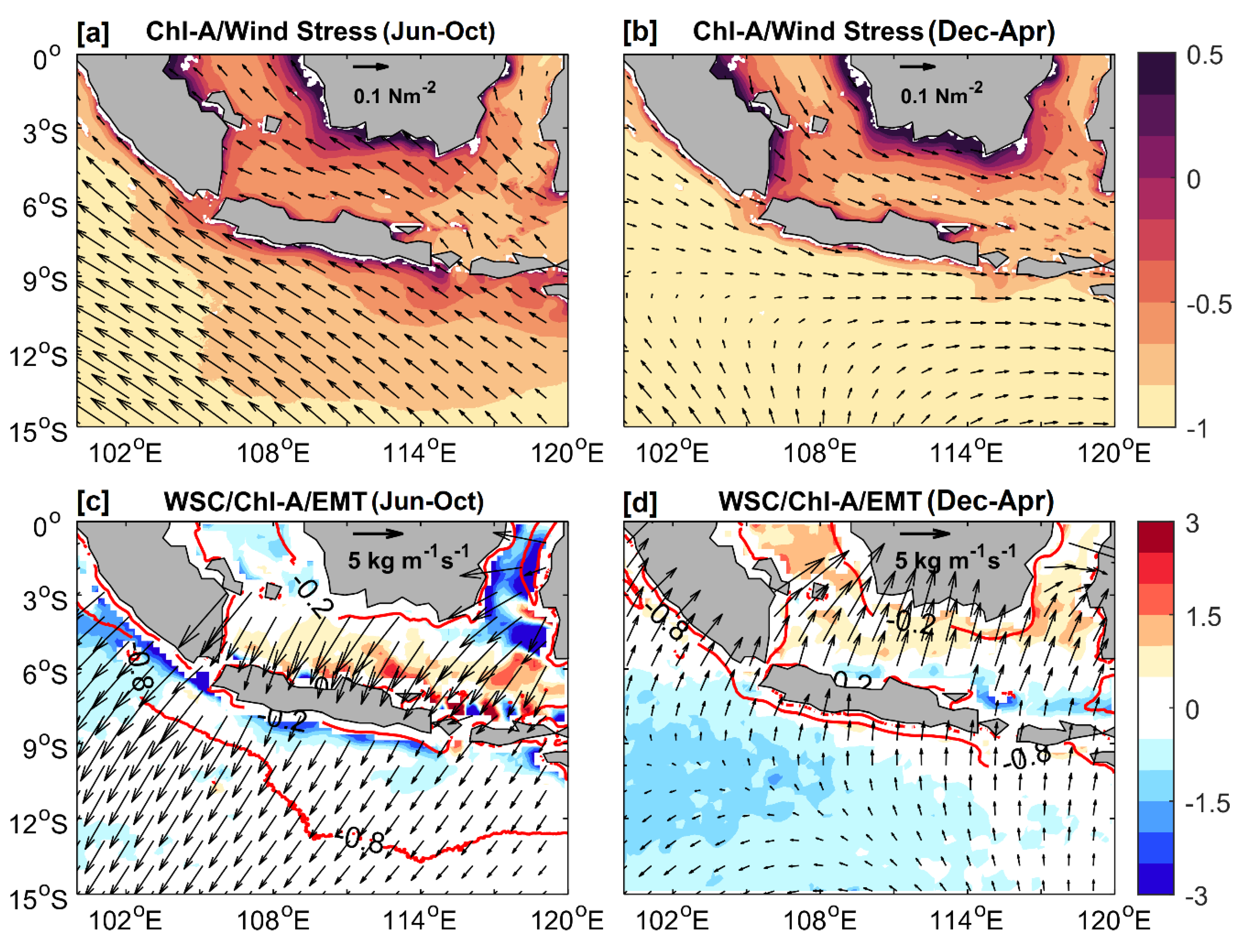
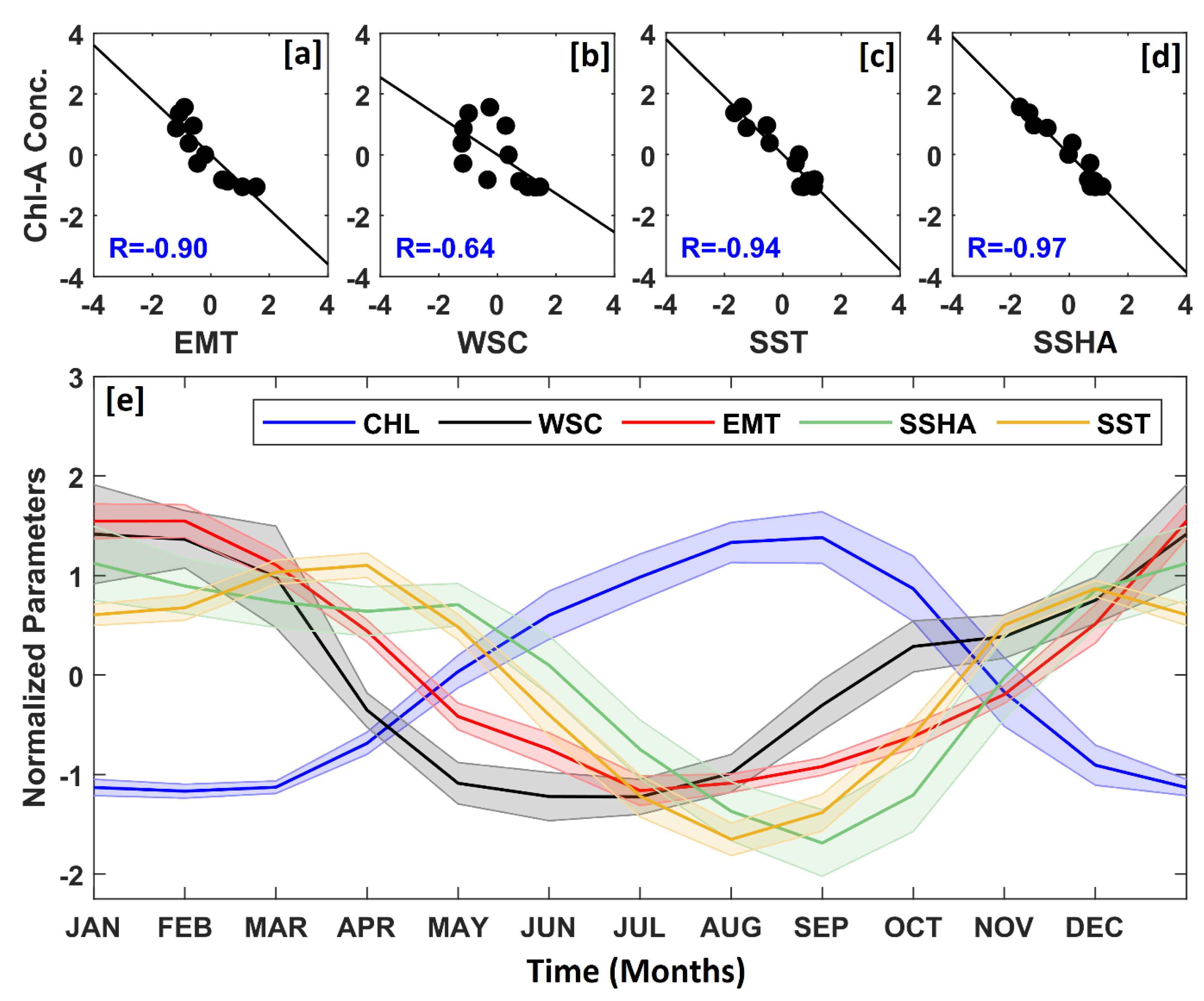
The seasonal reversal of monsoonal winds is significantly observed over the domain, i.e., the north-westerlies during December–February (wind speed of ~5.62 m s−1) and the strong south-easterlies during June–October (wind speed of ~7.82 m s−1). Figure 3a,b show a strong seasonality of surface wind stress along the southern Java coast with higher stress during the SEM (~0.14 N m−2) than during the NWM (<0.05 N m−2). It is interesting to note that the maximum values of negative wind stress curl (nearly −2.1 × 10⁻⁷ N m−3) are observed during June–October along the southern Java coast, which leads to enhanced upwelling with the onset of SEM and is well supported by the higher chlorophyll-a blooms in the domain (Figure 3c). However, the near-positive values of wind stress curl during the northwest monsoon observed along the Java coast indicate reduced upwelling/downwelling features, along with the lowest chlorophyll-a concentration values during December–April (Figure 3d). Strong seasonality of EMT is also observed along the Java coast to the left of the wind direction. The south-westward offshore transport is quite prominent during June–October concurrent to the vast spatial extent of higher chlorophyll-a waters off the southern Java coast (red contour in Figure 3c). Moreover, the coastal upwelling phenomenon has significantly reduced in the domain with inshore transport in the north-eastward direction during the NWM (Figure 3d). The EMT and wind stress curl have reasonable correlations of −0.90 and −0.64 with chlorophyll-a concentration, respectively. However, the correlation coefficient increases (−0.90) for wind stress curl when correlated with chlorophyll-a concentration, provided the wind stress curl leads by two months.
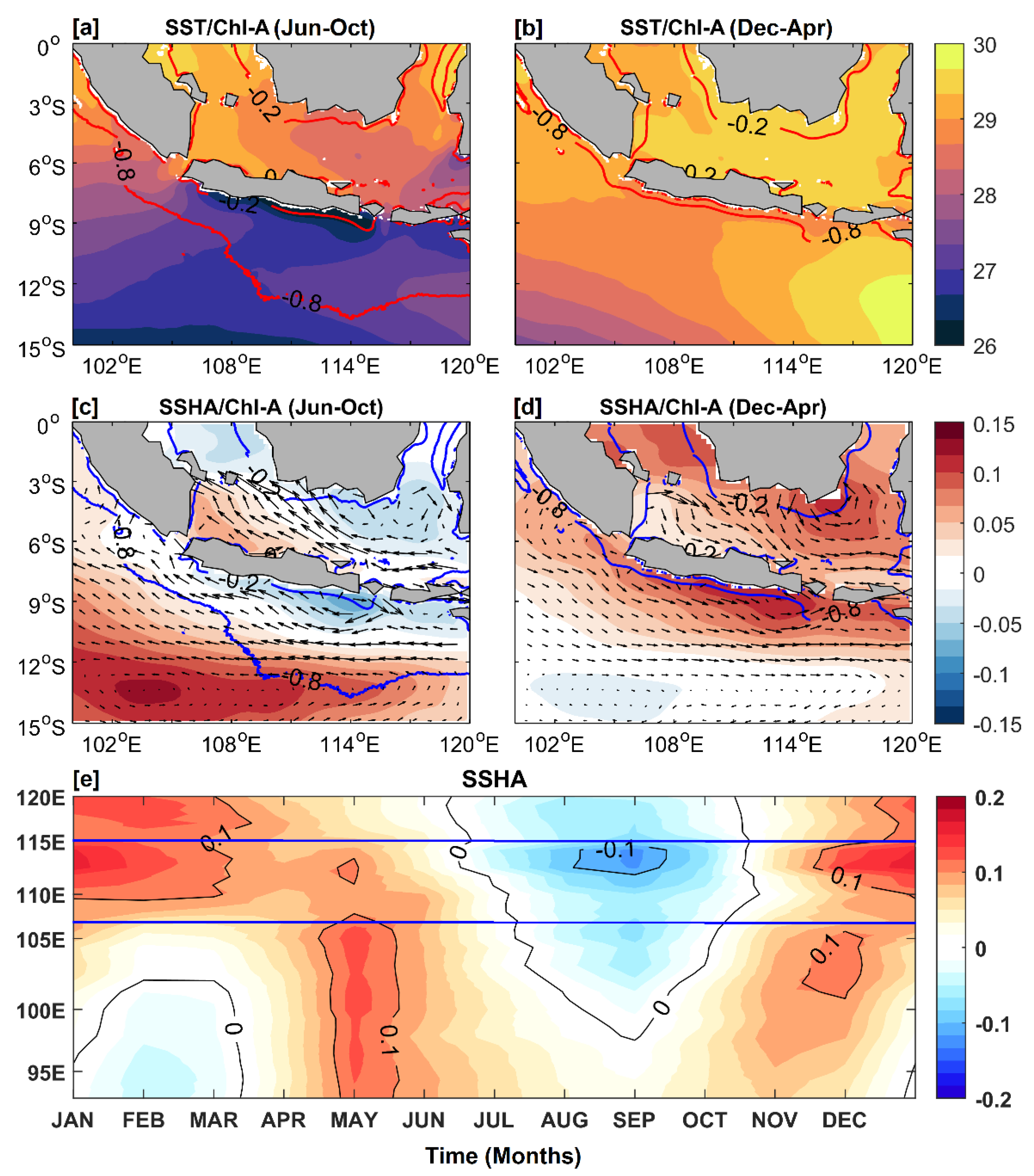
The SST plays an essential role in representing the upper ocean physical processes, specifically, the upwelling processes associated with eddies, fronts and filaments and surface circulation features. Warmer SSTs (~29.5 °C) are apparent during December–April (NWM) off the southern coast of Java, whereas comparatively colder SSTs (~26.75 °C) are observed during the SEM (Figure 4a,b). Also, the seasonal variations of water mass properties show signatures of vertical entrainment of dense waters (with higher salinity and lower temperature) from the subsurface during SEM (Figure 2a–d). These upwelling signatures are evident from the significant reduction in SST by ~2.75 °C during the SEM. The region-averaged SST has a significantly higher correlation of −0.94 (at 95% significance level) with the same for chlorophyll-a concentration within the domain, i.e., lower SSTs are linked to higher chlorophyll-a concentration and vice-versa (Figure 5c).
The seasonally reversing nature of boundary currents (commonly known as the south Java coastal current) is significantly observed along the southern coast of Java, i.e., the surface currents flow north-westward during the SEM period (June–October) and south-eastward during the NEM in December–April [3,39,40]. It is interesting to note that the propagation of the upwelling and downwelling phases of coastal Kelvin waves is limited to 105°E until the Sunda Strait (Figure 4e). However, signatures of the seasonally reversing south Java coastal current are prominent along the southern Java coast (Figure 4c,d). The seasonal sea-level variations along the south Java coast are investigated using the seasonally averaged SSHA during 2008–2019 (cyan contours in Figure 4c,d). The seasonal variations of SSHA show prominent signatures of a matured coastal ocean cyclonic eddy during the SEM (June–October) and anticyclonic coastal eddy during the NWM (December–April), well-supported by the variations in chlorophyll-a concentration and SST during the different seasons (Figure 4c,d). The mesoscale cyclonic eddies are responsible for the eddy-induced upwelling associated with negative sea surface height anomalies. Further, the highest correlation (−0.97 with p-value < 0.001) is found between the region-averaged chlorophyll-a concentration and SSHA in the domain, i.e., the chlorophyll-a blooms are directly linked to negative sea surface height anomalies during the SEM and vice-versa (Figure 5d). This is interesting to note that the chlorophyll-a concentration attains the highest correlations with SST and SSHA without any lags.
3.1.3. Relative Roles of Dynamical Factors controlling the Surface Chlorophyll-a Concentration Variability (Quantifying Seasonal Variability)
The above results on the seasonal chlorophyll-a variability indicate significant inter-relationship with various dynamical factors, like the sea level anomalies, SST, EMT and wind stress curl, well-supported by the direct correlation coefficients. The monthly climatological data is prepared by averaging fourteen years (2008–2019) of region-averaged monthly data for each of these variables. The standard errors are also calculated (shaded background in Figure 5e) to investigate the seasonality and standard deviations during a particular time. Figure 5e shows the seasonality of all these physical and dynamical factors that can significantly modulate the variations in chlorophyll-a concentration along the south Java coast. In addition, three separate sets of multiple regressions have been performed to evaluate the relative contributions of these dynamical factors impacting the chlorophyll-a concentration seasonal variations.
One of the most important physical characteristics for understanding upwelling is SST. The warmer waters on the ocean surface reduce the vertical mixing in the upper ocean, i.e., less mixing between the surface and deeper waters, which actually reduces the presence of nutrient-rich waters on the surface. With the scarcity of nutrient-rich waters at the surface, where phytoplankton grow, the surface chlorophyll-a concentration also declines. A significantly strong correlation (−0.94 with p-value <0.001) is observed between SST and chlorophyll-a concentration along the coastal regions of south Java (Figure 5c and top panel of Figure 4). Moreover, the surface winds also play an essential role in triggering the upwelling phenomenon along the coastline in terms of wind-driven mixing (i.e., the entrainment of cold, saline, and dense waters) and coastal upwelling (i.e., favorable EMT). This leads to the vertical transport of nutrients, resulting in surface chlorophyll-a blooms. Note that the signatures of coastal upwelling are significant and prominent in the domain, which is well supported by a higher correlation of chlorophyll-a concentration with EMT. Also, thermocline doming is evident from the temperature and salinity profiles during the concurrent time period (June to October). Higher correlations with EMT indicate the dominance of the coastal upwelling phenomenon over the wind stress curl-induced upwelling. Moreover, the south-easterlies, from June to October, induce an upwelling favorable wind stress curl along the south Java coast, lowering the sea levels (negative SSHA) and reducing the SST, followed by the entrainment of cold and saline subsurface waters to the surface, resulting in intense chlorophyll-a blooms (Figure 4). The upwelling favorable south-easterly winds are ideal for propelling a cyclonic eddy-like structure associated with the north-westward south Java coastal current (SJCC) during June–October, resulting in chlorophyll-a blooms at the surface, apparent from the highest correlation coefficient (−0.97 with p-value < 0.001) between SSHA and chlorophyll-a concentration (Figure 5d). Higher correlations at 95% significance levels between chlorophyll-a concentration and other physical parameters (SSHA, EMT, SST and wind stress curl) evidently indicate that all the physical parameters have concomitantly influenced the chlorophyll-a levels in the domain with no lags.
The inter-relationship between the different dynamic parameters makes it tough to identify the dominant factor that significantly contributes to the upwelling phenomenon in the domain. So, multiple regression analysis has been performed for the following three model combinations at the seasonal time scale. In model A, the chlorophyll-a concentration is represented as a combination of all other physical parameters. Similarly, chlorophyll-a concentration is defined as a combination of SSHA, SST and EMT in model B, whereas model C represents the chlorophyll-a concentration as a combination of wind stress curl, SST and EMT (Table 1).
In the first and second models (models A and B), it is interesting to note that the SSHA and associated surface circulation variability (i.e., the south Java coastal currents) are the dominant forcings responsible for the higher chlorophyll-a concentration along the southern Java coast, followed by the coastal upwelling due to EMT and SST (Table 1). The wind stress curl, on the other hand, makes a negligible contribution to the increased variability of chlorophyll-a concentration in the domain. Two separate multiple regressions have been preferred to further differentiate between the contributions of SST and EMT in the domain. When the dependence of chlorophyll-a concentration on all physical parameters except SSHA is explored in the third model (Model C), it is noteworthy to notice that the coastal upwelling phenomenon produced by EMT plays a considerable role over SST in the domain. (Table 1).
3.2. Interannual Variability
3.2.1. Variability of Chlorophyll-a Concentration
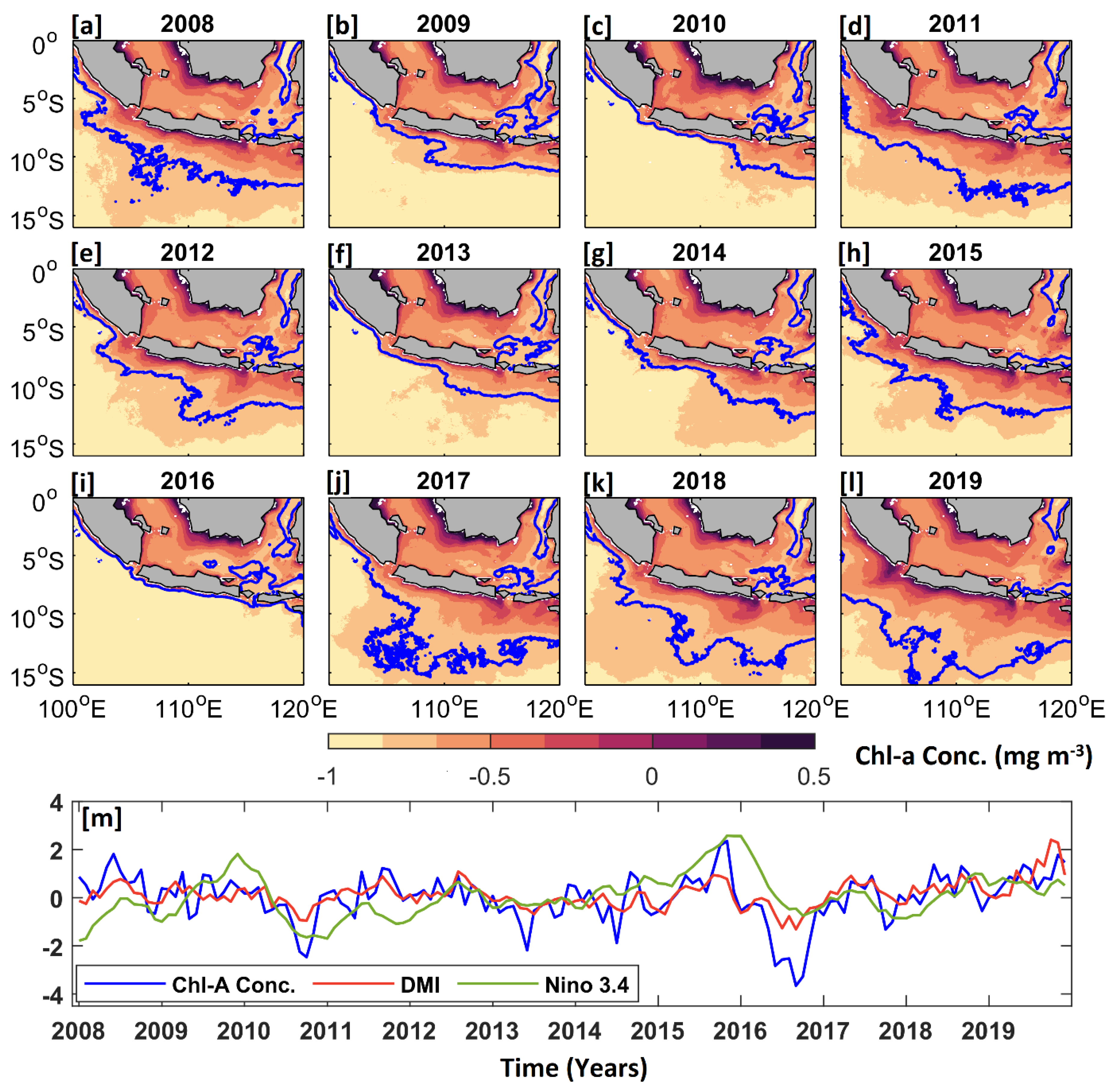
In the previous sections, significant signatures of chlorophyll-a blooms are observed during June–October from the seasonal chlorophyll-a concentration data. Strong effects of SSHA, EMT and SST on chlorophyll-a concentration are also observed on the seasonal time scale from the various sets of multiple regression analysis. The south-eastern Indian Ocean is known to be strongly influenced by large-scale climate phenomena, such as ENSO and IOD. Thus, investigating the interannual variability of the surface chlorophyll-a concentration and quantification of the dynamical factors contributing to the interannual chlorophyll-a variations during the upwelling season is essential during the period 2008–2019. This section is particularly focused on investigating the interannual variations in chlorophyll-a concentration along the south Java coast. Figure 6 shows the spatial distribution of surface chlorophyll-a concentration maps averaged during the upwelling season (i.e., June to October) along the south Java coast during 2008–2019.
Interannual variations are significantly observed in spatial distribution chlorophyll-a concentration during 2008–2019. Significantly higher values and larger spatial extent of chlorophyll-a concentration are observed in 2008, 2012, 2015, 2017, 2018 and 2019, whereas the least values of chlorophyll-a concentration with negligible spatial extent are observed in 2010 and 2016 (Figure 6a–l). The correlation between region-averaged, climatology-removed and detrended surface chlorophyll-a data with DMI is higher (0.68) than that observed with Nino 3.4 index (0.28), indicating a higher impact of IOD events on the primary productivity in the domain (Figure 6m).
Following the higher impact of IOD events in the domain, the next section focuses on the composite analysis of all the physical parameters based on the identified positive and negative phases of the IOD events during the analysis period.
3.2.2. Impact of Indian Ocean Dipole (IOD) Events
The upper ocean dynamics along the south-eastern Indian Ocean play a significant role in the evolution of the IOD events. Figure 6m shows the temporal variability of DMI during 2008–2019, from which the positive IOD (2008, 2012, 2015, 2017, 2018 and 2019), negative IOD (2010 and 2016) and the normal years (2009, 2011, 2013 and 2014) have been distinguished. With respect to the normal years, the linked ocean–atmosphere phenomenon related to the impact of positive and negative IOD events on surface chlorophyll-a variability has been thoroughly examined utilizing composite analysis (Figure 7).
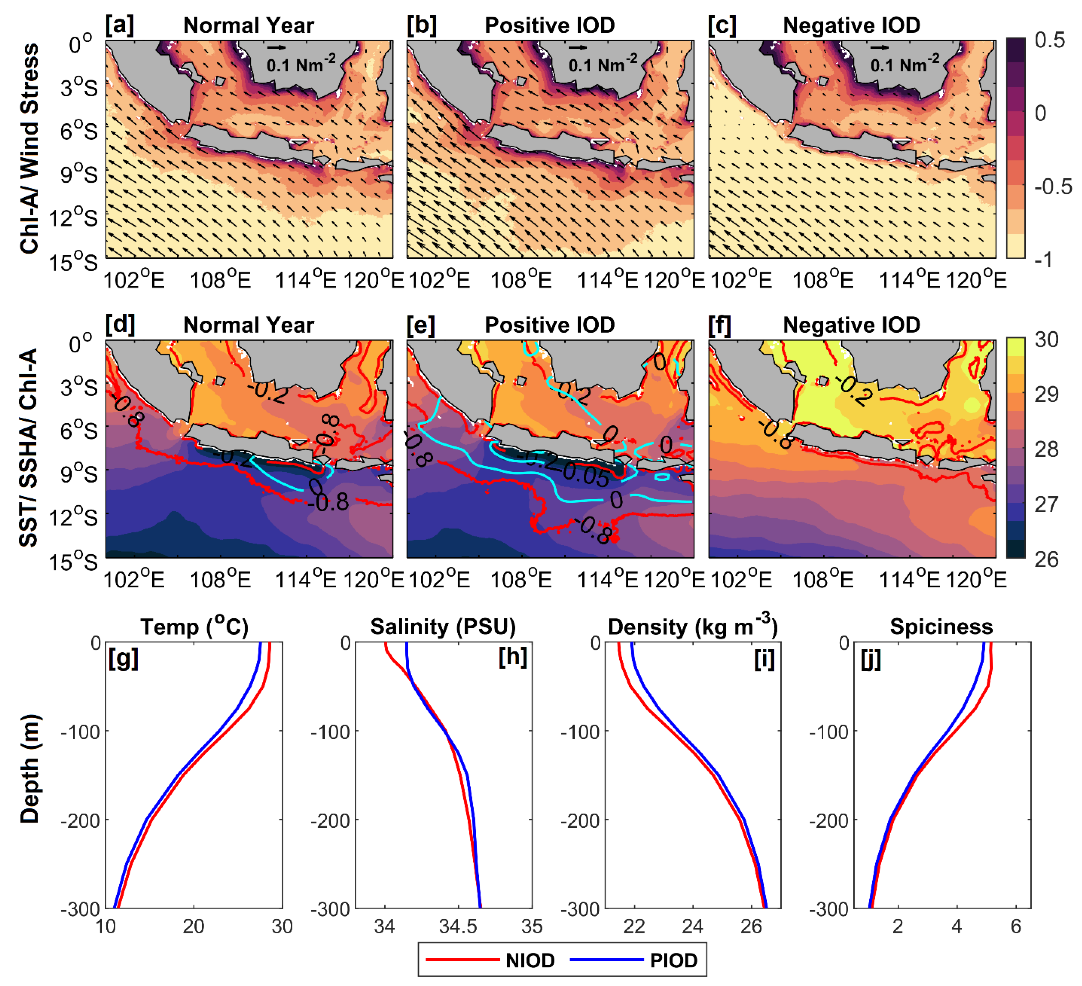
During the normal years (i.e., neither an IOD nor an ENSO event), comparatively higher wind stress during the SEM (during June–October) associated with the south-easterlies is observed to induce strong offshore Ekman mass transport along the southern coast of Java (Figure 7a). At the same time, cold SSTs and reduced sea levels are observed, well-supported by the entrainment of cold, saline and low spice dense waters due to the well-developed cyclonic eddy along the south Java coast (Figure 7d). As a result, a moderate increase in surface chlorophyll-a values is observed along the southern coast of Java during the normal years in the SEM from June–October (Figure 7a,d). On the other hand, a substantial strengthening of the wind stress is observed during the SEM (during June–October), with the intensification of south-easterlies along the south coast of Java during the positive IOD years. Linked to these intensified south-easterly winds, the negative sea level anomalies and coldest SSTs are observed off the south Java coast accompanied by intense chlorophyll-a blooms (Figure 7b,e). The most robust offshore Ekman mass transport concurrent to intensified coastal upwelling is observed during pIOD events, which results in the advection of surface chlorophyll-a concentration off Java (Figure 7b). The entrainment of the colder and saltier waters from the subsurface with higher density and lower spiciness is significantly observed within the mixed layer depth (Figure 7g–j). Consequently, colder SST (<25.4 °C) along with an intensified cyclonic eddy (with SSHA less than −10 cm) is observed off the south Java coast (Figure 7e). As a result, maximum chlorophyll-a concentration was observed along the south Java coast as well as in the offshore regions during the pIOD events (Figure 7b). In contrast, comparatively weak south-easterlies are observed during the negative IOD years off the Java coast, leading to negligible Ekman mass transport and weak coastal upwelling (Figure 6c). The weak alongshore wind stress leads to increased positive SSHAs (i.e., absence of the cyclonic eddy) and comparatively high SSTs (>28.8 °C) along the south Java coast (Figure 6f). As a result, the chlorophyll-a concentration has significantly reduced in the domain, well-supported by comparatively less dense waters with higher temperature, lower salinity and higher spiciness, all restricted within the mixed layer depth (Figure 6g–j).
Thus, it can be concluded that the least surface chlorophyll-a concentration is observed during the negative IOD events as compared to the highest observed during the positive IOD years along the south Java coast, which can be attributed to the lower surface wind stress and mild signatures of mesoscale cyclonic eddy-induced weakened upwelling, and well-supported by warm and low saline waters (higher SSTs) on the surface during the negative IOD years.
3.2.3. Relative Roles of Dynamical Factors controlling the Surface Chlorophyll-a Concentration Variability (Quantifying Interannual Variability)
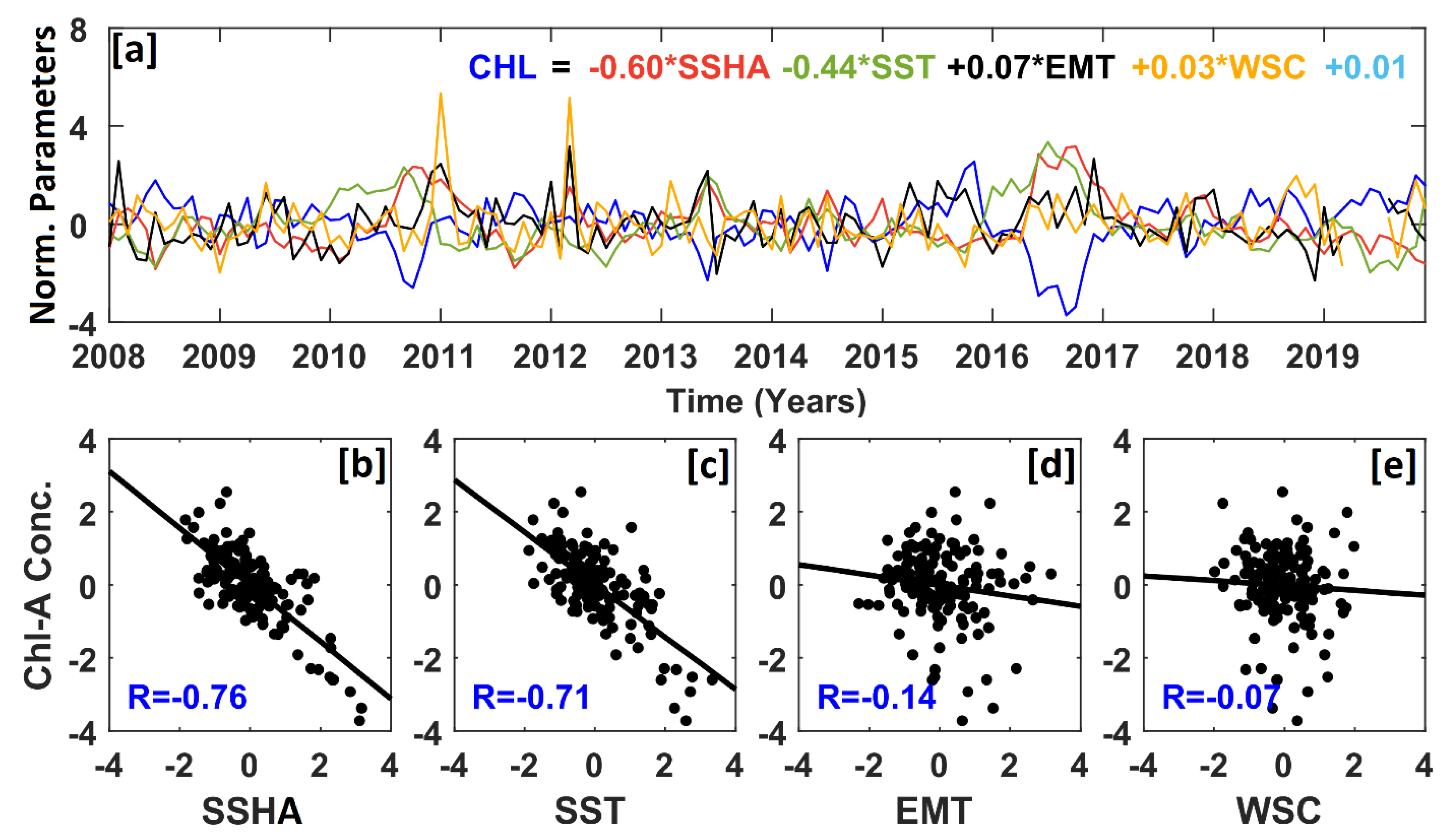
Looking at the interannual variability, the lower values of chlorophyll-a concentration are observed during 2010 and 2016, along with higher SSTs and SSHAs along the south Java coast. Thus, a similar multiple regression analysis has been performed on the interannual time scale to determine the most significant contributing factor to the chlorophyll-a variability in the domain. Here, chlorophyll-a concentration is represented as a combination of other physical factors such as SSHA, SST, EMT and WSC. The multiple regression analysis of all the physical parameters evidently indicates the highest dependence of chlorophyll-a concentration on the sea level anomalies (−0.60), followed by its dependence on SST (−0.44), EMT (+0.07) and WSC (+0.03) (Figure 8a). However, beta coefficients corresponding to Ekman mass transport and WSC are not statistically significant. On the other hand, one-to-one correlations of chlorophyll-a concentration with other parameters indicate a higher correlation with SSHA (−0.76), followed by SST (−0.71), EMT (−0.14) and WSC (−0.07) (Figure 8b–e). It is interesting to note that in either of the cases (multiple regression analysis and one-to-one correlation analysis), the SSHA-induced mesoscale cyclonic eddies and associated surface circulation pattern are the most prominent contributing factors to the higher values of surface chlorophyll-a concentration during the SEM (June–October) along the south Java coast, well supported in the cold waters with lower SST.
3.3. Curious Case of Marine Heatwave Event during 2016
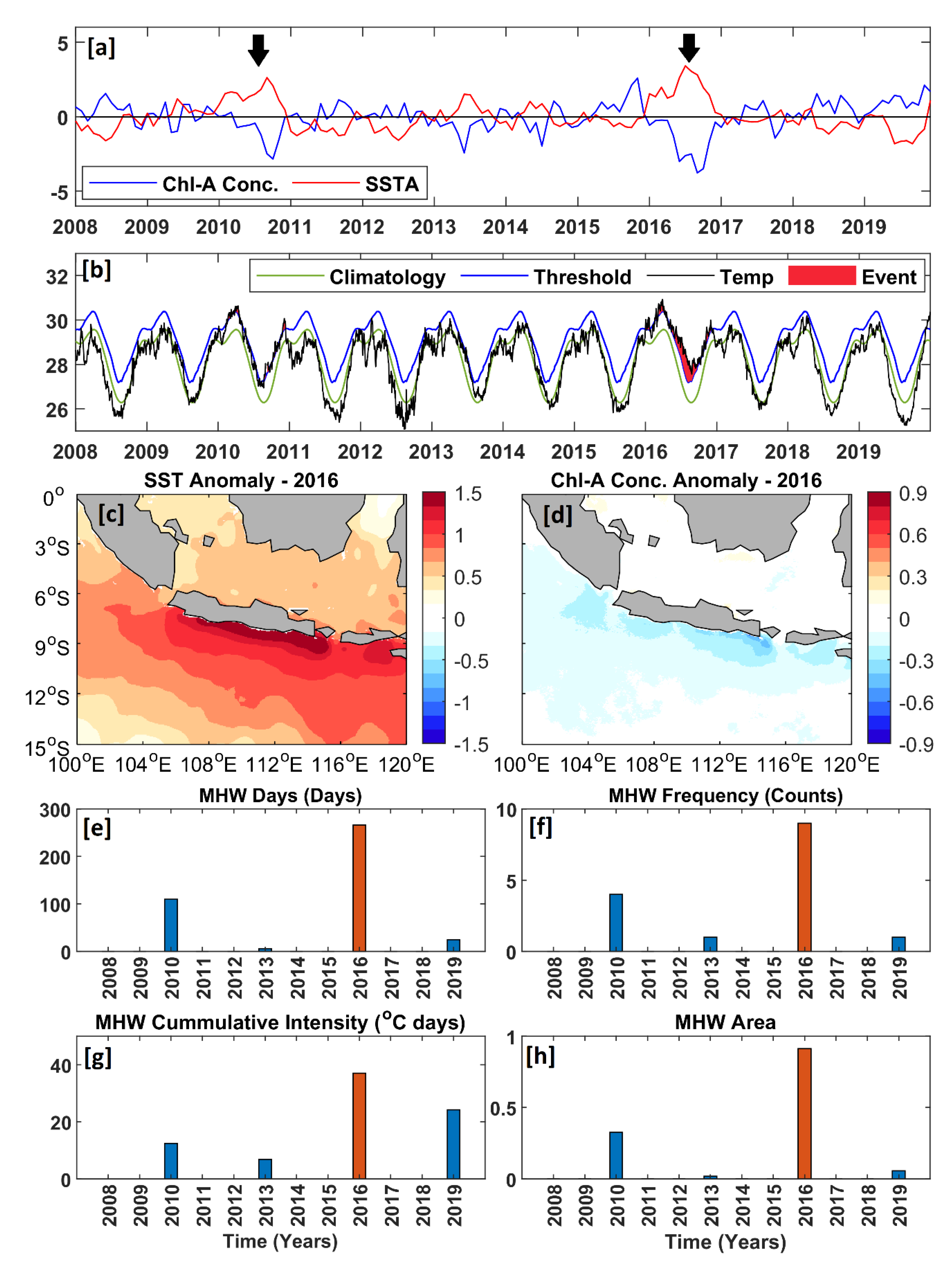
In recent decades, the MHWs are drastically influencing the marine ecosystem in terms of coral bleaching, increasing the mortality rate of fisheries and marine invertebrates, including a huge reduction in the surface chlorophyll-a concentration throughout the world’s coasts [41,42]. This section focuses on the characterization of the surface MHWs along the southern coast of Java during 2008–2019 (Figure 9). Figure 9a represents the temporal evolution of spatially averaged, climatology removed and normalized surface chlorophyll-a concentrations and SSTs during 2008–2019. Significantly higher SST anomalies and lowest chlorophyll-a concentration anomalies are observed along the southern coast of Java during 2010 and 2016, which are the substantially strong negative IOD years (indicated by black arrows in Figure 9a). The unprecedented higher SSTs during 2016 indicated the presence of an MHW event during 2016 (Figure 9b). The highest SST anomaly (nearly 3 °C warmer) and lowest chlorophyll-a concentration anomaly are observed during the year 2016. Similar signatures can also be seen from the spatial distributions of climatology-removed SST anomalies and chlorophyll-a concentrations in 2016 (Figure 9c,d). According to the MHW definition [37], applied to daily GHRSST data during 2008–2019, the southern coast of Java experienced prolonged and continuously intense MHWs during 2016 (red shaded region in Figure 9b). The MHW event has a maximum intensity of 1.28 °C, a mean intensity of 1 °C, cumulative intensity of 37.06 °C days and persisted in the domain for a duration of 270 days with a maximum area coverage during 2016 (Figure 9e–h). The MHW metrics characterize this event as the strongest MHW event to date. In summary, this event is both the longest and the most intense MHW on record along the south coast of Java.
4. Discussion
The southern coast of the Java Islands is well-known for seasonal upwelling, making it rich in fisheries catch during June–October (i.e., SEM). Higher values of surface chlorophyll-a concentration are observed during the SEM, than during December–April (i.e., NWM). Unlike earlier studies, this study focuses on quantifying the relative contributions from the different dynamical factors to the seasonal chlorophyll-a variability using multiple regression analyses.
The north-westward wind stress is significantly observed during May–June, which induces offshore EMT leading to coastal upwelling along the southern Java coast. Simultaneously, the strengthening of north-westward SJCC associated with a matured mesoscale cyclonic eddy is also observed in the domain leading to thermocline doming, well-supported by the presence of dense waters with reduced SSTs on the ocean surface, indicating strengthened upwelling along the south Java coast. This upwelling phenomenon leads to higher chlorophyll-a blooms during the SEM. Different combinations of multiple regression analyses on the seasonal time scale also indicate the dominant role of eddies and EMT in the higher chlorophyll-a blooms during June–October along the south Java coast. The vast spatial extent of chlorophyll-a concentration off Java can be attributed to the eddy-induced upwelling. Note that the influxes from Indonesian throughflow during October may also bring nutrient-rich waters to the Java coast through the Sunda Strait and Lombok strait, which may also increase the chlorophyll-a concentration in the domain [17,38]. The surface chlorophyll-a concentration decreases during November, with the onset of the NWM associated with strong north-westerlies. With the increase in south-eastward wind stress, the EMT reduces, and negligible coastal upwelling is observed from December–April. Simultaneous variations are observed in the upper ocean with positive anomalies of SSHA and warm SSTs along the south coast of Java, resulting in a significant decline in the chlorophyll-a concentration.
On the interannual time scale, the presence of the mesoscale cyclonic eddy associated with SJCC along the south Java coast plays a prominent role in the higher chlorophyll-a blooms every year, followed by the relative roles of SSTs and EMT. The chlorophyll-a concentration peaks during the strong pIOD years, which is attributed to the presence of the cold and dense waters on the ocean surface due to intense thermocline doming, well forced by strengthened south-easterlies along the south Java coast. On the other hand, the chlorophyll-a concentration substantially reduced during the strong nIOD years, which is well supported by the deepening of the thermocline, positive SSHAs and comparatively warm SST anomalies on the ocean surface, all indicating reduced upwelling. The mesoscale eddies associated with south Java currents played a prominent role in modulating the surface chlorophyll-a concentration along the south Java coast on both the seasonal and interannual time scales. Another interesting phenomenon is the least surface chlorophyll-a concentrations between 2010 and 2016, which is attributed to the highest SST anomalies associated with the intense and prolonged surface MHWs in the domain.
Thus, it can be concluded that mesoscale cyclonic eddies associated with the strong south Java currents lead to intense surface chlorophyll-a blooms and upwelling phenomenon during the SEM through strong Ekman mass transport on the seasonal time scale. On the other hand, the warmer SSTs play a significant role over the EMT on the interannual time scale, provided the mesoscale cyclonic eddies and associated coastal currents have a dominant role in the domain. Moreover, the subsurface MHWs play a significant role in the drastic decrease in the chlorophyll-a concentrations during the negative IOD years, thereby devastating the marine habitats, ecosystems and fisheries.
5. Conclusions
This study investigates the dynamic factors and physical processes responsible for higher chlorophyll-a concentration during the southeast monsoon (June–October) along the south Java coast using the remotely sensed satellite datasets from 2008–2019 on the seasonal and interannual time scales. The interannual chlorophyll-a variabilities associated with the IOD events during the same period are also investigated. Moreover, the impact of the surface MHWs on the surface chlorophyll-a variability is also investigated along the southern Java coast. The significant results are as follows:
- A seasonality of chlorophyll-a concentration is observed along the south Java coast, with the highest amplitudes (nearly threefold) during the SEM (June–October) and lowest during the NWM (December–March). Analogous seasonal variations are also observed from SSHA, Ekman mass transport, SST and wind stress curl.
- The temperature and salinity profiles also show a strong seasonality with signatures of upwelling during the SEM, well-supported by the entrainment of cold and saline waters with higher density and lower spiciness. In contrast, downwelling signatures with low salinity and high temperature are persistent during the NWM.
- The strong south-easterlies associated with high wind stress drive the north-westward south Java coastal current with a mature mesoscale cyclonic eddy during the SEM. This surface circulation variability and strong offshore Ekman mass transport result in intense coastal upwelling in the domain. During SEM, this upwelling phenomenon is well-supported by colder SSTs and thermocline doming (entrainment of cold and saline waters).
- Multiple regression analysis and the one-to-one direct correlation analysis on the seasonal time scale suggest a dominant role of coastal currents and mesoscale cyclonic eddies in the chlorophyll-a variability, followed by roles of EMT and SST. The wind stress curl has the lowest contribution to the chlorophyll-a variability with minimum correlations.
- On the interannual time scale, strong chlorophyll-a blooms and their large spatial extents are significantly observed during the positive IOD years, which is attributed to the strong signatures of mesoscale cyclonic eddies and strong thermocline doming, well-supported by cold SSTs. In contrast, the minimum upwelling associated with the lowest chlorophyll-a concentration is observed off Java during the negative IOD years, which is attributed to the weakened cyclonic eddies and warm SSTs.
- Least surface chlorophyll-a values are observed during 2010 and 2016, well-associated with higher SST anomalies (nearly 3 °C) and thermocline deepening along the southern Java coast, which can be attributed to the intense, prolonged exposure and continuous surface MHWs during these negative IOD years.
To conclude, this study represents the seasonal and interannual variability of the remotely sensed physical parameters (temperature, salinity, chlorophyll-a concentration, SST, winds and SSHA) from monthly datasets from satellites and Argo, with possible impacts of the surface MHWs of surface chlorophyll-a variability along the south-eastern Indian Ocean. Like the Malacca Strait, the intraseasonal oscillations associated with the Madden–Julian Oscillations may also play an essential role in the surface chlorophyll-a variability along the south Java coast, which needs to be investigated [7,17]. On the other hand, intense and prolonged MHWs are also observed in the domain, which is significantly reducing the biological productivity that feeds the marine ecosystems and fisheries. Owing to the lack of subsurface datasets and studies characterizing the subsurface MHWs along the Java coast, setting up a biophysical model will provide a three-dimensional perspective of the subsurface MHWs and their possible impacts on biological productivity.
Author Contributions
Conceptualization S.M..; validation, S.M.; formal analysis, S.M..; investigation, S.M.; resources, S.M. and B.R.; data curation, S.M..; writing—original draft preparation, S.M.; writing—review and editing, S.M., B.R. and R.D.S..; supervision, S.M.; funding acquisition, R.D.S., S.M. and B.R. All authors have read and agreed to the published version of the manuscript.
Funding
This research was funded by NASA grant number 80NSSC18K0777, and the APC was funded by 80NSSC18K0777.
Data Availability Statement
The surface chlorophyll-a concentration data is available at https://resources.marine.copernicus.eu/?option=com_csw&view=details&product_id=OCEANCOLOUR_GLO_CHL_L4_REP_OBSERVATIONS_009_082 (accessed on 28 November 2021). The GHRSST sea surface temperature data are available at https://podaac.jpl.nasa.gov/GHRSST (accessed on 28 November 2021). The sea surface winds from Advanced Scatterometer (ASCAT) are available at http://apdrc.soest.hawaii.edu/datadoc/ascat.php (accessed on 28 November 2021). The sea surface height anomaly datasets are available at http://marine.copernicus.eu/ (accessed on 28 November 2021). The gridded monthly Argo datasets are available from http://apdrc.soest.hawaii.edu/las/v6/dataset?catitem=201 (accessed on 28 November 2021). The ENSO and DMI indices are available from http://www.cpc.ncep.noaa.gov/data/indices/sstoi.indices and http://www.jamstec.go.jp/frsgc/research/d1/iod/dmi.html, respectively (accessed on 28 November 2021).
Acknowledgments
S.M. is supported by the Institute Postdoctoral Fellowship of IIT Bombay, India. S.M. and B.R. acknowledge the infrastructural support from IIT Bombay, India. R.D.S. is supported by NASA grant through the University of Maryland, College Park, USA. Suryakanta Nayak from IIT BBS is acknowledged for his help with the statistical analysis. The authors highly acknowledge and thank the editor and anonymous reviewers for their comprehensive suggestions and encouraging comments. All the figures are generated in MatLab.
Conflicts of Interest
The authors declare no conflict of interest.
References
- Wyrtki, K. An equatorial jet in the Indian Ocean. Science 1973, 181, 262–264. [Google Scholar] [CrossRef] [PubMed]
- Murtugudde, R.G.; Signorini, S.R.; Christian, J.R.; Busalacchi, A.J.; Mcclain, C.R.; Picaut, J. Ocean color variability of the tropical Indo-Pacific basin observed by SeaWiFS during 1997–1998. J. Geophys. Res. 1999, 104, 18351–18366. [Google Scholar] [CrossRef] [Green Version]
- Sprintall, J.; Chong, J.; Syamsuddin, F.; Morawitz, W.; Hautala, S.; Bray, N.; Wijffels, S. Dynamics of the South Java Current in the Indo-Australian Basin. Geophys. Res. Lett. 1999, 26, 2493–2496. [Google Scholar] [CrossRef] [Green Version]
- Susanto, R.D.; Moore, T.S., II; Marra, J. Ocean color variability in the Indonesia Seas during the SeaWiFS era. Geochem. Geophys. Geosystems. 2006, 7, Q05021. [Google Scholar] [CrossRef]
- Zhao, H.; Tang, D.L. Effect of 1998 El Nino on the distribution of phytoplankton in the South China Sea. J. Geophys. Res. 2007, 112, C02017. [Google Scholar] [CrossRef] [Green Version]
- Mandal, S.; Sil, S.; Pramanik, S.; Arunraj, K.S.; Jena, B.K. Characteristics and Evolution of a Coastal Mesoscale Eddy in the Western Bay of Bengal monitored by High-Frequency Radars. Dyn. Atmos. Ocean. 2019, 88, 101107. [Google Scholar] [CrossRef]
- Mandal, S.; Behera, N.; Gangopadhyay, A.; Susanto, R.D.; Pandey, P.C. Evidence of a Chlorophyll ‘Tongue’ in the Malacca Strait from Satellite Observations. J. Mar. Syst. 2021, 223, 103610. [Google Scholar] [CrossRef]
- Hendiarti, N.; Suwarso; Aldrian, E.; Amri, K.; Andiastuti, R.; Sachoemar, S.I.; Wahyono, I.B. Seasonal variation of pelagic fish catches around Java. Oceanography 2005, 18, 112–123. [Google Scholar] [CrossRef]
- Huang, W.B.; Lo, N.C.H.; Chiu, T.S.; Chen, C.S. Geographical distribution and abundance of Pacific saury, Cololabis saira (Brevoort) (Scomberesocidae), fishing stocks in the Northwestern Pacific in relation to sea temperatures. Zool. Stud. 2007, 46, 705–716. [Google Scholar]
- Tseng, C.T.; Sun, C.L.; Yeh, S.Z.; Chen, S.C.; Su, W.C.; Liu, D.C. Influence of climate-driven sea surface temperature increase on potential habitats of the Pacific saury (Cololabis saira). ICES J. Mar. Sci. 2011, 68, 1105–1113. [Google Scholar] [CrossRef] [Green Version]
- Sachoemar, S.I.; Yanagi, T.; Aliah, R.S. Variability of sea surface chlorophyll-a, temperature and fish catch within Indonesian region revealed by satellite data. Mar. Res. Indones. 2012, 37, 75–87. [Google Scholar] [CrossRef]
- Syamsuddin, M.; Saitoh, S.I.; Hirawake, T.; Syamsudin, F.; Zainuddin, M. Interannual variation of bigeye tuna (Thunnus obesus) hotspots in the eastern Indian Ocean off Java. Int. J. Remote Sens. 2016, 37, 2087–2100. [Google Scholar] [CrossRef]
- Susanto, R.D.; Gordon, A.L.; Zheng, Q. Upwelling along the coasts of Java and Sumatra and its relation to ENSO. Geophys. Res. Lett. 2001, 28, 1599–1602. [Google Scholar] [CrossRef]
- Aldrian, E.; Susanto, R.D. Identification of three dominant rainfall regions within Indonesia and their relationship to sea surface temperature. Int. J. Climatol. 2003, 23, 1435–1452. [Google Scholar] [CrossRef]
- Chen, G.; Han, W.; Li, Y.; Wang, D. Interannual Variability of Equatorial Eastern Indian Ocean Upwelling: Local versus Remote Forcing. J. Phys. Oceanogr. 2016, 46, 789–807. [Google Scholar] [CrossRef]
- Chen, G.; Han, W.; Li, Y.; Wang, D.; Shinoda, T. Intraseasonal variability of upwelling in the equatorial Eastern Indian Ocean. J. Geophys. Res. Ocean. 2015, 120, 7598–7615. [Google Scholar] [CrossRef] [Green Version]
- Xu, T.; Wei, Z.; Li, S.; Susanto, R.D.; Radiarta, N.; Yuan, C.; Setiawan, A.; Kuswardani, A.; Agustiadi, T.; Trenggono, M. Satellite-Observed Multi-Scale Variability of Sea Surface Chlorophyll-a Concentration along the South Coast of the Sumatra-Java Islands. Remote Sens. 2021, 13, 2817. [Google Scholar] [CrossRef]
- Wirasatriya, A.; Setiawan, J.D.; Sugianto, D.N.; Rosyadi, I.A.; Haryadi, H.; Winarso, G.; Setiawan, R.Y.; Susanto, R.D. Ekman dynamics variability along the southern coast of Java revealed by satellite data. Int. J. Remote Sens. 2020, 41, 8475–8496. [Google Scholar] [CrossRef]
- Wirasatriya, A.; Susanto, R.D.; Kunarso, K.; Jalil, A.R.; Ramdani, F.; Puryajati, A.D. Northwest Monsoon Upwelling Within the Indonesian Seas. Int. J. Remote Sens. 2021, 42, 5437–5458. [Google Scholar] [CrossRef]
- Iskandar, I.; Rao, S.A.; Tozuka, T. Chlorophyll-a bloom along the southern coasts of Java and Sumatra during 2006. Int. J. Remote Sens. 2009, 30, 663–671. [Google Scholar] [CrossRef] [Green Version]
- Delman, A.S.; Sprintall, J.; McClean, J.L.; Talley, L.D. Anomalous Java cooling at the initiation of positive IOD events. J. Geophys. Res. Ocean. 2016, 121, 5805–5824. [Google Scholar] [CrossRef] [Green Version]
- Susanto, R.D.; Ffield, A.; Gordon, A.L.; Adi, T.R. Variability of Indonesian throughflow with Makassar Strait: 2004–2009. J. Geophys. Res. 2012, 117, C09013. [Google Scholar] [CrossRef]
- Saji, N.H.; Goswami, B.N.; Vinayachandran, P.N.; Yamagata, T. A dipole mode in the tropical Indian Ocean. Nature 1999, 401, 360–363. [Google Scholar] [CrossRef] [PubMed]
- Susanto, R.D.; Marra, J. Effect of the 1997/98 El Nino on chlorophyll a variability along the southern coasts of Java and Sumatra. Oceanography 2005, 18, 124–127. [Google Scholar] [CrossRef]
- Horii, T.; Hase, H.; Ueki, I.; Masumoto, Y. Oceanic precondition and evolution of the 2006 Indian Ocean dipole. Geophys. Res. Lett. 2008, 35, L03607. [Google Scholar] [CrossRef]
- Pramanik, S.; Sil, S.; Mandal, S.; Dey, D.; Shee, A. Role of interannual equatorial forcing on the subsurface temperature dipole in the Bay of Bengal during IOD and ENSO events. Ocean Dyn. 2019, 69, 1253–1271. [Google Scholar] [CrossRef]
- Shi, W.; Wang, M.A. A biological Indian Ocean Dipole event in 2019. Sci. Rep. 2021, 11, 2452. [Google Scholar] [CrossRef]
- Siswanto, E.; Horii, T.; Iskandar, I.; Gaol, J.L.; Setiawan, R.Y.; Susanto, R.D. Impacts of climate changes on the phytoplankton biomass of the Indonesian Maritime Continent. J. Mar. Syst. 2020, 212, 103451. [Google Scholar] [CrossRef]
- Rao, S.A.; Behera, S.K.; Masumoto, Y.; Yamagata, T. Interannual subsurface variability in the tropical Indian Ocean with a special emphasis on the Indian Ocean Dipole. Deep Sea Res. Part II Top. Stud. Oceanogr. 2002, 49, 1549–1572. [Google Scholar] [CrossRef]
- Currie, J.C.; Lengaigne, M.; Vialard, J.; Kaplan, D.M.; Aumont, O.; Naqvi, S.W.A.; Maury, O. Indian Ocean Dipole and El Nino/Southern Oscillation impacts on regional chlorophyll anomalies in the Indian Ocean. Biogeosciences 2013, 10, 6677–6698. [Google Scholar] [CrossRef] [Green Version]
- Du, Y.; Zhang, Y.; Zhang, L.Y.; Tozuka, T.; Ng, B.; Cai, W. Thermocline warming induced extreme Indian Ocean dipole in 2019. Geophys. Res. Lett. 2020, 47, e2020GL090079. [Google Scholar] [CrossRef]
- Setiawan, R.Y.; Setyobudi, E.; Wirasatriya, A.; Muttaqin, A.S.; Maslukah, L. The Influence of Seasonal and Interannual Variability on Surface Chlorophyll-a off the Western Lesser Sunda Islands. IEEE J. Sel. Top. Appl. Earth Obs. Remote Sens. 2019, 12, 4191–4197. [Google Scholar] [CrossRef]
- Setiawan, R.Y.; Wirasatriya, A.; Hernawan, U.; Leung, S.; Iskandar, I. Spatio-temporal Variability of Surface Chlorophyll-a in the Halmahera Sea and Its Relation to ENSO and the Indian Ocean Dipole. Int. J. Remote Sens. 2020, 41, 284–299. [Google Scholar] [CrossRef]
- Mandal, S.; Sil, S.; Shee, A.; Swain, D.; Pandey, P.C. Comparative analysis of SCATSat-1 gridded winds with buoys, ASCAT, and ECMWF winds in the Bay of Bengal. IEEE J. Sel. Top. Appl. Earth Obs. Remote Sens. 2018, 11, 845–851. [Google Scholar] [CrossRef]
- Mandal, S.; Sil, S.; Gangopadhyay, A.; Jena, B.K.; Venkatesan, R.; Gawarkiewicz, G. Seasonal and Tidal Variability of Surface Currents in the Western Andaman Sea Using HF Radars and Buoy Observations during 2016–2017. IEEE Trans. Geosci. Remote Sens. 2020, 59, 7235–7244. [Google Scholar] [CrossRef]
- Hamada, J.I.; Mori, S.; Kubota, H.; Yamanaka, M.D.; Haryoko, U.; Lestari, S.; Sulistyowati, R.; Syamsudin, F. Interannual rainfall variability over northwestern Java and its relation to the Indian Ocean dipole and El Niño-southern oscillation events. Sola 2012, 8, 69–72. [Google Scholar] [CrossRef] [Green Version]
- Hobday, A.J.; Alexander, L.V.; Perkins-Kirkpatrick, S.; Smale, D.; Straub, S.; Oliver, E.; Benthuysen, J.; Burrows, M.; Donat, M.; Feng, M.; et al. A hierarchical approach to defining marine heatwaves. Prog. Oceanogr. 2016, 141, 227–238. [Google Scholar] [CrossRef] [Green Version]
- Asanuma, I.; Matsumoto, K.; Okano, H.; Kawano, T.; Hendiarti, N.; Sachoemar, S.I. Spatial distribution of phytoplankton along the Sunda Islands: The monsoon anomaly in 1998. J. Geophys. Res. 2003, 108, C6. [Google Scholar] [CrossRef]
- Quatfasel, D.R.; Cresswell, G. A note on the seasonal variability in the South Java Current. J. Geophys. Res. 1992, 97, 3685–3688. [Google Scholar] [CrossRef]
- Li, S.; Wei, Z.; Susanto, R.D.; Zhu, Y.; Setiawan, A.; Xu, T.; Fan, B.; Agustiadi, T.; Trenggono, M.; Fang, G. Observations of intraseasonal variability in the Sunda Strait Throughflow. J. Oceanogr. 2018, 74, 541–547. [Google Scholar] [CrossRef]
- Oliver, E.C.J.; Burrows, M.T.; Donat, M.G.; Sen Gupta, A.; Alexander, L.V.; Perkins-Kirkpatrick, S.E.; Benthuysen, J.A.; Hobday, A.J.; Holbrook, N.J.; Moore, P.J.; et al. Projected marine heatwaves in the 21st century and the potential for ecological impact. Front. Mar. Sci. 2019, 6, 734. [Google Scholar] [CrossRef] [Green Version]
- Saranya, J.S.; Roxy, M.K.; Dasgupta, P.; Anand, A. Genesis and trends in marine heatwaves over the tropical Indian Ocean and their interaction with the Indian summer monsoon. J. Geophys. Res. Ocean. 2022, 127, e2021JC017427. [Google Scholar] [CrossRef]
Figure 1.
The shaded background represents bottom bathymetry (in km) from the ETOPO2 dataset along the south-eastern Indian Ocean consisting of the Maritime Continents. The red box represents the domain of interest. The maritime continents, as well as the straits, are denoted as Malaysia (M), Sumatra (S), Kalimantan (K), Java (J), Karimata Strait (KS), Makassar Strait (MS), Sunda Strait (SS), Java Sea (JS), Lombok Strait (LS) and SCS (South China Sea). The orange track shows the propagation of coastal Kelvin waves, south Java coastal current and circulation pattern along the Sumatra and Java coast during the northwest monsoon [22].

Figure 2.
The region averaged seasonal profiles of (a) temperature (in °C), (b) salinity (in PSU), (c) density (in kg m−3) and (d) spiciness from Argo datasets during the June–October (red) and December–April (blue) along the Java coast. Spatial standard deviation map of (e) surface chlorophyll-a concentration (in mg m−3) and (f) sea surface height anomaly (SSHA in m) during 2008–2019 along the Java coast. S, J, K, SS and LS denote Sumatra, Java, Kalimantan, Sunda Strait and Lombok Strait.

Figure 3.
The seasonal variability of chlorophyll-a concentration (in mg m−3 at logarithm scale) during (a) June–October and (b) December–April, overlaid with wind stress vectors (in N m−2) during 2008–2019. (c,d) Similarly, for wind stress curl (in ×10−7 N m−3) overlaid by vectors of Ekman Mass Transport (in kg m−1 s−1) and red contours of chlorophyll-a concentration (−0.8 mg m−3 in logarithm scale) during the same two seasons.

Figure 4.
The seasonal variability of chlorophyll-a concentration (in mg m−3 at logarithm scale) during (a) June–October and (b) December–April, overlaid with wind stress vectors (in N m−2) during 2008–2019. (c,d) Similarly, for wind stress curl (in ×10−7 N m−3) overlaid by vectors of Ekman Mass Transport (in kg m−1 s−1) and red contours of chlorophyll-a concentration (−0.8 mg m−3 in logarithm scale) during the same two seasons. (e) Latitude–time hovmöller diagram for climatological SSHA (in m). The latitudinal section has been taken along the track (orange color) shown in Figure 1. The region between the blue lines shows the SSHA variability along the Java coast.

Figure 5.
Comparison of climatological monthly chlorophyll-a concentration (CHL) with (b) sea surface height anomaly (SSHA), (c) sea surface temperature (SST), (d) Ekman mass transport (EMT) and (e) wind stress curl (WSC). All the parameters are seasonally averaged during 2008–2019 and then normalized for better comparison. The black line represents the best fit line. (a) Seasonal evolution of these normalized EMT, WSC, SST, SSHA and CHL. The shaded background of each of the time series indicates the standard error of its mean.

Figure 6.
(a−l) The spatial distribution of chlorophyll-a concentration maps averaged during June–October every year from 2008–2019. The blue contours indicate the chlorophyll-a concentration (−0.8 mg m−3 on the logarithm scale). (m) Time series of Nino 3.4 index, Indian Ocean Dipole mode index (DMI) and region-averaged, detrended and normalized monthly chlorophyll-a concentration during 2008–2019 along the south Java coast.

Figure 7.
The composite maps of chlorophyll-a concentration (in mg m−3 at logarithm scale) overlaid by wind stress (in N m−2) during (a) normal years, (b) positive IOD years and (c) negative IOD years. (d–f) Similarly, SST is overlaid with contours of SSHA (in m, cyan contour) and chlorophyll-a concentration (in mg m−3, red contour). The area-averaged composite profiles of (g) temperature (in °C), (h) salinity (in PSU), (i) potential density (in kg m−3) and (j) spiciness during the positive IOD (blue) and negative IOD (red) years.

Figure 8.
(a) Temporal variation of the climatology-removed, detrended and normalized time series of all the physical parameters during 2008–2019. The equation on the top right corner represents the multiple regression equation. Comparison of monthly chlorophyll-a concentration datasets with (b) sea surface height anomaly (SSHA), (c) sea surface temperature (SST), (d) Ekman mass transport (EMT) and (e) wind stress curl (WSC). The black line represents the best fit line.

Figure 9.
(a) Time series evolution of region-averaged, climatology removed and detrended chlorophyll-a concentration and SST anomaly during 2008–2019. (b) Time series of region-averaged SST (black line) during 2008–2019. The green and blue lines denote climatology and threshold SST. The red shaded portion indicates the marine heatwave (MHW) event. Spatial maps of (c) SST anomaly and (d) chlorophyll-a concentration anomaly averaged during 2016. The MHWs are characterized in terms of (e) MHW Days, (f) MHW frequency (counts), (g) MHW Cumulative Intensity (°C days) and (h) MHW area during 2008–2019. The red bar is the strongest MHW event in 2016, indicated by the black arrow in panel ‘a’.


Table 1.
Multiple regression analysis of region-averaged chlorophyll-a concentration (CHL) with respect to sea surface height anomaly (SSHA), wind stress curl (WSC), sea surface temperature (SST) and Ekman mass transport (EMT) averaged during the period 2008–2019.
Table 1.
Multiple regression analysis of region-averaged chlorophyll-a concentration (CHL) with respect to sea surface height anomaly (SSHA), wind stress curl (WSC), sea surface temperature (SST) and Ekman mass transport (EMT) averaged during the period 2008–2019.
| Model | SSHA | EMT | SST | WSC | Other Factors |
|---|---|---|---|---|---|
| A | −0.44 * | −0.38 * | −0.29 * | 0.08 | −2.83 × 10⁻¹⁶ |
| B | −0.50 * | −0.27 * | −0.27 * | NA | −2.36 × 10⁻¹⁶ |
| C | NA | −0.79 * | −0.52 * | 0.37 * | −7.07 × 10⁻¹⁶ |
Note:
| |||||
Publisher’s Note: MDPI stays neutral with regard to jurisdictional claims in published maps and institutional affiliations. |
© 2022 by the authors. Licensee MDPI, Basel, Switzerland. This article is an open access article distributed under the terms and conditions of the Creative Commons Attribution (CC BY) license (https://creativecommons.org/licenses/by/4.0/).
Share and Cite
MDPI and ACS Style
Mandal, S.; Susanto, R.D.; Ramakrishnan, B. On Investigating the Dynamical Factors Modulating Surface Chlorophyll-a Variability along the South Java Coast. Remote Sens. 2022, 14, 1745. https://0-doi-org.brum.beds.ac.uk/10.3390/rs14071745
AMA Style
Mandal S, Susanto RD, Ramakrishnan B. On Investigating the Dynamical Factors Modulating Surface Chlorophyll-a Variability along the South Java Coast. Remote Sensing. 2022; 14(7):1745. https://0-doi-org.brum.beds.ac.uk/10.3390/rs14071745
Chicago/Turabian StyleMandal, Samiran, Raden Dwi Susanto, and Balaji Ramakrishnan. 2022. "On Investigating the Dynamical Factors Modulating Surface Chlorophyll-a Variability along the South Java Coast" Remote Sensing 14, no. 7: 1745. https://0-doi-org.brum.beds.ac.uk/10.3390/rs14071745
Note that from the first issue of 2016, this journal uses article numbers instead of page numbers. See further details here.