
Seasonal and Interannual Variability of Tidal Mixing Signatures in Indonesian Seas from High-Resolution Sea Surface Temperature


1
Department of Atmospheric and Oceanic Science, University of Maryland, College Park, MD 20742, USA
2
NASA Goddard Space Flight Center, Greenbelt, MD 20771, USA
*
Author to whom correspondence should be addressed.
Remote Sens. 2022, 14(8), 1934; https://0-doi-org.brum.beds.ac.uk/10.3390/rs14081934
Submission received: 25 February 2022
/
Revised: 5 April 2022
/
Accepted: 13 April 2022
/
Published: 16 April 2022
(This article belongs to the Special Issue Deep Ocean Remote Sensing and Its Application in the Ocean Warming Study in Recent Decades)
Abstract
:With their complex narrow passages and vigorous mixing, the Indonesian seas provide the only low-latitude pathway between the Pacific and Indian Oceans and thus play an essential role in regulating Pacific-Indian Ocean exchange, regional air-sea interaction, and ultimately, global climate phenomena. While previous investigations using remote sensing and numerical simulations strongly suggest that this mixing is tidally driven, the impacts of monsoon and El Niño Southern Oscillation (ENSO) on tidal mixing in the Indonesian seas must play an important role. Here we use high-resolution sea surface temperature from June 2002 to June 2021 to reveal monsoon and ENSO modulations of mixing. The largest spring-neap (fortnightly) signals are found to be localized in the narrow passages/straits and sills, with more vigorous tidal mixing during the southeast (boreal summer) monsoon and El Niño than that during the northwest (boreal winter monsoon) and La Niña. Therefore, tidal mixing, which necessarily responds to seasonal and interannual changes in stratification, must also play a feedback role in regulating seasonal and interannual variability of water mass transformations and Indonesian throughflow. The findings have implications for longer-term variations and changes of Pacific–Indian ocean water mass transformation, circulation, and climate.
1. Introduction
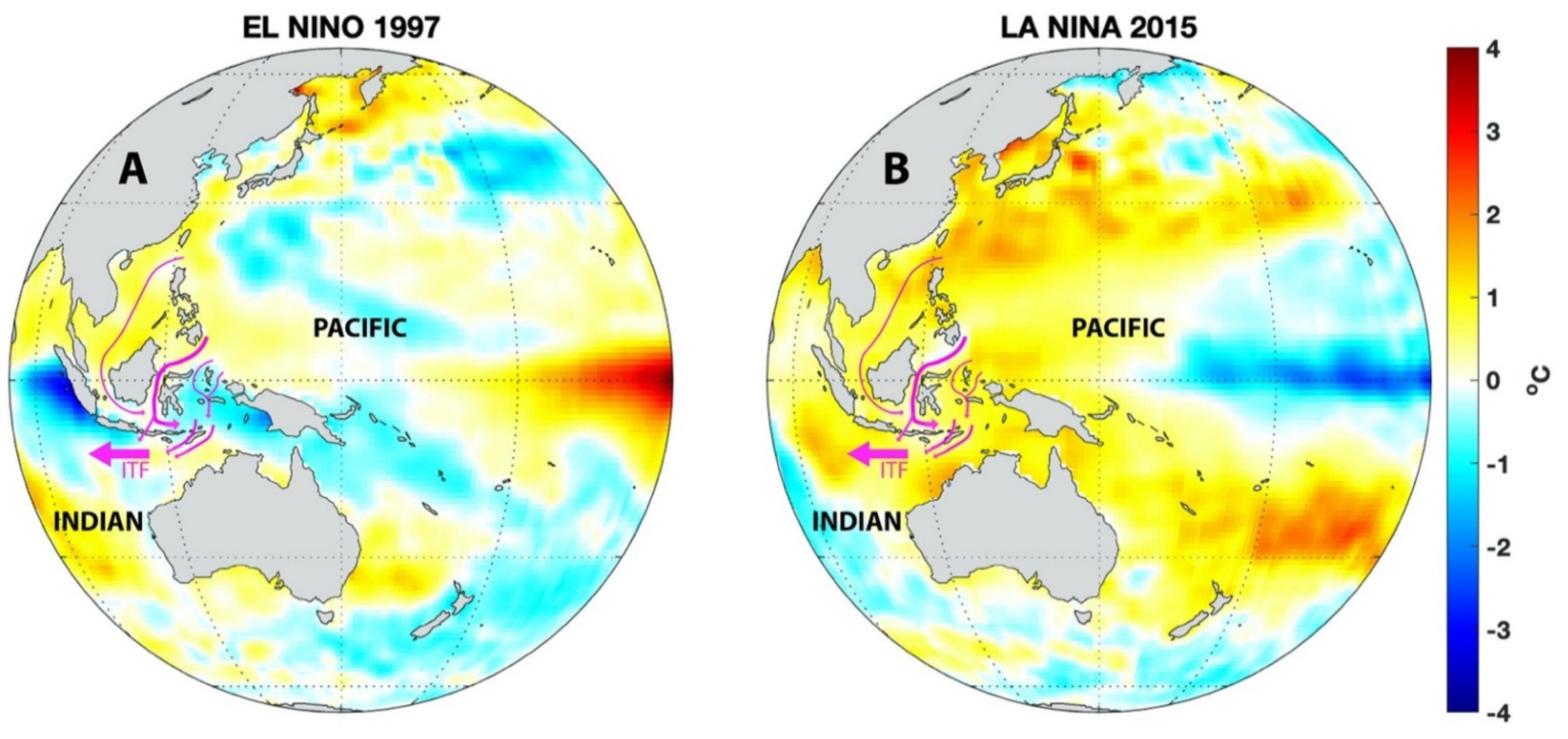
With their complex geography and narrow passages, the Indonesian seas provide the only pathway for low-latitude Pacific Ocean water to flow into the Indian Ocean (Figure 1). Transport and water-mass transformation associated with the Indonesian throughflow (ITF) directly impacts the heat and freshwater budgets of the Pacific and Indian Oceans, and influences the El Niño Southern Oscillation (ENSO) and Asian–Australian monsoons, e.g., [1,2,3]. Furthermore, the Indonesian seas are a prime location of atmospheric convection that drives the Walker Circulation. Hence any changes in sea surface temperature (SST) within these regions will have global impacts on weather and climate events, e.g., [4,5,6]. Ocean mixing in the Indonesian seas affects the mean state of the Indo-Pacific region and its interannual variability [7].
Along the ITF pathways, waters experience strong tidal mixing and air-sea interactions. The detailed geography of nonlinear interactions between tides and tidally-induced mixing, and the influence of the ITF and strait geometry in the Indonesian seas are complicated and not fully understood. The temperature and salinity stratification are significantly altered within the Indonesian Seas’ complex topography by turbulent mixing processes [2,8]. Although the core of the ITF is at about 100 m depth, the mixing drives Sea Surface Temperature (SST) changes by several °C [2]. While many aspects of the water-mass modification remain poorly understood, it is clear that tidally-driven mixing is a crucial component [2,8,9,10,11,12,13,14]. Ffield and Gordon [15] argued for tidal mixing by identifying a pronounced spring-neap tidal cycle in satellite SST data centered on the Banda Sea. A more recent satellite study by Ray and Susanto [16], based on much more superior SST measurements, produced significantly different results with the strongest fortnightly SST signals localized to relatively small straits, channels, and sills—Sulu Sill and exit passages of the Indonesian seas from Bali to the Timor Islands. The analysis of Ray and Susanto [16] identified little significant fortnightly SST signals in the central Banda Sea, which is consistent with in situ microstructure measurements of weak mixing there [17]. It also identified moderate fortnightly SST signals in Lifamatola Passage and Manipa Strait, where microstructure measurements show significant tidal mixing with dissipation rates ranging from 10−7 to 10−6 W kg−1 [18,19]. Slightly lower fortnightly SST signals are seen in the Ceram and Halmahera seas, consistent with in situ observations [8,19,20]. Meanwhile, Lombok Strait and Sape Strait show even stronger fortnightly SST signals than those regions. This is also consistent with in situ measurements [19]. Note that the fortnightly satellite SST amplitude (~0.1 °C) [16,21] should not be confused with the much larger, regional SST change of >0.5 °C described by Sprintall et al. [2]. The 0.5° change represents the time-mean effect on SST throughout the Indonesian Seas owing to the presence of ocean mixing, tidal or otherwise, and not the very localized fluctuations at the fortnightly period. The latter, however, are indisputably from tidal mixing, since only tides can induce a signal at exactly that period.
Using a numerical model that includes tides, Nugroho et al. [22] show a similar map of fortnightly variability in SST. All the mixing hotspots occur in regions that display strong M2 current velocities [23] and where the model of Nagai and Hibiya [24] predicts significant dissipation of baroclinic tidal energy.
Throughout this paper, we will use MSf as shorthand for the 14.77-days beat period between the M2 and S2 semidiurnal tides (i.e., spring-neap cycle). The long-period MSf tidal constituent has the same frequency, but it plays no role here as it is very weak [21,25]. Even when appearing as a nonlinear compound tide, MSf tidal currents are far too weak to affect stratification. Any mixing at the MSf period is the result of nonlinearity arising from the fortnightly modulations of M2 by the solar S2.
At longer periods, ocean-atmosphere dynamics of the Indo-Pacific Maritime continent are strongly affected by oceanic/atmospheric climatic processes associated with Madden–Julian Oscillation (MJO), monsoon, ENSO, and the Indian Ocean Dipole (IOD). The most substantial SST variability is associated with the Asian–Australian monsoon [5,26,27]. Stratification in this region is highly dependent on these climatic conditions, such as the phase of ENSO or the phase of the monsoon season. Any stratification changes will, of course, potentially change tidal mixing. Although previous studies have shown intense mixing occurrences within the Indonesian seas and their impacts of water mass transformation into the Indian Ocean, little effort has been made to investigate the modulation of monsoon and ENSO on tidal mixing. Our understanding of tidal mixing within the Indonesian seas has been hampered by a lack of in situ and long-term observational time series.
Here we use long-term, high-spatiotemporal resolution SST to investigate monsoon and ENSO modulation of tidal mixing within the Indonesian seas. Our previous results [16,21] primarily show the mean mixing signal. Fortunately, the SST time series are now sufficiently long that we can begin to investigate some of these monsoon and ENSO modulations, at least in regions where the mixing signal is robust.
2. Expected Tidal Mixing Frequencies in Sea Surface Temperature
The primary approach of analysis of SST for tidal mixing signature is to decompose SST time series using harmonic analysis and search for spring-neap and monthly cycles. Under an assumption that the nonlinear product (e.g., quadratic) of tidal current velocities is proportional to changes in ocean temperature due to tidal mixing, the more intense the tidal current, the colder the SST [15,16,21,28]. Suppose the temperature of a region is influenced by the interaction between two tidal constituents with combined currents:
Taking the square of this time series will generate a nonlinear term with new frequencies of , , ), and :
where A1 and A2 are the amplitudes of M2 and S2, respectively, and and are the angular frequency of M2 and S2, respectively. The lower frequency has a period of 14.77 days (fortnightly, MSf). Similarly, the square of SST time series of the diurnal luni-solar tide (K1) and diurnal lunar tide (O1) will have a modulation envelope with a period of 13.66 days (near-fortnightly signal, Mf).
The strength of semidiurnal and diurnal cycles in the region dictates the spring-neap cycle of either MSf or Mf signals. For example, Indonesian seas exhibit mostly an MSf signal while the South China Sea displays a substantial Mf signal. For some regions, such as New England’s coast, the N2 tidal constituent is larger than S2. Therefore, the square of N2 and M2 would generate a monthly tidal envelope with 27.55 days [16].
The following section discusses the harmonic analysis of SST to extract spring-neap MSf tidal signals and determine monsoon and ENSO modulations.
3. Sea Surface Temperature Data and Method
In remote sensing of SST, there are generally two types of sensors: infrared and microwave. The infrared measurements provide high spatial resolutions on the order of 1–2 km, i.e., the Multiscale Ultrahigh Resolution SST (MURSST) product [29]. These data were used by Ray and Susanto [16,21] and Susanto et al. [28] to extract tidal mixing signals in Indonesian seas and Hong Kong coastal waters, respectively. However, infrared measurements are often obstructed by clouds, which can be problematic in some regions such as Southeast Asia.
Microwave sensors provide data in nearly all weather conditions but provide considerably coarser spatial resolution on the order of 25–50 km [30]. They require a mask of 50–75 km around the land, depending on the sensor specifics, owing to the large microwave footprint and the possible contamination when land falls within the antenna sidelobes, e.g., [31].
This study uses the global daily gridded compilation from the Group for High-Resolution Sea Surface Temperature (GHRSST) [32,33]. The GHRSST products aim to achieve the best combination of these different systems, a combination of infrared and microwave sensors with a spatial resolution of 0.09° × 0.09°. The data were available from the NASA-PODAAC from June 2002 to the present [34] and were accessed on 28 July 2021.
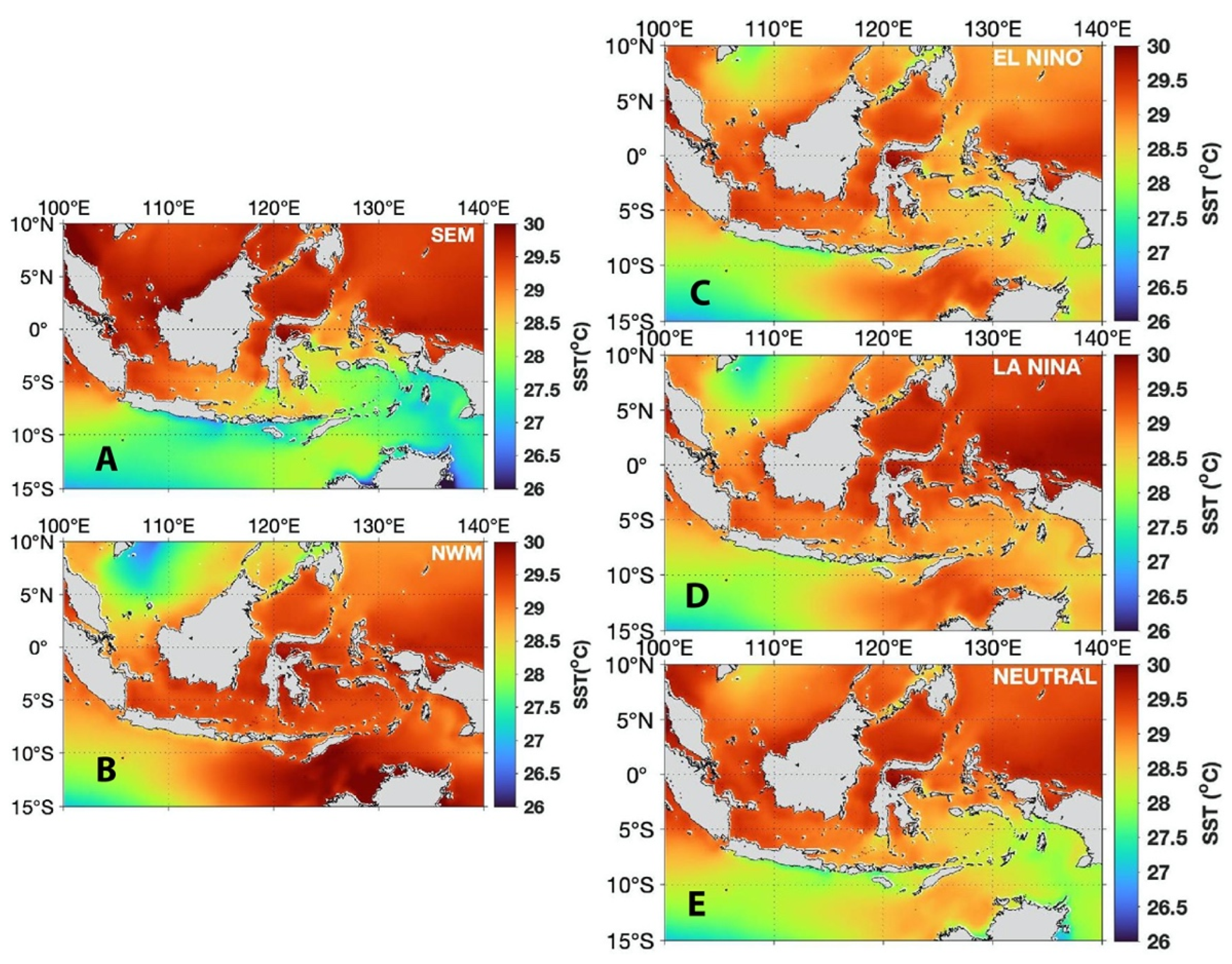
The SST time series from June 2002 to June 2021 were partitioned into segments according to the monsoon or ENSO phases, and then harmonic analysis was applied separately to each. Within the Indonesia Maritime Continent, the monsoon phase is usually defined based on the combination of annual rainfall patterns and winds, i.e., [35]. Southeast monsoon (SEM) is defined as April to September, characterized by dry air and less rainfall. Meanwhile, the northwest monsoon (NWM) is characterized by high humidity and wet conditions from October to March. For the ENSO phase, we use the Oceanic Niño Index (ONI; https://www.cpc.ncep.noaa.gov/data/indices/and accessed on 1 September 2021). El Niño defines as ONI ≥ 0.5 °C and La Niña defines as ONI ≤ −0.5 °C. Figure 2 shows an average SST from 2002 to 2017, during (a) the southeast monsoon, (b) during the northwest monsoon, (c) El Niño, (d) La Niña, and (e) Neutral year.
4. Results
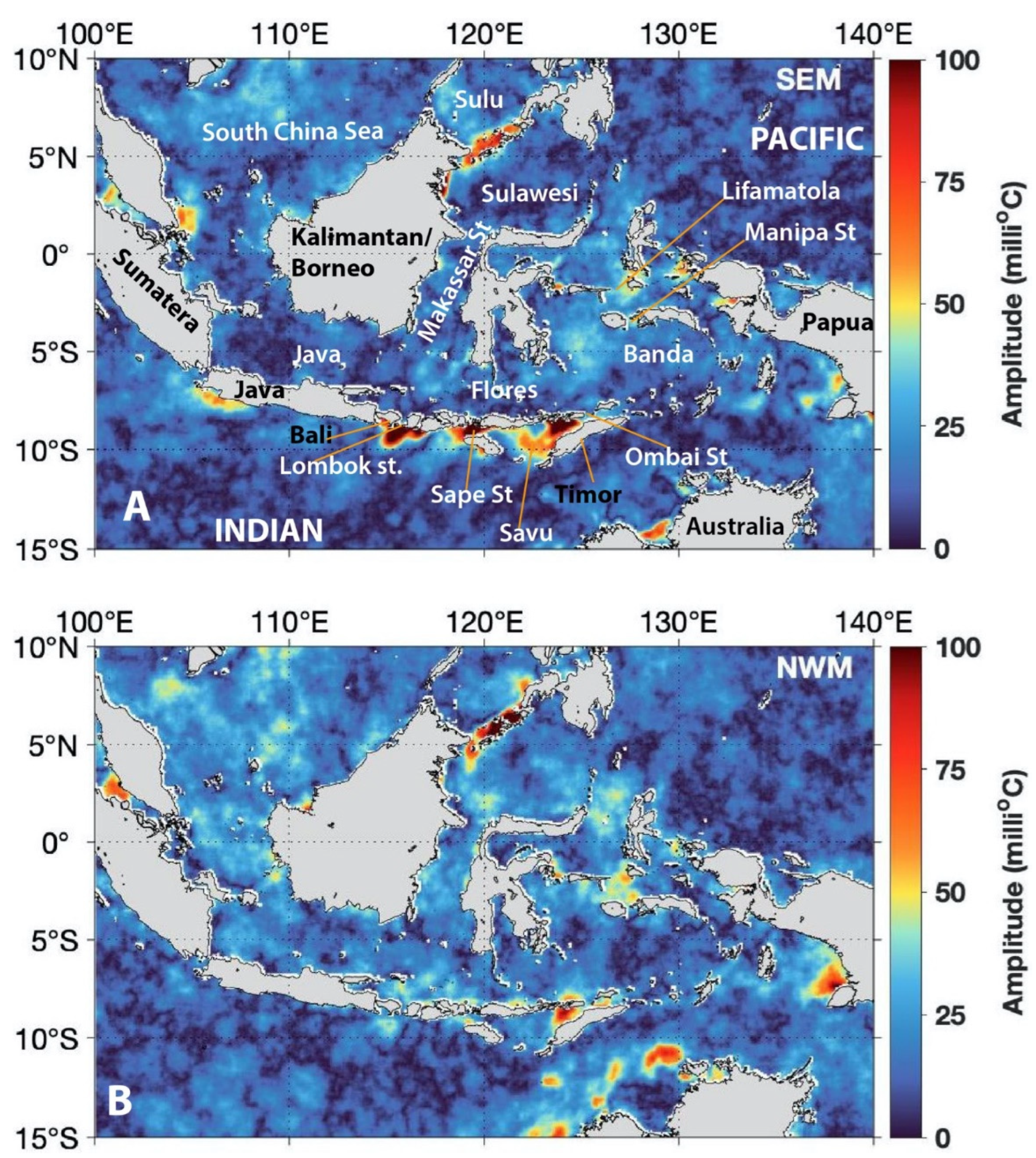
Figure 3 shows the main results of extracting 14.77-day MSf amplitude from the SST time series from June 2002 to June 2021 for the southeast monsoon (boreal summer) and northwest monsoon (boreal winter). During southeast monsoon, easterly wind-induced upwelling occurs along the southern coasts of the Lesser Sunda Island chain from Java to Timor and Banda Sea with clearly distinctive SST pattern (Figure 2A). Hence, stronger stratifications in the exit passages of ITF in the Lombok, Sape, and Ombai Straits translate to stronger mixing signatures, as seen in Figure 3A. Meanwhile, during the northwest monsoon, the westerly winds from Asia/South China Sea do not generate a distinct pattern within the Indonesia seas (except in the South China Sea). The relationship between SST, monsoonal winds, and tidal mixing has been investigated using a numerical model [27,36,37]. Their results (especially Nagai and Hibiya) [37] suggested that strong tidal mixing in the narrow tidal straits between the Lesser Sunda Islands creates a cold SST signal that propagates as baroclinic Kelvin waves along the Lesser Sunda Islands. The Ekman transport associated with monsoonal winds regulates the northward and/or southward propagation of these baroclinic Kelvin waves. Their results are consistent with our results.
Figure 3 shows stronger tidal mixing signatures during the boreal summer than in the boreal winter. The vigorous mixing locations are consistent with previous results [16]. They are primarily concentrated in the narrow exit passages of ITF into the Indian Ocean along the Lesser Sunda Island chain and Sulu Sill. Moderate mixings are observed around Halmahera/Ceram Sea, Lifamatola passage, and Manipa Strait. Meanwhile, the interior Banda Sea shows a weak mixing signature.
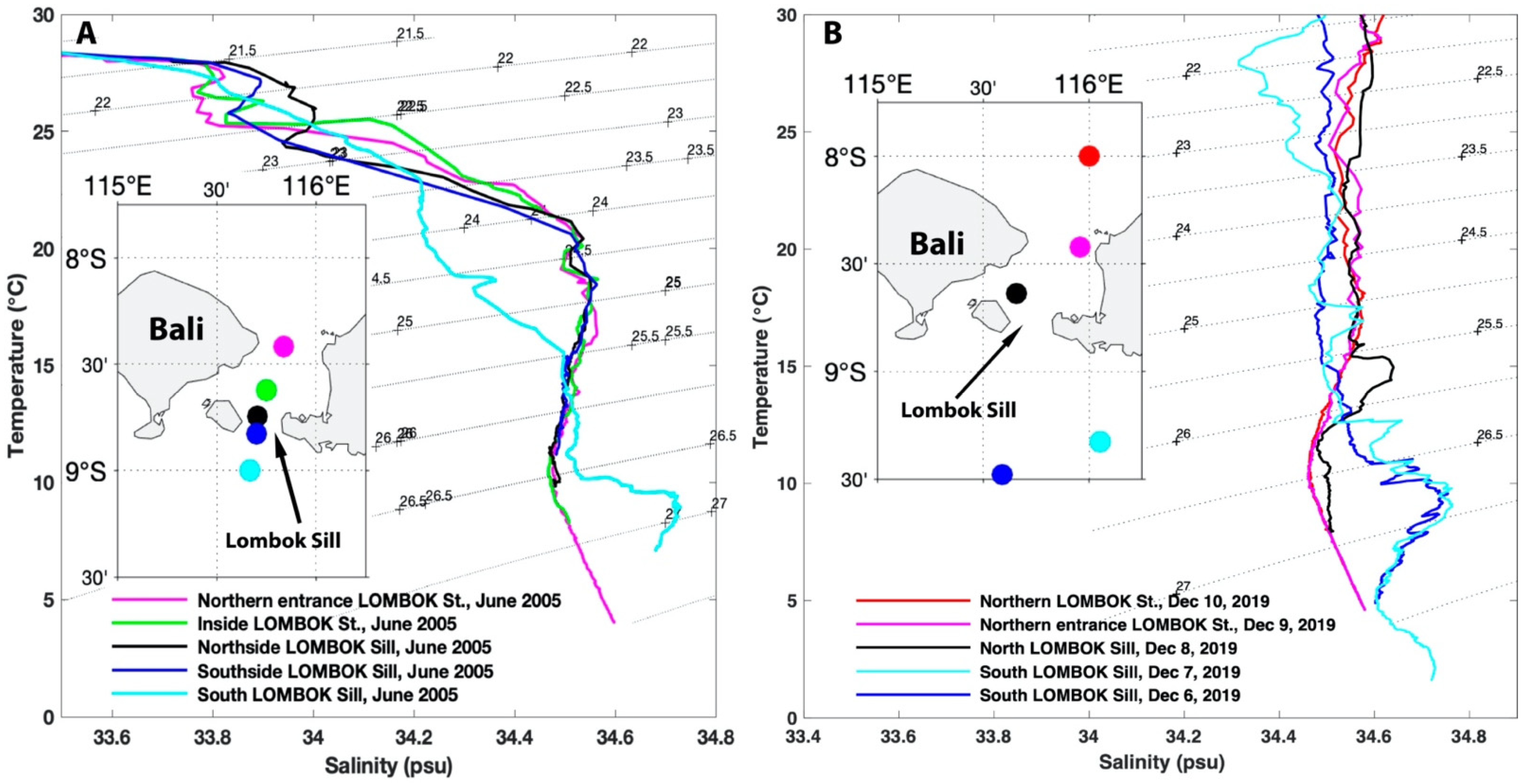
These results are consistent with in situ data of stratification based on historical Indonesian throughflow measurements of Conductivity Temperature and Depth (CTD) taken in June 2005 to represent the southeast monsoon (Figure 4A), and in December 2019 to represent the northwest monsoon (Figure 4B). The southward ITF flow of waters entering the Lombok Strait is strongest and stratified during the southeast monsoon. Along pathways in the Lombok Strait from the northern entrance to the southern side of the sill, TS profiles are nearly the same. However, when the water reaches south of Lombok Strait’s sill, the temperature-salinity (TS) properties become nearly linear, with the salinity maximum and the deeper salinity minimum mixed away, especially from σθ = 23.5 kg/m3 to σθ = 27.25 kg/m3. On the other hand, ITF southward flow to the Indian Ocean is the lowest during the northwest monsoon, even sometimes undergoing northward flow from the Indian Ocean into the Indonesian seas [38,39,40,41]. The TS properties are nearly linear from the north to the south of the Lombok Strait.
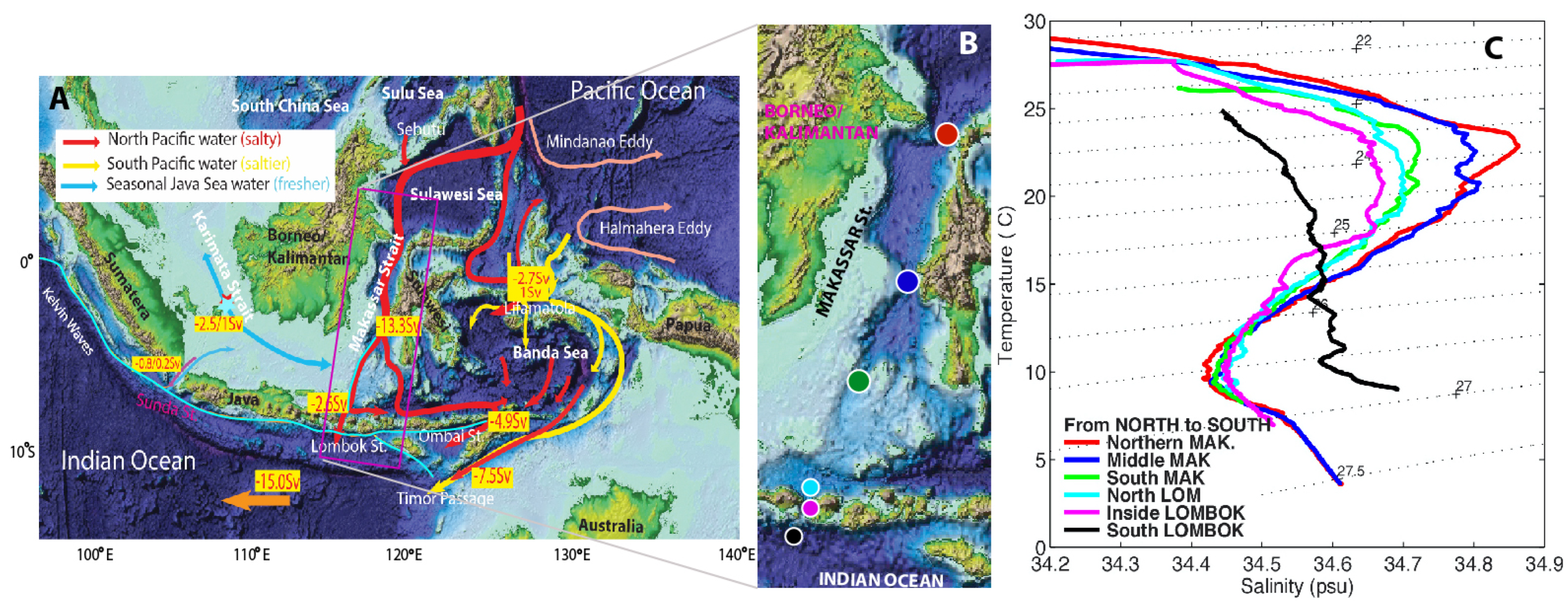
The main ITF pathway from the western Pacific enters the Sulawesi Sea into the Makassar Strait. It then splits into two pathways: the direct exit into the Indian Ocean via the Lombok Strait and the rest toward the Banda Sea (Figure 5). In situ observations show significant water-mass modification occurring in the narrow southern passages where the flow exits the Indonesian archipelago, i.e., [40]. TS curves from CTD measurements show a continual erosion of a salinity maximum centered around σθ = 24 kg/m3 from north to south through the Makassar and Lombok Straits (Figure 5B,C). Between the CTD taken in the middle of Lombok Strait and one south of Lombok Strait, the TS properties become nearly linear, with the salinity maximum and the deeper salinity minimum (centered on σθ = 26.5 kg/m3) having been mixed away. This abrupt change in water-mass properties indicates elevated mixing over the sills at the southern end of Lombok Strait. Remote sensing and numerical simulations strongly suggest that this mixing is tidally-driven [16,21,22,24].
Note that a relatively strong signature is seen in Figure 3 at the southern sill of the Sulu Sea for both seasons, but unlike the Lesser Sunda Island chain, the signature is more pronounced in the northwest season.
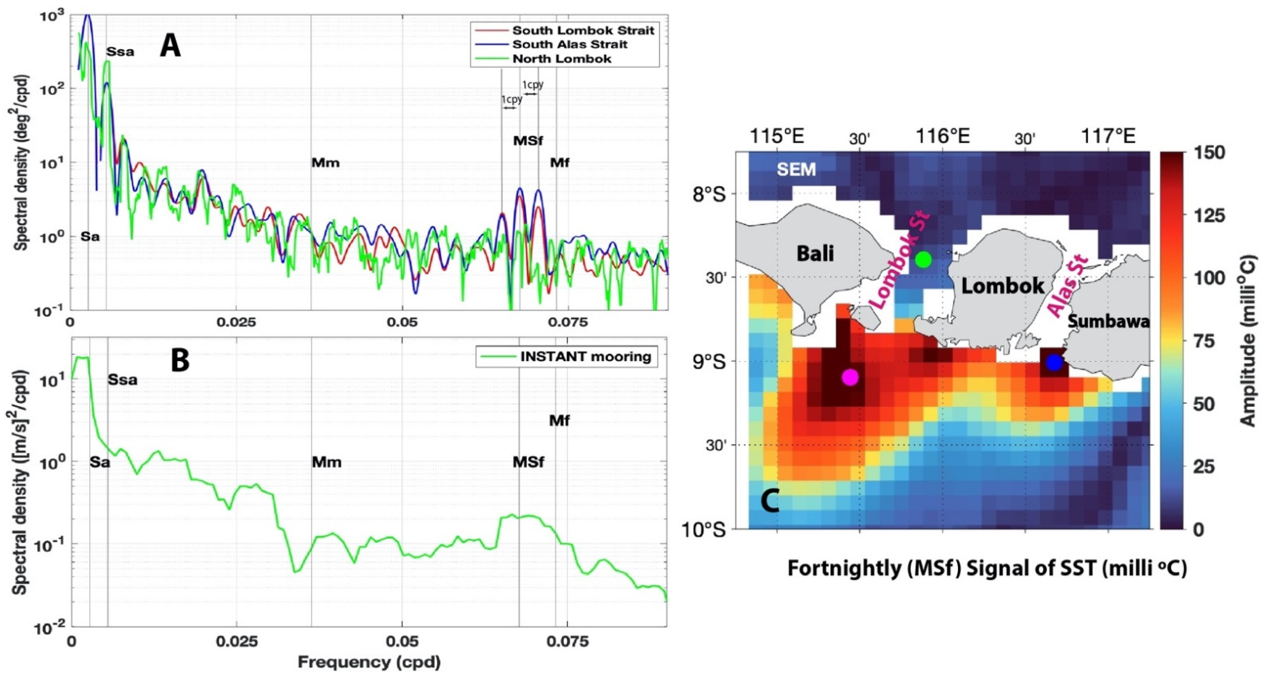
At Lombok Strait, the largest spring-neap SST amplitudes during the southeast monsoon (Figure 3A) and the annual average occur almost 75 km south of the sill. SST spectra south of Lombok and Alas Straits show narrow MSf peaks well above the background (Figure 6A). However, an SST spectrum at the northern end of Lombok Strait shows no fortnightly enhancement (green line in Figure 6A), despite there being a clear MSf signal in velocity at the INSTANT (International Nusantara Stratification and Transport) [38] mooring (Figure 6B). Aiki et al. [42] argued that the southward ITF causes the asymmetry by displacing internal tides generated at the sill southward. If southward throughflow currents are stronger than the tidal group speed at the sill, they will block propagation to the north to produce the north-south asymmetry observed in the fortnightly SST signatures. When coastal-trapped Kelvin waves propagate from the west along the south coast of Java, ITF diminishes and even reverses [43]. Figure 3B shows that the internal tide SST signature is substantially more symmetric during the northwest monsoons.
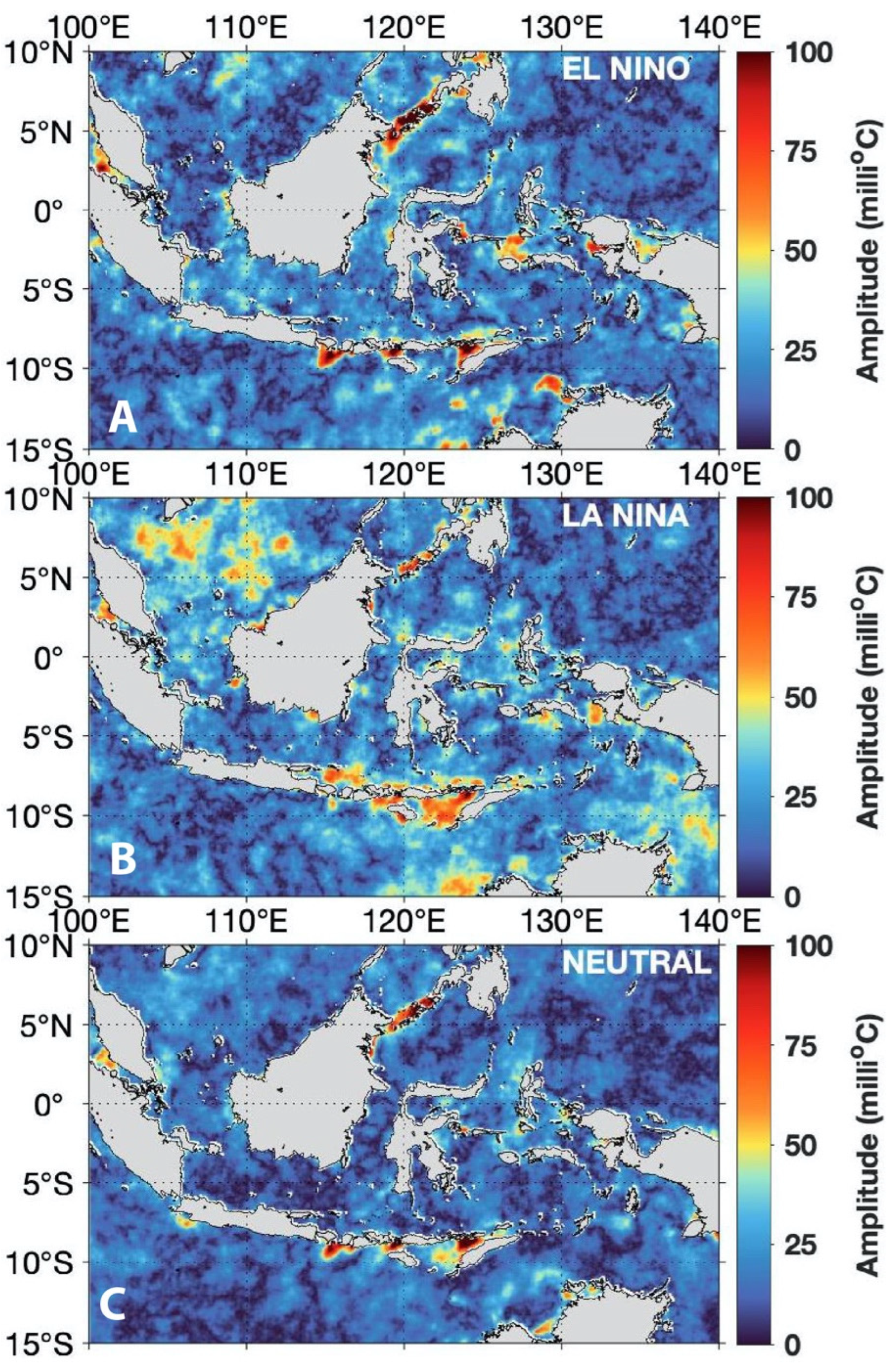
To determine the ENSO/IOD modulations of tidal mixing in the Indonesian seas, similar to our monsoon approach, we divided the SST time series into three classes, El Niño, La Niña, and Neutral, based on the ONI value of ± 0.5 °C threshold. Figure 7 shows the MSf amplitude of SST during the (a) El Niño year, (b) La Niña year, and (c) Neutral year. Figure 7 shows that the tidal mixings in the Sulu Sill and exit passages of ITF into the Indian Ocean are more vigorous during the El Niño year than during La Niña and Neutral years.
Based on Hybrid Coordinate Ocean Model (HYCOM), South China Sea throughflow is increased through the Sulu Sill during El Niño, inhibiting surface injection of tropical Pacific water into the Makassar Strait [44], and enhancing the stratification and the tidal mixing over the Sulu Sill (Figure 7). For the Lesser Sunda Island chain/exit passages of ITF into the Indian Ocean, more vigorous mixing occurs during El Niño and Neutral years, and is weaker during La Niña. Even though ITF in the Makassar Strait is weaker during El Niño and stronger during La Niña [44,45,46], ITF transport in the exit passages to the Indian Ocean remains strong during El Niño, concurrent with IOD positive. There is phase delayed of ITF transport in the outflow passage relative to the inflow passage due to ENSO variability, i.e., [47,48].
During the concurrent El Niño and IOD positive events, an anomalously strong easterly wind occurs along the southern coast of the Lesser Sunda Island chain, inducing intense upwelling, colder temperature, shallower thermocline depth, lower sea surface height, and high chlorophyll-a concentration, i.e., [39,49,50,51,52,53,54,55]. For example, prolonged anomalously early winds during concurrent El Niño 2006 and IOD events lowered sea level on the Indian Ocean side, and enhanced and extended the ITF southward flow until December 2006, i.e., [38,39,49]. This suggests that Indian Ocean dynamics may be more important than the Pacific Ocean dynamics in controlling the outflow transport and stratification during the concurrent El Niño and IOD events [13]. Therefore, these interannual events may suppress the intraseasonal and seasonal signals, and induce stronger stratification and tidal mixing signatures, as seen during the boreal summer in Figure 3A.
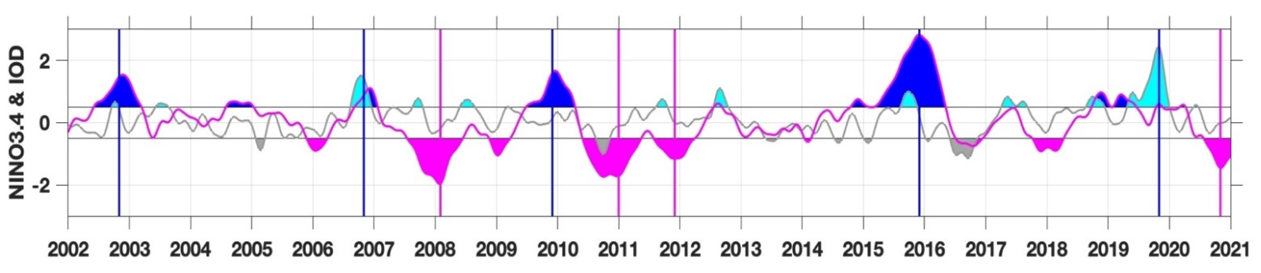
The aforementioned suggests that ENSO classification may not always be the most appropriate in all regions, e.g., [35]. Indonesian seas are affected by both ENSO and IOD events, and Indian Ocean dynamics may, at times, win over the Pacific Ocean dynamics [13]. Generally, El Niño is concurrent with IOD positive, and La Niña is concurrent with IOD negative. However, both events do not always remain in phase or perfectly aligned (Figure 8). Analysis based on IOD alone may be useful in some regions. As the SST time series continues to lengthen, we may classify the interannual variability based on IOD only and both ENSO and IOD conditions.
5. Conclusions and Discussions
With their complex geography and narrow passages, the Indonesian seas provide the only pathway for low-latitude Pacific Ocean water to flow into the Indian Ocean. Transport and water-mass transformation associated with the ITF directly impacts the heat and freshwater budgets of the Pacific and the Indian Ocean. In situ observations show extensive water-mass modification occurring in the narrow southern passages where the flow exits the Indonesian archipelago.
The influence of significant climatic phenomena associated with Southeast Asia monsoon and longer time scales associated with ENSO or Indian Ocean Dipole can be expected to affect tidal mixing in the Indonesian seas. In fact, Koch-Larrouy et al. [7] show that the interaction goes both ways: they show that mixing in the Indonesian seas affects eastern equatorial Pacific temperature and thereby affects ENSO itself.
This paper has attempted to identify monsoon and ENSO influence on tidal mixing in the Indonesian seas using high-resolution SST. The GHRSST data from 2002 to 2021 provides a map of seasonal and interannual variability of tidal mixing signatures in the Indonesian seas, which reconfirm average tidal mixing signatures derived from Multi-Ultra High-Resolution SST (MURSST) [16,21].
The most robust SST signatures are all localized to narrow straits and sills where the semidiurnal currents are very strong [23]. These regions are primarily associated with the exit passages of ITF into the Indian Ocean along the Lesser Sunda Island chain from Bali to Timor Islands, Sulu Sill, Lifamatola passage, and Manipa Strait. Most of these regions show vigorous tidal mixing during both seasons (boreal summer and winter), but boreal summer shows a stronger signal. For interannual variability, stronger tidal mixing signatures are observed during the El Niño and Neutral years, while the La Niña year shows moderate signals.
While the boreal summer finds a more significant tidal mixing signature in the Lombok Strait than boreal winter, tidal mixing signatures in the Sulu Sill are the opposite. More vigorous mixing was observed in the Sulu during boreal winter than in summer. This is consistent with remote sensing observations of tidally-induced internal waves in the two regions, i.e., [56,57]. Higher internal wave activities were observed in Sulu Sill during boreal winter than in the boreal summer, i.e., [58]. The Sebutu passage over the Sulu Sill exhibits stronger southward flow toward the Sulawesi Sea from August to December. Reversal northward flow was observed from December to July [59]. Tidally-generated solitons near exit passage sills of the Indonesian seas [14,42,56,60,61] may be responsible for the tidal mixing inferred from satellite SST. Isopycnal heaving can exceed 100 m in 6 min ([56] their Figure 3). Based on synthetic aperture radar (SAR) data, arc-like internal waves are frequently detected during boreal winter to spring when the southward throughflow is low or absent [61]. The waves may be responsible for the nearly linear stratification seen in Figure 4B. On the other hand, during boreal summer, when the southward throughflow is strongest, irregular internal waves frequently occur, which may enhance more vigorous mixing [61].
The analysis of Ray and Susanto [16], as well as the figures shown here, identified little significant fortnightly SST signal in the central Banda Sea, which is consistent with in situ microstructure measurements of weak mixing in the Banda Sea [17,19,20]. Moderate fortnightly SST signals in the Lifamatola Passage and Manipa Strait during both monsoons are consistent with in situ measurements showing intense tidal mixing with dissipation rates ranging from 10−7 to 10−6 W kg−1 [18,19]. Along the southern coasts of the Nusa Tenggara Island chain, especially south of the Lombok Strait, Sape Strait/Sumba Sea, and Alor/Savu Sea, even stronger fortnightly SST signals can be seen. Lombok Strait is collocated with the most significant water-mass changes (Figure 4A and Figure 5C). This result is consistent with in situ measurements in the Lombok Strait and Sape Strait [19].
Although there is compelling remote sensing evidence for vigorous tidal mixing along the exit passages of ITF or the Nusa Tenggara Island chain, this critical process has not been sufficiently explored with in situ observations. Nagai et al. [19] measured mixing in the Lombok and Sape Straits using a microstructure profiler, although their measurements were limited to two or three profiles at each station (ten near the Lombok Sill), so did not cover a complete spring-neap cycle as observed by Alford et al. [17] in the Banda Sea. Recently, Susanto led extensive tidal mixing measurements in collaboration with scientists from Indonesia and China in the south of the Lombok Strait for fifteen consecutive days. The data are being analyzed and will be reported in future publications. It would be ideal to use shipboard and moored observations that cover boreal summer and winter to similarly explore in more detail the underlying processes and variability. Validating these results in the Lombok Strait will open up the possibility of using remotely sensed SST data to estimate tidal mixing in other regions around the global ocean.
Author Contributions
Conceptualization, R.D.S. and R.D.R.; methodology, R.D.R.; software, R.D.S.; validation, R.D.S.; formal analysis, R.D.S. and R.D.R.; investigation, resources, data curation, R.D.S.; writing—original draft preparation, R.D.S.; writing—review and editing, R.D.R.; visualization, R.D.S.; supervision, R.D.R.; project administration, R.D.S.; funding acquisition, R.D.S. and R.D.R. All authors have read and agreed to the published version of the manuscript.
Funding
This research was funded by the NASA Physical Oceanography program: R.D.S, grant number 80NSSC18K0777 through the University of Maryland, College Park, and R.D.R by intra-agency within the NASA.
Data Availability Statement
All remotely sensed data are publicly available from the NASA-PODAAC (https://podaac.jpl.nasa.gov/) accessed on 28 July 2021, while the in situ CTD data are available upon request. The Oceanic Niño Index is https://www.cpc.ncep.noaa.gov/data/indices/ and was accessed on 1 September 2021. The Dipole Mode Index (DMI) is publicly available from https://stateoftheocean.osmc.noaa.gov/sur/ind/dmi.php and was accessed on 1 September 2021.
Acknowledgments
The authors thank the Indonesian government, especially the Agency for Marine Affairs and Fisheries (BRKP), the Indonesian Research Institute (LIPI), the Agency for Assessment and Application of Technology (BPPT), and the Marine Geological Institute (MGI) for their support on the Indonesian throughflow monitoring programs. We also thank the captain, crew, and technicians of the Indonesian Research Vessels of Baruna Jaya, the Geomarine III, and the Madidihang III for helping obtain in situ data.
Conflicts of Interest
The authors declare no conflict of interest. The funders had no role in the design of the study; in the collection, analyses, or interpretation of data; in the writing of the manuscript, or in the decision to publish the results.
References
- Bryden, H.L.; Imawaki, S. Ocean transport of heat. In Ocean Circulation and Climate: Observing and Modelling the Global Ocean; Siedler, G., Church, J., Gould, J., Eds.; This Is Volume 77 in the International Geophysics Series; Academic Press: San Diego, CA, USA, 2001. [Google Scholar]
- Sprintall, J.; Gordon, A.L.; Koch-Larrouy, A.; Lee, T.; Potemra, J.T.; Pujiana, K.; Wijffels, S.E. The Indonesian Seas and Their Role in the Coupled Ocean–climate System. Nat. Geosci. 2014, 7, 487–492. [Google Scholar] [CrossRef]
- Lee, S.-K.; Park, W.; Baringer, M.O.; Gordon, A.L.; Huber, B.; Liu, Y. Pacific Origin of the Abrupt Increase in Indian Ocean Heat Content during the Warming Hiatus. Nat. Geosci. 2015, 8, 445–449. [Google Scholar] [CrossRef]
- Barsugli, J.J.; Sardeshmukh, P.D. Global Atmospheric Sensitivity to Tropical SST Anomalies Throughout the Indo-Pacific Basin. J. Clim. 2002, 15, 3427–3442. [Google Scholar] [CrossRef]
- Halkides, D.; Lee, T.; Kida, S. Mechanisms Controlling the Seasonal Mixed-Layer Temperature and Salinity of the Indonesian Seas. Ocean. Dyn. 2011, 61, 481–495. [Google Scholar] [CrossRef] [Green Version]
- McBride, J.L.; Haylock, M.R.; Nicholls, N. Relationships between the Maritime Continent Heat Source and the El Niño-Southern Oscillation Phenomenon. J. Clim. 2003, 16, 2905–2914. [Google Scholar] [CrossRef] [Green Version]
- Koch-Larrouy, A.; Lengaigne, M.; Terray, P.; Madec, G.; Masson, S. Tidal mixing in the Indonesian Seas and its effect on the tropical climate system. Clim. Dynam. 2010, 34, 891–904. [Google Scholar] [CrossRef]
- Purwandana, A.; Cuypers, Y.; Bouruet-Aubertot, P.; Nagai, T.; Hibiya, T.; Atmadipoera, A.S. Spatial Structure of Turbulent Mixing Inferred from Historical CTD Datasets in the Indonesian Seas. Prog. Oceanogr. 2020, 184, 102312. [Google Scholar] [CrossRef]
- Ffield, A.; Gordon, A.L. Vertical Mixing in the Indonesian Thermocline. J. Phys. Oceanogr. 1992, 22, 184–195. [Google Scholar] [CrossRef] [Green Version]
- Ffield, A.; Robertson, R. Indonesian Seas Fine-structure Variability. Oceanography 2005, 18, 108–111. [Google Scholar] [CrossRef]
- Ffield, A.; Robertson, R. Temperature fine structure in the Indonesian Seas. J. Geophys. Res. 2008, 113, C09009. [Google Scholar] [CrossRef] [Green Version]
- Robertson, R. Tidal Currents and Mixing at the Instant Mooring Locations. Dyn. Atmos. Ocean. 2010, 50, 331–373. [Google Scholar] [CrossRef]
- Sprintall, J.; Gordon, A.L.; Wijffels, S.E.; Feng, M.; Hu, S.; Koch-Larrouy, A.; Phillips, H.; Nugroho, D.; Napitu, A.; Pujiana, K.; et al. Detecting Change in the Indonesian Seas. Front. Mar. Sci. 2019, 6, 257. [Google Scholar] [CrossRef]
- Purwandana, A.; Cuypers, Y.; Bouruet-Aubertot, P. Observation of Internal Tides, Nonlinear Internal Waves and Mixing in the Lombok Strait, Indonesia. Cont. Shelf Res. 2021, 216, 104358. [Google Scholar] [CrossRef]
- Ffield, A.; Gordon, A.L. Tidal Mixing Signatures in the Indonesian Seas. J. Phys. Oceanogr. 1996, 26, 1924–1937. [Google Scholar] [CrossRef] [Green Version]
- Ray, R.D.; Susanto, R.D. Tidal Mixing Signatures in the Indonesian Seas from High-Resolution Sea Surface Temperature Data. Geophys. Res. Lett. 2016, 43, 8115–8123. [Google Scholar] [CrossRef] [Green Version]
- Alford, M.H.; Gregg, M.C.; Ilyas, M. Diapycnal Mixing in the Banda Sea: Results of the First Microstructure Measurements in the Indonesian Throughflow. Geophys. Res. Lett. 1999, 26, 2741–2744. [Google Scholar] [CrossRef]
- Tan, S.; Pratt, L.J.; Yuan, D.; Li, X.; Wang, Z.; Li, Y.; Corvianawatie, C.; Surinati, D.; Sandra, A.; Bayhaqi, A. Hydraulics and mixing of the deep overflow in the LifamatolaPassage of the Indonesian seas. J. Phys. Oceanogr. 2020, 50, 2797–2814. [Google Scholar] [CrossRef]
- Nagai, T.; Hibiya, T.; Syamsudin, F. Direct estimates of turbulent mixing in the Indonesian archipelago and its role in the transformation of the Indonesian throughflow waters. Geophys. Res. Lett. 2021, 48, e2020GL091731. [Google Scholar] [CrossRef]
- Koch-Larrouy, A.; Atmadipoera, A.; van Beek, P.; Madec, G.; Aucan, J.; Lyard, F.; Grelet, J.; Souhaut, M. Estimates of Tidal Mixing in the Indonesian Archipelago from Multidisciplinary Indomix in-Situ Data. Deep. Sea Res. Part I 2015, 106, 136–153. [Google Scholar] [CrossRef]
- Ray, R.D.; Susanto, R.D. A Fortnightly Atmospheric ‘tide’ at Bali Caused by Oceanic Tidal Mixing in Lombok Strait. Geoscience Letters 2019, 6, 6. [Google Scholar] [CrossRef]
- Nugroho, D.; Koch-Larrouy, A.; Gaspar, P.; Lyard, F.; Reffray, G.; Tranchant, B. Modelling Explicit Tides in the Indonesian Seas: An Important Process for Surface Sea Water Properties. Mar. Pollut. Bull. 2018, 131, 7–18. [Google Scholar] [CrossRef] [PubMed]
- Ray, R.; Egbert, G.; Erofeeva, S. A Brief Overview of Tides in the Indonesian Seas. Oceanography 2005, 18, 74–79. [Google Scholar] [CrossRef]
- Nagai, T.; Hibiya, T. Internal Tides and Associated Vertical Mixing in the Indonesian Archipelago. J. Geophys. Res. Ocean. 2015, 120, 3373–3390. [Google Scholar] [CrossRef]
- Pugh, D.T.; Woodworth, P.L. Sea Level Science: Understanding Tides, Surges, Tsunamis and Mean Sea-Level Changes; Cambridge University Press: Cambridge, UK, 2014. [Google Scholar]
- Qu, T.; Du, Y.; Strachan, J.; Meyers, G.; Slingo, J. Sea Surface Temperature and Its Variability in the Indonesian Region. Oceanography 2005, 18, 50–61. [Google Scholar] [CrossRef] [Green Version]
- Kida, S.; Richards, K.J. Seasonal Sea Surface Temperature Variability in the Indonesian Seas. J. Geophys. Res. Ocean. 2009, 114, C6. [Google Scholar] [CrossRef]
- Susanto, R.; Pan, J.; Devlin, A. Tidal Mixing Signatures in the Hong Kong Coastal Waters from Satellite-Derived Sea Surface Temperature. Remote Sens. 2018, 11, 5. [Google Scholar] [CrossRef] [Green Version]
- Chin, T.M.; Vazquez-Cuervo, J.; Armstrong, E.M. Algorithm Theoretical Basis Document: A Multi-Scale, High-Resolution Analysis of Global Sea Surface Temperature; Version 1.3; Jet Propulsion Laboratory: Pasadena, CA, USA, 2013. [Google Scholar]
- Wentz, F.J.; Gentemann, C.; Smith, D.; Chelton, D. Satellite Measurements of Sea Surface Temperature through Clouds. Science 2000, 288, 847–850. [Google Scholar] [CrossRef] [Green Version]
- Chelton, D.B.; Wentz, F.J. Global Microwave Satellite Observations of Sea Surface Temperature for Numerical Weather Prediction and Climate Research. Bull. Am. Meteorol. Soc. 2005, 86, 1097–1115. [Google Scholar] [CrossRef] [Green Version]
- Donlon, C.; Robinson, I.; Casey, K.S.; Vazquez-Cuervo, J.; Armstrong, E.; Arino, O.; Gentemann, C.; May, D.; LeBorgne, P.; Piollé, J.; et al. The Global Ocean Data Assimilation Experiment High-Resolution Sea Surface Temperature Pilot Project. Bull. Am. Meteorol. Soc. 2007, 88, 1197–1213. [Google Scholar] [CrossRef]
- Donlon, C.; Casey, K.; Robinson, I.; Gentemann, C.; Reynolds, R.; Barton, I.; Arino, O.; Stark, J.; Rayner, N.; LeBorgne, P.; et al. The Godae High-Resolution Sea Surface Temperature Pilot Project. Oceanography 2009, 22, 34–45. [Google Scholar] [CrossRef]
- Remote Sensing Systems. MWIR Optimum Interpolated SST Data Set, Version 5.0; Physical Oceanography DAAC (PO.DAAC), Jet Propulsion Laboratory: Pasadena, CA, USA, 2017. [Google Scholar] [CrossRef]
- Aldrian, E.; Susanto, R.D. Identification of Three Dominant Rainfall Regions Within Indonesia and Their Relationship to Sea Surface Temperature. Int. J. Climatol. 2003, 23, 1435–1452. [Google Scholar] [CrossRef]
- Kida, S.; Wijffels, S.E. The impact of the Indonesian throughflow and tidal mixing on the summer time sea surface temperature in the western Indonesian seas. J. Geophys. Res. 2012, 117, C09007. [Google Scholar]
- Nagai, T.; Hibiya, T. Combined effects of tidal mixing in narrow straits and the Ekman transport on the sea surface temperature cooling in the southern Indonesian seas. J. Geophys. Res. 2020, 125, e2020JC016314. [Google Scholar] [CrossRef]
- Sprintall, J.; Wijffels, S.E.; Molcard, R.; Jaya, I. Direct Estimates of the Indonesian Throughflow Entering the Indian Ocean: 2004–2006. J. Geophys. Res. C Ocean. 2009, 114, C7. [Google Scholar] [CrossRef]
- Susanto, R.D.; Waworuntu, J.M.; Prayogo, W.; Setianto, A. Moored Observations of Current and Temperature in the Alas Strait: Collected for Submarine Tailing Placement, Used for Calculating the Indonesian Throughflow. Oceanography 2021, 34, 240–248. [Google Scholar] [CrossRef]
- Atmadipoera, A.; Molcard, R.; Madec, G.; Wijffels, S.; Sprintall, J.; Koch-Larrouy, A.; Jaya, I.; Supangat, A. Characteristics and Variability of the Indonesian Throughflow Water at the Outflow Straits. Deep. Sea Res. Part I 2009, 56, 1942–1954. [Google Scholar] [CrossRef]
- Susanto, R.D.; Wei, Z.; Adi, T.R.; Zheng, Q.; Fang, G.; Fan, B.; Supangat, A.; Agustiadi, T.; Li, S.; Trenggono, M.; et al. Oceanography Surrounding Krakatau Volcano in the Sunda Strait, Indonesia. Oceanography 2016, 29, 264–272. [Google Scholar] [CrossRef] [Green Version]
- Aiki, H.; Matthews, J.P.; Lamb, K.G. Modeling and Energetics of Tidally Generated Wave Trains in the Lombok Strait: Impact of the Indonesian Throughflow. J. Geophys. Res. 2011, 116, C3. [Google Scholar] [CrossRef] [Green Version]
- Sprintall, J.; Gordon, A.L.; Murtugudde, R.; Susanto, R.D. A semi-annual Indian Ocean forced Kelvin waves observed in the Indonesian Seas, May 1997. J. Geophys. Res. 2000, 105, 17217–17230. [Google Scholar] [CrossRef] [Green Version]
- Gordon, A.L.; Huber, B.A.; Metzger, E.J.; Susanto, R.D.; Hurlburt, H.E.; Adi, T.R. South China Sea Throughflow Impact on the Indonesian Throughflow. Geophys. Res. Lett. 2012, 39, 127. [Google Scholar] [CrossRef] [Green Version]
- Gordon, A.L.; Sprintall, J.; Van Aken, H.M.; Susanto, R.D.; Wijffels, S.; Molcard, R.; Ffield, A.; Pranowo, W.; Wirasantosa, S. The Indonesian Throughflow during 2004–2006 As Observed by the Instant Program. Dyn. Atmos. Ocean. 2010, 50, 115–128. [Google Scholar] [CrossRef]
- Susanto, R.D.; Ffield, A.; Gordon, A.L.; Adi, T.R. Variability of Indonesian Throughflow Within Makassar Strait, 2004-2009. J. Geophys. Res. Ocean. 2012, 117, C9. [Google Scholar] [CrossRef]
- Liu, Q.-Y.; Feng, M.; Wang, D.; Wijffels, S. Interannual Variability of the Indonesian Throughflow Transport: A Revisit Based on 30 Year Expendable Bathythermograph Data. J. Geophys. Res. Ocean. 2015, 120, 8270–8282. [Google Scholar] [CrossRef] [Green Version]
- Feng, M.; Zhang, N.; Liu, Q.; Wijffels, S. The Indonesian Throughflow, Its Variability and Centennial Change. Geosci. Lett. 2018, 5, 1–10. [Google Scholar] [CrossRef]
- Horii, T.; Ueki, I.; Ando, K. Coastal Upwelling Events along the Southern Coast of Java during the 2008 Positive Indian Ocean Dipole. J. Oceanogr. 2018, 74, 499–508. [Google Scholar] [CrossRef]
- Saji, N.H.; Goswami, B.N.; Vinayachandran, P.N.; Yamagata, T. A Dipole Mode in the Tropical Indian Ocean. Nature 1999, 401, 360–363. [Google Scholar] [CrossRef]
- Susanto, R.D.; Gordon, A.L.; Zheng, Q.N. Upwelling along the coasts of Java and Sumatra sand its relation to ENSO. Geophys. Res. Letters. 2001, 28, 1599–1602. [Google Scholar] [CrossRef]
- Susanto, R.D.; Moore, T.S.; Marra, J. Ocean color variability in the Indonesian Seas during the SeaWiFS era. Geochem. Geophys. Geosyst. 2006, 7, Q05021. [Google Scholar] [CrossRef]
- Susanto, R.D.; Marra, J. Effect of the 1997/98 El Niño on Chlorophyll a Variability along the Southern Coasts of Java and Sumatra. Oceanography 2005, 18, 124–127. [Google Scholar] [CrossRef]
- Siswanto, E.; Horii, T.; Iskandar, I.; Gaol, J.L.; Setiawan, R.Y.; Susanto, R.D. Impacts of Climate Changes on the Phytoplankton Biomass of the Indonesian Maritime Continent. J. Mar. Syst. 2020, 212, 103451. [Google Scholar] [CrossRef]
- Webster, P.J.; Moore, A.M.; Loschnigg, J.P.; Leben, R.R. Coupled oceanic-atmospheric dynamics in the Indian Ocean during 1997–98. Nature 1999, 401, 356–360. [Google Scholar] [CrossRef] [PubMed]
- Susanto, R.D.; Mitnik, L.; Zheng, Q. Ocean Internal Waves Observed in the Lombok Strait. Oceanography 2005, 18, 80–87. [Google Scholar] [CrossRef]
- Liu, B.; D’Sa, E.J. Oceanic Internal Waves in the Sulu–celebes Sea Under Sunglint and Moonglint. IEEE Trans. Geosci. Remote Sens. 2019, 57, 6119–6129. [Google Scholar] [CrossRef]
- Jackson, C.R.; Apel, J.R. An Atlas of Internal Solitary-Like Waves and Their Properties; Global Ocean Associates: Rockville, MD, USA, 2004. [Google Scholar]
- Qu, T.; Song, Y.T. Mindoro Strait and Sibutu Passage Transports Estimated from Satellite Data. Geophys. Res. Lett. 2009, 36, 22. [Google Scholar] [CrossRef]
- Hatayama, T. Transformation of the Indonesian Throughflow Water by Vertical Mixing and Its Relation to Tidally Generated Internal Waves. J. Oceanogr. 2004, 60, 569–585. [Google Scholar] [CrossRef] [Green Version]
- Matthews, J.P.; Aiki, H.; Masuda, S.; Awaji, T.; Ishikawa, Y. Monsoon Regulation of Lombok Strait Internal Waves. J. Geophys. Res. Ocean. 2011, 116, C5. [Google Scholar] [CrossRef]
Figure 1.
Indonesia throughflow pathways (ITF) (purple lines) overlaid with sea surface temperature anomaly in the Indo-Pacific region during (A) the 1997 El Niño and (B) the 2015 La Niña.
Figure 1.
Indonesia throughflow pathways (ITF) (purple lines) overlaid with sea surface temperature anomaly in the Indo-Pacific region during (A) the 1997 El Niño and (B) the 2015 La Niña.

Figure 2.
Average SST from June 2002 to June 2021 during (A) the southeast monsoon (boreal summer); (B) during the northwest monsoon (boreal winter); (C) El Niño; (D) La Niña, and (E) Neutral year.
Figure 2.
Average SST from June 2002 to June 2021 during (A) the southeast monsoon (boreal summer); (B) during the northwest monsoon (boreal winter); (C) El Niño; (D) La Niña, and (E) Neutral year.

Figure 3.
The amplitude of the fortnightly signal (MSf): (A) During the southeast monsoon (boreal summer) and (B) during the northwest monsoon (boreal winter). The tidal mixing signatures are more robust/stronger during the boreal summer (when the ITF is generally stronger) than that during boreal winter.

Figure 4.
(A) Temperature-Salinity diagram of the evolution of water masses from north of Lombok Strait through Lombok Strait into the Indian Ocean taken in (A) June 2005, representing southeast monsoon and (B) December 2019, representing northwest monsoon.
Figure 4.
(A) Temperature-Salinity diagram of the evolution of water masses from north of Lombok Strait through Lombok Strait into the Indian Ocean taken in (A) June 2005, representing southeast monsoon and (B) December 2019, representing northwest monsoon.

Figure 5.
(A) Map of the main ITF pathways from the Pacific to Indian Oceans (adopted from Susanto et al. [42]). Numbers denote annual mean ITF transports in each strait with negative values representing transport toward the Indian Ocean; (B) Map of the Makassar and Lombok Straits showing the location of the stations used in (C); (C) TS diagram of the evolution of water masses from north of Makassar Strait through Lombok Strait into the Indian Ocean taken during the Indonesian throughflow monitoring program, revealing vigorous mixing in Makassar and Lombok Straits for potential densities σθ = 23–27 kg m–3.

Figure 6.
(A) SST spectrum based on 20 years of daily GHRSST data south of Lombok and Alas Straits (red and blue curves), and at the location of the INSTANT mooring at the northern end of Lombok Strait (green curve). Note that the strong MSf peaks in the red and blue curves are accompanied by two side-peaks, which are precisely one cycle-per-year (cpy) from the central MSf peaks [21], thus indicating substantial annual modulation, which Figure 3 explicitly shows; (B) Velocity spectrum of the INSTANT time series. Labeled vertical dashed lines mark frequencies Mf (T = 13.66-days); MSf (T = 14.77-days), and Mm (T = 27.55-days); the two lines at the far left mark annual and semiannual frequencies (Sa and Ssa); (C) Estimates of fortnightly (MSf) SST amplitude in milli °C (zoom in Figure 3A). Locations of observations for the spectrum analysis (red, green, and blue curves).

Figure 7.
The amplitude of the fortnightly signal (MSf): (A) During El Niño year; (B) During the La Niña year, and (C) During the normal year. Tidal mixing signatures are stronger/more robust during the El Niño year, where ITF is less than in the La Niña.
Figure 7.
The amplitude of the fortnightly signal (MSf): (A) During El Niño year; (B) During the La Niña year, and (C) During the normal year. Tidal mixing signatures are stronger/more robust during the El Niño year, where ITF is less than in the La Niña.

Figure 8.
Niño3.4 index (magenta line) and Dipole Mode Index (DMI) (gray line). Values above and below 0.5 are shaded (blue for El Niño and magenta for La Niña). Shaded in cyan denotes Indian Ocean Dipole Mode (IOD) positive, while shaded in gray denotes IOD negative. Blue vertical lines denote El Niño and magenta vertical lines denote La Niña.

Publisher’s Note: MDPI stays neutral with regard to jurisdictional claims in published maps and institutional affiliations. |
© 2022 by the authors. Licensee MDPI, Basel, Switzerland. This article is an open access article distributed under the terms and conditions of the Creative Commons Attribution (CC BY) license (https://creativecommons.org/licenses/by/4.0/).
Share and Cite
MDPI and ACS Style
Susanto, R.D.; Ray, R.D. Seasonal and Interannual Variability of Tidal Mixing Signatures in Indonesian Seas from High-Resolution Sea Surface Temperature. Remote Sens. 2022, 14, 1934. https://0-doi-org.brum.beds.ac.uk/10.3390/rs14081934
AMA Style
Susanto RD, Ray RD. Seasonal and Interannual Variability of Tidal Mixing Signatures in Indonesian Seas from High-Resolution Sea Surface Temperature. Remote Sensing. 2022; 14(8):1934. https://0-doi-org.brum.beds.ac.uk/10.3390/rs14081934
Chicago/Turabian StyleSusanto, Raden Dwi, and Richard D. Ray. 2022. "Seasonal and Interannual Variability of Tidal Mixing Signatures in Indonesian Seas from High-Resolution Sea Surface Temperature" Remote Sensing 14, no. 8: 1934. https://0-doi-org.brum.beds.ac.uk/10.3390/rs14081934
Note that from the first issue of 2016, this journal uses article numbers instead of page numbers. See further details here.