
Spatio-Temporal Analysis of Sawa Lake’s Physical Parameters between (1985–2020) and Drought Investigations Using Landsat Imageries


Abstract
:
1. Introduction
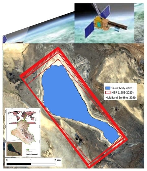
- Proposing an accurate method for estimating the length and width of lakes by implementing the so-called Minimum Bounding Rectangle (MBR) method;
- Determining the lake’s physical parameters (surface area and extent) and evaluating its changes since 1985;
- Identifying the most affected spots (i.e., spots with significant area changes);
- Estimating the growth in agricultural area around Lake Sawa and assessing their impacts on the drought of the lake.
2. Data and Methods
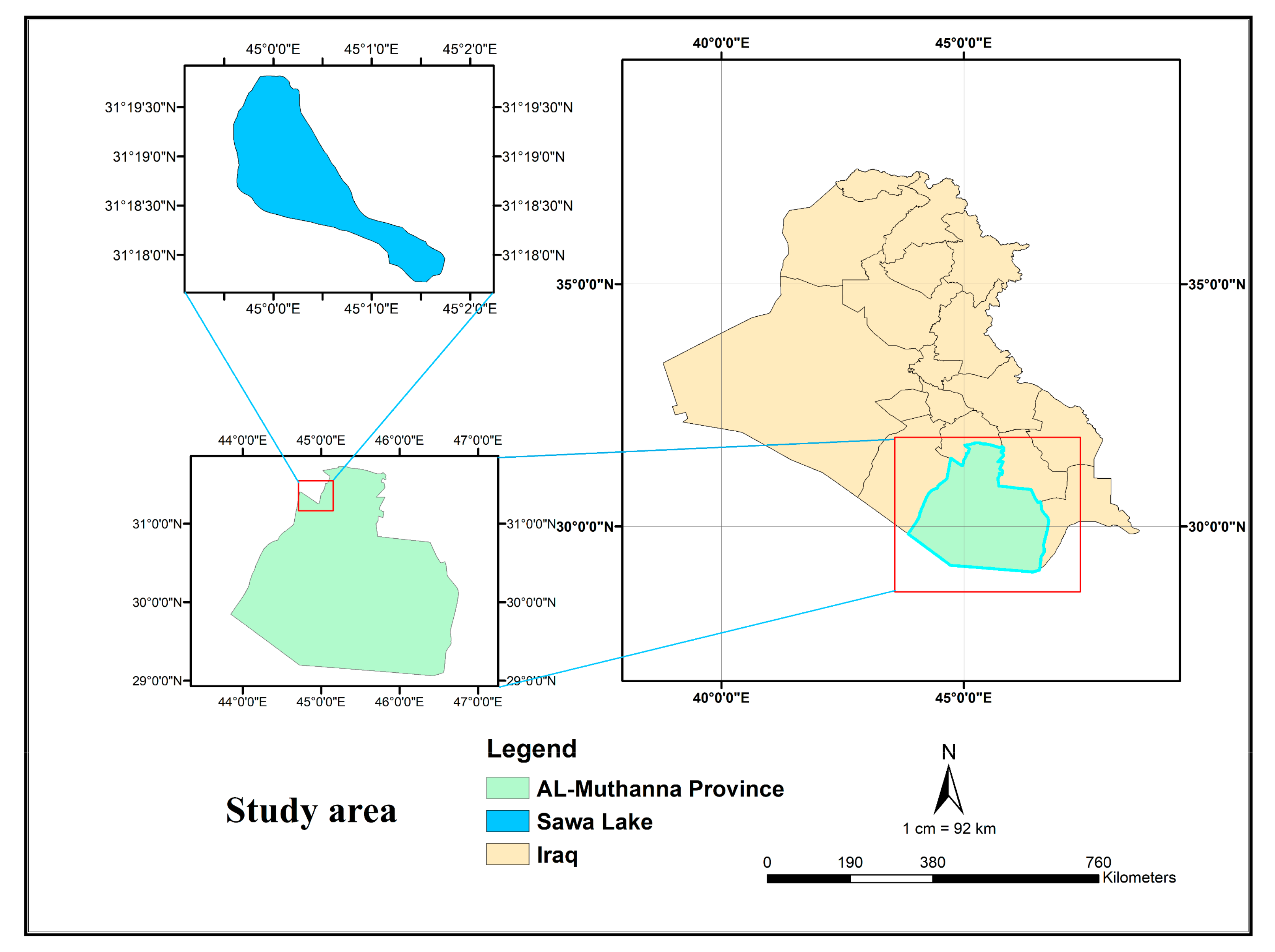
2.1. Study Area
2.2. Data
2.3. Rainfall Data
2.4. Methodology
2.4.1. Pre-Processing
2.4.2. Shoreline Extraction
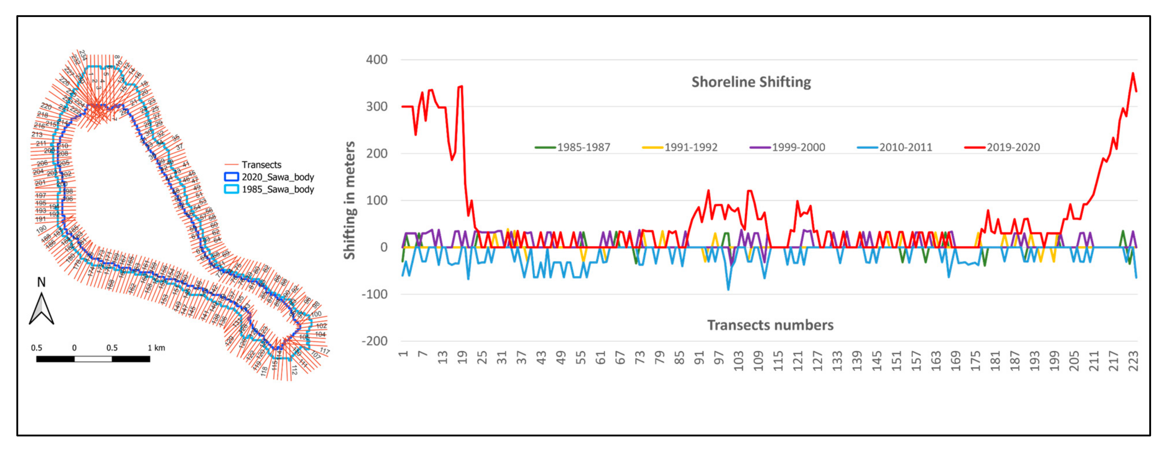
2.4.3. Shoreline Shifting
2.4.4. Agriculture Classification
2.5. Accuracy Assessment
2.5.1. Shoreline Extraction
2.5.2. Agriculture Areas
3. Results and Analysis
3.1. Lake Sawa Status
3.2. Temporal Analysis
3.2.1. Surface Area
3.2.2. Shoreline Shifting
3.2.3. MBR Length and Width
3.3. Agriculture Area
3.4. Rainfall Data Analysis
3.5. Linear Regression Analysis
4. Conclusions
Author Contributions
Funding
Acknowledgments
Conflicts of Interest
References
- Awange, J.; Saleem, A.; Sukhadiya, R.; Ouma, Y.; Kexiang, H. Physical dynamics of Lake Victoria over the past 34 years (1984–2018): Is the lake dying? Sci. Total Environ. 2019, 658, 199–218. [Google Scholar] [CrossRef] [PubMed]
- Awadh, S.M. Outstanding universal values of the Sawa Lake as a world natural heritage. Bull. Iraq Nat. Hist. Mus. 2016, 14, 1–11. [Google Scholar]
- Al-Mosawi, W.; Al-Tememi, M.; Ghalib, H.; Nassar, N. Sub-Bottom Profiler and Side Scan Sonar investigations, with the assistance of hydrochemical and isotopic analysis of Sawa Lake, Al-Muthana Governorate, Southern Iraq. Mesop. J. Mar. Sci. 2015, 30, 81–97. [Google Scholar]
- Al-Tememi, M.K.; Al-Mosawi, W.M.; Abdulnabi, Z.A. Monitoring the Change of Water Level and Its Effect on Water Quality in Sawa Lake, Southwest Iraq. Iraqi J. Sci. 2019, 2177–2185. [Google Scholar] [CrossRef]
- Deus, D.; Gloaguen, R. Remote Sensing Analysis of Lake Dynamics in Semi-Arid Regions: Implication for Water Resource Management. Lake Manyara, East African Rift, Northern Tanzania. Water 2013, 5, 698–727. [Google Scholar] [CrossRef]
- Tong, X.; Pan, H.; Xie, H.; Xu, X.; Li, F.; Chen, L.; Jin, Y. Estimating water volume variations in Lake Vic-toria over the past 22 years using multi-mission altimetry and remotely sensed images. Remote Sens. Environ. 2016, 187, 400–413. [Google Scholar] [CrossRef]
- McFeeters, S.K. The use of the Normalized Difference Water Index (NDWI) in the delineation of open water features. Int. J. Remote Sens. 1996, 17, 1425–1432. [Google Scholar] [CrossRef]
- Xu, H. Modification of normalised difference water index (NDWI) to enhance open water features in remotely sensed imagery. Int. J. Remote Sens. 2006, 27, 3025–3033. [Google Scholar] [CrossRef]
- Awange, J.; Forootan, E.; Kusche, J.; Kiema, J.; Omondi, P.; Heck, B.; Fleming, K.; Ohanya, S.; Goncalves, R. Understanding the decline of water storage across the Ramser-Lake Naivasha using satellite-based methods. Adv. Water Resour. 2013, 60, 7–23. [Google Scholar] [CrossRef]
- Feng, M.; Sexton, J.O.; Channan, S.; Townshend, J.R. A global, high-resolution (30-m) inland water body dataset for 2000: First results of a topographic–spectral classification algorithm. Int. J. Digit. Earth 2016, 9, 113–133. [Google Scholar] [CrossRef] [Green Version]
- Awange, J.; Forootan, E.; Kuhn, M.; Kusche, J.; Heck, B. Water storage changes and climate variability within the Nile Basin between 2002 and 2011. Adv. Water Resour. 2014, 73, 1–15. [Google Scholar] [CrossRef] [Green Version]
- Swenson, S.; Wahr, J. Monitoring the water balance of Lake Victoria, East Africa, from space. J. Hydrol. 2009, 370, 163–176. [Google Scholar] [CrossRef]
- Busker, T.; de Roo, A.; Gelati, E.; Schwatke, C.; Adamovic, M.; Bisselink, B.; Pekel, J.-F.; Cottam, A. A global lake and reservoir volume analysis using a surface water dataset and satellite altimetry. Hydrol. Earth Syst. Sci. 2019, 23, 669–690. [Google Scholar] [CrossRef] [Green Version]
- Awadh, S.M.; Muslim, R. The formation models of gypsum barrier, chemical temporal changes and assessments the water quality of Sawa Lake, Southern Iraq. Iraqi J. Sci. 2014, 55, 161–173. [Google Scholar]
- Ali, K.K.; Ajeena, A.R. Assessment of interconnection between surface water and groundwater in Sawa Lake area, southern Iraq, using stable isotope technique. Arab. J. Geosci. 2016, 9, 648. [Google Scholar] [CrossRef]
- Ameen, N.; Rasheed, L.; Khwedim, K. Evaluation of Heavy Metal Accumulation in Sawa Lake Sedi-ments, Southern Iraq using Magnetic Study. Iraqi J. Sci. 2019, 60, 781–791. [Google Scholar]
- Hadi, K.W. Geotechnical assessment of soil in the site of Sawa Lake Southern Iraq. EurAsian J. BioSci. 2018, 12, 27–33. [Google Scholar]
- Boschetti, T.; Awadh, S.M.; Salvioli-Mariani, E. The Origin and MgCl 2–NaCl Variations in an Atha-lassic Sag Pond: Insights from Chemical and Isotopic Data. Aquat. Geochem. 2018, 24, 137–162. [Google Scholar] [CrossRef]
- Al-Taee, A.M.; Al-Emara, E.A.; Maki, A.A. The Bacterial Fact of Sawa Lake in Samawa City Southern Iraq. Syr. J. Agrc. Res. SJAR 2018, 5, 321–328. [Google Scholar]
- Chavez, P.S., Jr. Image-based atmospheric corrections–revisited and improved. Photogramm. Eng. Remote Sens. 1996, 62, 1025–1036. [Google Scholar]
- Congedo, L. Semi-Automatic Classification Plugin: A Python tool for the download and processing of remote sensing images in QGIS. J. Open Source Softw. 2021, 6, 3172. [Google Scholar] [CrossRef]
- Saleem, A.; Dewan, A.; Rahman, M.M.; Nawfee, S.M.; Karim, R.; Lu, X.X. Spatial and temporal variations of erosion and accretion: A case of a large Tropical River. Earth Syst. Environ. 2020, 4, 167–181. [Google Scholar] [CrossRef]
- Condon, L.E.; Maxwell, R.M. Evaluating the relationship between topography and groundwater using outputs from a continental-scale integrated hydrology model. Water Resour. Res. 2015, 51, 6602–6621. [Google Scholar] [CrossRef] [Green Version]
- Benz, U.; Schreier, G. Definiens Imaging GmbH: Object oriented classification and feature detection. IEEE Geosci. Remote Sens. Soc. Newsl. 2001, 9, 16–20. [Google Scholar]
- Goodchild, M.F.; Hunter, G.J. A simple positional accuracy measure for linear features. Int. J. Geogr. Inf. Sci. 1997, 11, 299–306. [Google Scholar] [CrossRef]
- Mousa, Y.A.-K. Building Footprint Extraction from LiDAR Data and Imagery Information. Ph.D. Thesis, Curtin University, Bentley, WA, Australia, 2020. [Google Scholar]
- Mousa, Y.A.; Helmholz, P.; Belton, D.; Bulatov, D. Building detection and regularisation using DSM and imagery information. Photogramm. Rec. 2019, 34, 85–107. [Google Scholar] [CrossRef] [Green Version]
- Merkel, B.; Al-Muqdadi, S.; Pohl, T. Investigation of a karst sinkhole in a desert lake in southern Iraq. FOG-Freib. Online Geosci. 2021, 58, 85–90. [Google Scholar]


| Source | Study Period | Spatial Resolution | Temporal (Days) | Images Used | Usage | |
|---|---|---|---|---|---|---|
| Multi- spectral images | Landsat 5 | July (1985–2011) | 30 m | 16 | 21 | Lake’s parameters |
| Landsat 8 | July (2013–2020) | 30 m | 16 | 8 | Lake’s parameters | |
| Landsat 5 | March (2010–2011) | 30 m | 16 | 2 | Agricultural Zones | |
| Landsat 8 | March (2010–2020) | 30 m | 16 | 8 | Agricultural Zones | |
| Sentinel-2 | July (2020) | 10 m | 5 | 2 | Lake’s parameters |
| # | Parameter | Description | Unit |
|---|---|---|---|
| 1 | Area | The area covered by water | km2 |
| 2 | Shoreline shift | The shift (maximum) of the shoreline over time. | m |
| 3 | Length | The longest extend of the water surface area in the North–South direction based on finding the Minimum Bounding Rectangle (MBR) | m |
| 4 | Width | Like length but determining the East-West direction of the MBR | m |
| Area | MBR Width | MBR Length | ||||
|---|---|---|---|---|---|---|
| Year | (Km2) | %Change | (m) | %Change | (m) | %Change |
| 1985 | 4.88 | 1982 | 4764 | |||
| 1987 | 4.86 | −0.4 | 1978 | −0.2 | 4782 | 0.4 |
| 1988 | 4.9 | 0.8 | 1974 | −0.2 | 4764 | −0.4 |
| 1989 | 4.86 | −0.8 | 1972 | −0.1 | 4752 | −0.3 |
| 1990 | 4.88 | 0.4 | 1972 | 0.0 | 4764 | 0.3 |
| 1991 | 4.82 | −1.2 | 1968 | −0.2 | 4716 | −1.0 |
| 1992 | 4.79 | −0.6 | 1972 | 0.2 | 4734 | 0.4 |
| 1994 | 4.76 | −0.6 | 1962 | −0.5 | 4740 | 0.1 |
| 1995 | 4.85 | 1.9 | 1983 | 1.1 | 4740 | 0.0 |
| 1996 | 4.83 | −0.4 | 1978 | −0.3 | 4758 | 0.4 |
| 1997 | 4.75 | −1.7 | 1960 | −0.9 | 4722 | −0.8 |
| 1998 | 4.86 | 2.3 | 1972 | 0.6 | 4746 | 0.5 |
| 1999 | 4.75 | −2.3 | 1956 | −0.8 | 4704 | −0.9 |
| 2000 | 4.62 | −2.7 | 1936 | −1.0 | 4717 | 0.3 |
| 2001 | 4.7 | 1.7 | 1948 | 0.6 | 4741 | 0.5 |
| 2002 | 4.7 | 0.0 | 1948 | 0.0 | 4735 | −0.1 |
| 2005 | 4.72 | 0.4 | 1956 | 0.4 | 4698 | −0.8 |
| 2006 | 4.62 | −2.1 | 1929 | −1.4 | 4699 | 0.0 |
| 2007 | 4.63 | 0.2 | 1941 | 0.6 | 4698 | 0.0 |
| 2010 | 4.43 | −4.3 | 1909 | −1.6 | 4644 | −1.1 |
| 2011 | 4.65 | 5.0 | 1943 | 1.8 | 4698 | 1.2 |
| 2013 | 4.6 | −1.1 | 1943 | 0.0 | 4680 | −0.4 |
| 2014 | 4.53 | −1.5 | 1927 | −0.8 | 4668 | −0.3 |
| 2015 | 4.27 | −5.7 | 1894 | −1.7 | 4548 | −2.6 |
| 2016 | 4.26 | −0.2 | 1885 | −0.5 | 4524 | −0.5 |
| 2017 | 4.19 | −1.6 | 1866 | −1.0 | 4493 | −0.7 |
| 2018 | 4.01 | −4.3 | 1819 | −2.5 | 4397 | −2.1 |
| 2019 | 4.06 | 1.2 | 1828 | 0.5 | 4428 | 0.7 |
| 2020 | 3.58 | −11.8 | 1672 | −8.5 | 4141 | −6.5 |
| Years | Agriculture Area in Hectares | Lake Sawa Area in Hectares | Expanding of Agricultures Land in % Compared to the Previous Year |
|---|---|---|---|
| 2010 | 3799 | 442.98 | |
| 2011 | 6439 | 465.39 | 69.49 |
| 2013 | 5996 | 459.54 | −6.88 |
| 2014 | 9381 | 452.7 | 56.45 |
| 2015 | 9142 | 427.32 | −2.55 |
| 2016 | 10,482 | 425.7 | 14.66 |
| 2017 | 11,958 | 419.13 | 14.08 |
| 2018 | 11,810 | 401.22 | −1.24 |
| 2019 | 18,752 | 405.54 | 58.78 |
| 2020 | 18,059 | 358.38 | −3.70 |
Publisher’s Note: MDPI stays neutral with regard to jurisdictional claims in published maps and institutional affiliations. |
© 2022 by the authors. Licensee MDPI, Basel, Switzerland. This article is an open access article distributed under the terms and conditions of the Creative Commons Attribution (CC BY) license (https://creativecommons.org/licenses/by/4.0/).
Share and Cite
Mousa, Y.A.; Hasan, A.F.; Helmholz, P. Spatio-Temporal Analysis of Sawa Lake’s Physical Parameters between (1985–2020) and Drought Investigations Using Landsat Imageries. Remote Sens. 2022, 14, 1831. https://0-doi-org.brum.beds.ac.uk/10.3390/rs14081831
Mousa YA, Hasan AF, Helmholz P. Spatio-Temporal Analysis of Sawa Lake’s Physical Parameters between (1985–2020) and Drought Investigations Using Landsat Imageries. Remote Sensing. 2022; 14(8):1831. https://0-doi-org.brum.beds.ac.uk/10.3390/rs14081831
Chicago/Turabian StyleMousa, Yousif A., Ali F. Hasan, and Petra Helmholz. 2022. "Spatio-Temporal Analysis of Sawa Lake’s Physical Parameters between (1985–2020) and Drought Investigations Using Landsat Imageries" Remote Sensing 14, no. 8: 1831. https://0-doi-org.brum.beds.ac.uk/10.3390/rs14081831