Article

Assessing the Impacts of Tidal Creeks on the Spatial Patterns of Coastal Salt Marsh Vegetation and Its Aboveground Biomass

Ministry of Education Key Laboratory for Biodiversity Science and Ecological Engineering, National Observations and Research Station for Wetland Ecosystems of the Yangtze Estuary, School of Life Sciences, Fudan University, 2005 Songhu Road, Shanghai 200438, China
*
Author to whom correspondence should be addressed.
Submission received: 4 March 2022 / Revised: 2 April 2022 / Accepted: 8 April 2022 / Published: 11 April 2022
(This article belongs to the Special Issue Remote Sensing in Applied Ecology)

Abstract

:
The spatial distribution patterns of salt marsh plant communities and their biomass provide useful information for monitoring the stability and productivity of coastal salt marsh ecosystems in space and time. However, the spatial patterns of plant vegetation and its aboveground biomass (AGB) in a coastal salt marsh remain unclear. This study mapped the spatial distributions of salt marsh communities and their AGB based on image and LiDAR data acquired by an unmanned aerial vehicle (UAV) in the Yangtze River Estuary. The differences in vegetation structure and AGB at regions located at different distances from tidal creeks were also tested. The results show that biomass estimated through a random forest model is in good agreement (R2 = 0.90, RMSE = 0.1 kg m−2) with field-measured biomass. The results indicate that an AGB estimation model based on UAV-LiDAR data and a random forest algorithm with high accuracy was useful for efficiently estimating the AGB of salt marsh vegetation. Moreover, for Phragmites australis, both its proportion and AGB increased, while the proportion and AGB of Scirpus mariqueter, Carex scabrifolia, and Imperata cylindrica decreased with increasing distance from tidal creeks. Our study demonstrates that tidal creeks are important for shaping spatial patterns of coastal salt marsh communities by altering soil salinity and soil moisture, so reasonable and scientific measures should be taken to manage and protect coastal ecosystems.

1. Introduction

Coastal salt marshes are dominated by herbaceous plants that extend along the intertidal zone and are capable of withstanding high salinity conditions and periodic inundation because of high tides [1,2]. Salt marsh vegetation is highly productive, providing breeding, feeding, and overwintering sites for many species [3,4]. Moreover, salt marshes are recognized as critical blue carbon (C) ecosystems due to their high primary productivity, biomass regeneration rate, and C sequestration [5,6]. As a natural carbon sink, salt marsh ecosystems sequester large amounts of atmospheric carbon dioxide as standing plant biomass and peat deposits [7,8]. The estimation of aboveground biomass (AGB) is a concern in this study, for which it is closely related to aboveground carbon storage. Hence, estimating the aboveground biomass (AGB) of salt marsh vegetation offers helpful information for monitoring the stability in space and time, productivity, and aboveground carbon stocks of coastal salt marsh ecosystems [9,10]. However, previous studies on AGB estimation have been mainly limited to the site level and typically based on a single vegetation type [11,12]. The biomass density of salt marshes is variable in space, which is difficult to quantify on the landscape scale.
Both the spatial pattern and diversity of salt marsh vegetation are significantly affected by tidal flow and salinity [13,14]. Tidal flow affects the physiological ecology of plants by engineering low-oxygen and low-light conditions, and salinity directly inhibits the photosynthetic rate and respiration of salt marsh plants, which regulate the spatial structure of vegetation and growth of salt marsh plant [15]. The effect of salinity is typically parallel to that of tides, and salinity decreases with a decrease in tidal flow [16]. As almost ubiquitous features of coastal salt marsh ecosystems, tidal flow is controlled into the coastal salt marsh by tidal creeks. Tidal creeks also promote material and energy exchange between salt marshes and the outside sea through tidal fluctuations [17], which is an essential source of moisture and nutrients in soil required for the growing of salt marsh plants [18,19]. The distance from tidal creeks is related to the gradient difference of environmental factors, including tidal flow and soil salinity [20]. Therefore, the distance from the tidal creek may be an important factor that influences the distribution patterns and productivity of salt marsh vegetation. Exploring the relationship between them will improve the understanding of spatial patterns of aboveground C storage in coastal salt marshes.
Remote-sensing (RS) satellites provide advantages in spatially estimating both structural and biophysical indexes of salt marsh vegetation, particularly quantifying the biomass at lower costs, faster pace, and wider scope than the on-the-spot investigation approach [21,22]. Different RS techniques based on optical [23,24], radar [25] and LiDAR [26,27] data are widely applied to estimate AGB of coastal wetlands. However, the estimation of salt marsh AGB is restricted by the extent, spectral quality, and resolution, as well as the effects of shadows using optical sensor data. Radar data are limited by limited data availability, lack of regular and long-term coverage, data cost, and complexity of analysis [28]. LiDAR sensors have shown great potential for geometric data acquisition due to their advantages of being highly reliable and the advantage of piercing through sparse forests through repeated returns [29]. As an active RS technique, the application of unmanned aerial vehicles (UAVs) equipped with LiDAR in coastal system studies has increased over the past 10 years, including mangroves [30,31], coastal dunes [32,33], and seagrass beds [34]. UAV-LiDAR data can raise the survey and estimation of productivity and biomass in coastal salt marshes due to its advantages in providing higher spatial and temporal resolution [35,36] and have become an affordable and cost-efficient tool to map salt marsh quickly. For example, the UAV-LiDAR data can be applied for retrieving the height of plant canopy and estimating AGB, overcoming the disadvantages of satellite-based RS data [37]. Thus, it may have great potential in monitoring salt marsh three-dimensional structures in coastal wetlands [38]. However, to date, few studies have employed UAV-LiDAR data for the estimation of the AGB of salt marsh vegetation [39]. A general method with high efficiency and high precision must be constructed to estimate the whole salt marsh vegetation AGB.
To determine the impact of tidal creeks on the spatial distribution of vegetation communities and their biomass in a coastal salt marsh, this study quantifies the impact of tidal creeks on spatial patterns of a salt marsh and its AGB in a coastal wetland under primary succession in Chongming Dongtan of the Yangtze River Estuary. The purposes of this study are the following: (1) exploring the potential of applying UAV-LiDAR data in estimating salt marsh vegetation’s AGB; (2) detecting how tidal creeks shape the spatial patterns of a salt marsh plant community and its aboveground carbon storage.

2. Materials and Methods
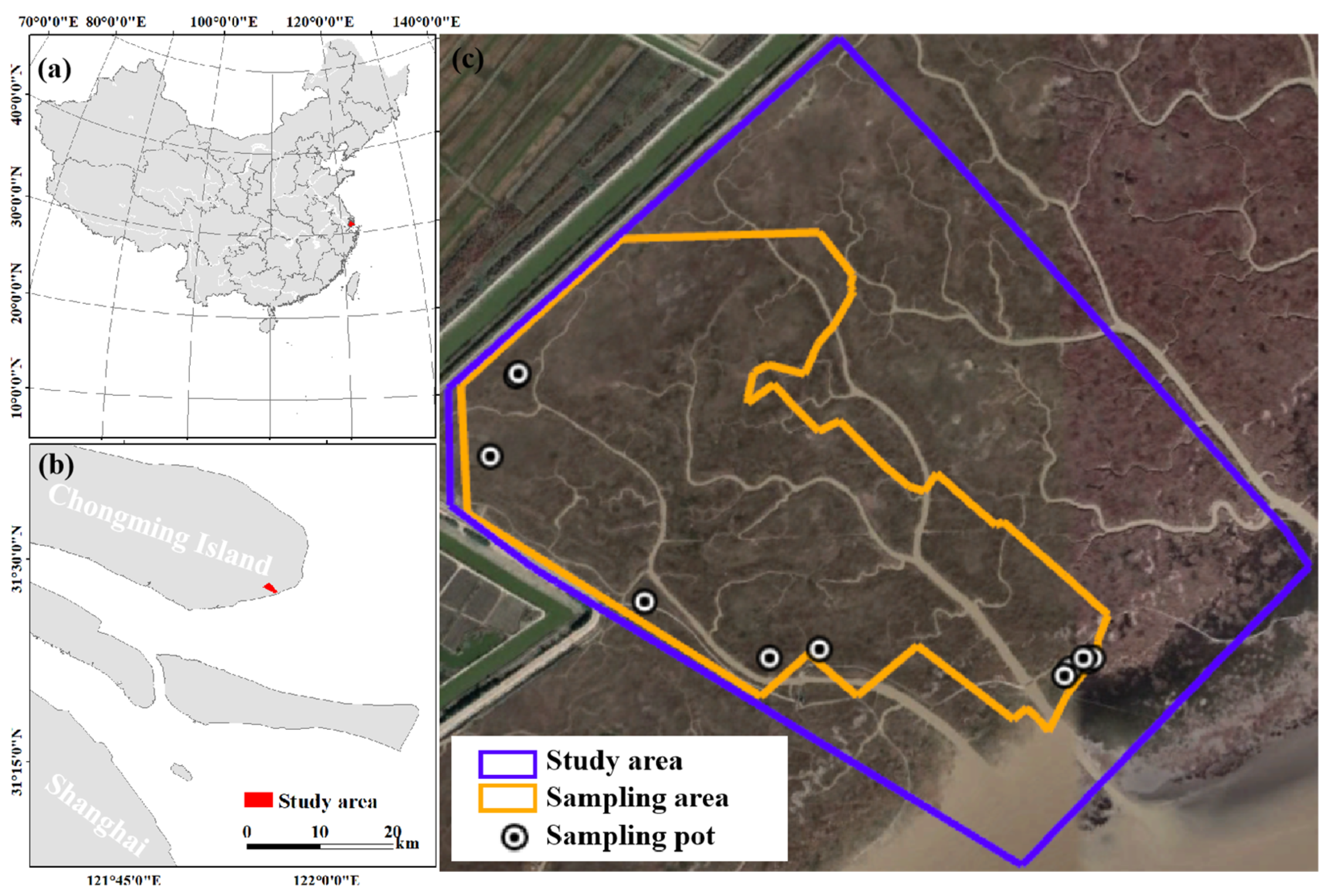
2.1. Study Area

The study area is situated in Chongming Dongtan wetland (121°54′–121°55′E, 31°27′–31°28′N) (Figure 1), located on the eastern end of Chongming Island along the Yangtze River Estuary in China. The Yangtze River Estuary is one of the principal distribution regions of coastal wetland China [39]. The study area has a total area of 0.766 km2. It is dominated by a northern subtropical monsoon climate. The annual average temperature is 15 °C, and the annual average precipitation is 102.2 cm [40]. Many tidal creeks are formed on the tidal flat in the south of Chongming east beach [41], where the intensity of human activities is relatively low. The study area experiences irregular semi-diurnal tides with an average tidal range of 2.0–3.1 m and a maximum tidal range of 4.6–6.0 m [42].
The study area is a typical muddy tidal salt marsh in the Yangtze River estuary [43]. The main plant groups include Phragmites australis and Scirpus mariqueter [44], and there is a large area of Scirpus triqueter [45]. It was found that Carex scabrifolia frequently appeared in the study area, and Imperata cylindrica also developed into a dominant species in some areas. The study area contained the entire watershed of tidal channels that affected the sampling area, and the sampling area excluded the influence of artificial rivers.

2.2. Data Collection

2.2.1. Vegetation Sampling Data Acquisition

Vegetation sampling collection in the study area was carried out in October 2019 and October 2020. We selected 20 sampling points, and each sampling point collected 3 sets of samples as parallel samples. In total, sixty 1 m × 1 m sampling plots were selected to investigate the plant species and the number of counts (Table 1). Ten individual plants from each plot were randomly selected for height measurement, and the average value was recorded as the plant height of the plot. The aboveground parts of a plant for each plot were harvested and taken to a laboratory for further processing. We dried all harvested plant samples at 50 °C in ovens to dry weights, which were regarded as the AGB values for the plots, respectively.

2.2.2. LiDAR and Optical Image Data Acquisition

UAV-LiDAR data were collected using the LR1601-IRIS LiDAR sensor based on the DJI M600 platform in September 2019. The DJI M600 UAV platform installed the LR1601-IRIS LiDAR point cloud data acquisition system, which was used to capture raw data of UAV-LiDAR. Twenty-three flight track lines were conducted, covering the 0.766 km2 study area. The ground control station was used to set the relative altitude of the flight to maintain a height of 100 m. The speed of the UAV was fixed to 1 m s−1, while the overlapping air belts were set to 30%. The scanning frequency was 320,000 Hz, the scan field angle was 360° × 30° and the velocity measurement precision was 0.03 m s−1.
The optical image data were collected using DJI Phantom 4 Pro as a data acquisition platform on 27 and 28 September 2019. The flight altitude was 120 m above the ground, the airspeed was set to 10 m per second, and the image overlap was set to 75%.

2.2.3. Soil Analysis

Soil sample data collection in the study area was carried out near each vegetation sampling point in October 2019 and October 2020. A cylindrical mud sampler with a diameter of 5 cm and a length of 30 cm was used to sample vertically on the ground. Three groups of samples were collected as parallel samples at each sampling point. The difference in sample weight (10 g) before and after heating in an oven at 105 °C for 48 h was measured to calculate soil water content. To measure soil salinity, an appropriate amount of dried soil samples and ultrapure water were dissolved according to a mass ratio of 1:5. We used a conductivity meter to measure the conductivity of the supernatant and then calculated the soil total salt content of each sample according to the conductivity measured. We randomly selected 20 samples to measure the quality of the crystals obtained after drying 50 g of the sample precipitate.

2.3. Data Preprocessing

2.3.1. UAV Image Processing and Vegetation Community Mapping

The UAV optical image was further processed using DJI Terra software to align photos and generate a dense point cloud, grid, texture, and orthophoto images, resulting in an RGB image with a resolution of 5 cm. The RGB image was used to generate training samples by visual interpretation. Fifty samples for each plant type were obtained through field investigation and visual interpretation. Seventy percent of all samples were used as the training set, and thirty percent of all samples were used as a validation set for further supervised classification.
The SV-1 20180805 images of the study area were used to conduct the boundary ruling, geometric correction, radiometric correction, and other data preprocessing on ENVI and ArcGIS software. The classification of salt marsh vegetation was completed using supervised classification based on the training samples generated by field investigation and visual interpretation.
For accuracy evaluation of vegetation classification, Kappa, overall accuracy, producer, and user accuracy were selected. The following lines are a brief description of the accuracy metrics.
The overall accuracy is a measure of the accuracy of the whole image, which is the total number of samples of correct classification divided by the total number of samples [46]. The Kappa coefficient is an index for consistency check. It can measure the effect of classification or segmentation as an index that improves overall accuracy [47]. User accuracy measures the number of samples classified correctly of a specific category divided by the total number of samples classified as that category. It is an indicator to measure the accuracy of a single category and the commission’s error [48]. Producer accuracy is the number of samples being correctly classified for a specific category divided by the total number of reference samples for that category. It measures the omission’s error [49].

2.3.2. LiDAR Data Processing

All UAV-LiDAR point cloud data were obtained using the Point Cloud Producer software. All acquired point cloud data were preprocessed under the LiDAR 360 platform for multi-strip splicing, denoising, and ground point classification to form DEM (digital elevation model) and DSM (digital surface model), and the difference between the DSM and DEM resulted in a canopy height model. Finally, ArcGIS 10.5 software was used to calculate the generated canopy height model, which has a spatial resolution of 0.05 m to obtain the average height value, the square value of the mean height, and the logarithm value of the average height with a spatial resolution of 1 m.

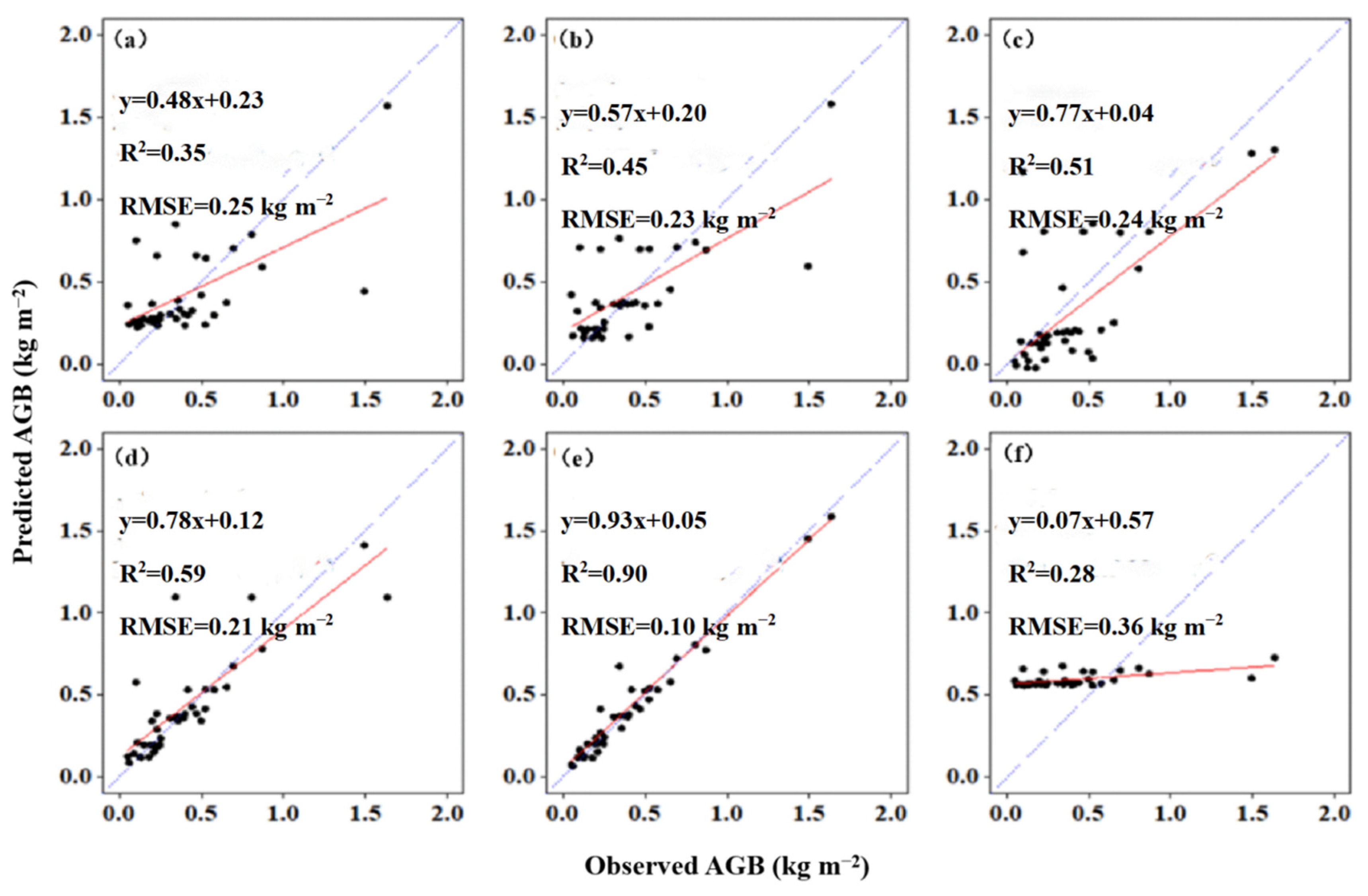
2.4. Establishment of AGB Prediction Model

In this study, all samples of salt marsh vegetation communities were used to establish a prediction model. We randomly divided all samples of salt marsh vegetation into two groups. The training set consists of seventy percent of the total number of samples, and the validation set consists of 30 percent of the total number of samples. Considering that the AGB of salt marsh vegetation has a high correlation with its canopy height [12], the average height (H), the derived factors H2 and logH of salt marsh vegetation within a 1 m2 square were also selected as predictive variables, and the AGB of salt marsh vegetation within 1 m2 was used as the dependent variable.
To find the most applicable prediction model, one linear regression model (multiple linear regression, MLR) and five machine-learning regression models, including generalized linear model (GLM), gradient boosting machine (GBM), artificial neural network (ANN), kernel-based regularized least squares (KRLS), and random forest regression (RFR), were applied to establish predicted models. Both the R2 and RMSE were applied to estimate the performance of these models and the precision of the prediction results based on the best model. The establishment and evaluation of the models were carried out in “mlr”, “gbm”, “neuralnet”, “KRLS” and “randomForest” packages of R software, respectively.
A brief description of the methods adopted in our study is as follows. MLR includes figuring out the best-fitting surface of the appropriate function form related to the value of explanatory variables, and the mean value of a response variable. Regression modeling is used to determine whether a response variable and its explanatory variables are related and to predict the value of the response variable, corresponding to the known value of the selected sub-collection of explanatory variables [50].
The generalization of linear regression is GLM, in which the difference between the error distribution model and the normal distribution of the response variables is allowed, and uses some combinations of linear, quadratic, and cubic terms to fit the parameter terms [51]. The “Poisson” regression was used in the present study because it resulted in the best fit of the logarithmic model of variables.
GBM is a novel technique that uses machine-learning techniques to construct the model and extend it by allowing the optimization of the loss function [52].
The structure of ANN consists of large amounts of neurons composed of interconnected units. It includes a large number of weighted synapses, an adder, and an activation function [53].
KRLS is an online sparse regression method based on a kernel machine. In this way, an online learning support vector machine with a sparse support vector, a small amount of calculation, and high precision can be realized [54].
The RFR consists of growing trees and depends on a random vector, so the tree predictor takes on numerical values as opposed to class labels [55]. RFR represents the complicated relation between a response variable and a set of explanatory variables. It has the ability of robustness to reduce overfitting, higher accuracy, the advantage of determining the weight of variables, low sensitivity to parameter adjustment, fewer parameters to be adjusted, and noise resistance [56].

2.5. Data Analysis

In the whole study area, we set up four buffer areas of tidal creeks at equal distance: 50 m, 100 m, 150 m and 200 m. Different distances from the tidal creeks were used to represent the different impact levels. The distance between the salt marsh vegetation community and the tidal creek was divided into four categories: 0~50 m (D1), 50~100 m (D2), 100~150 m (D3), and 150~200 m (D4). One-way variance analysis (ANOVA) was applied to check whether there were significant differences in salt marsh AGB, soil salinity, and soil moisture between different distance gradients, respectively. All the above data analysis was conducted using the R software.

3. Results

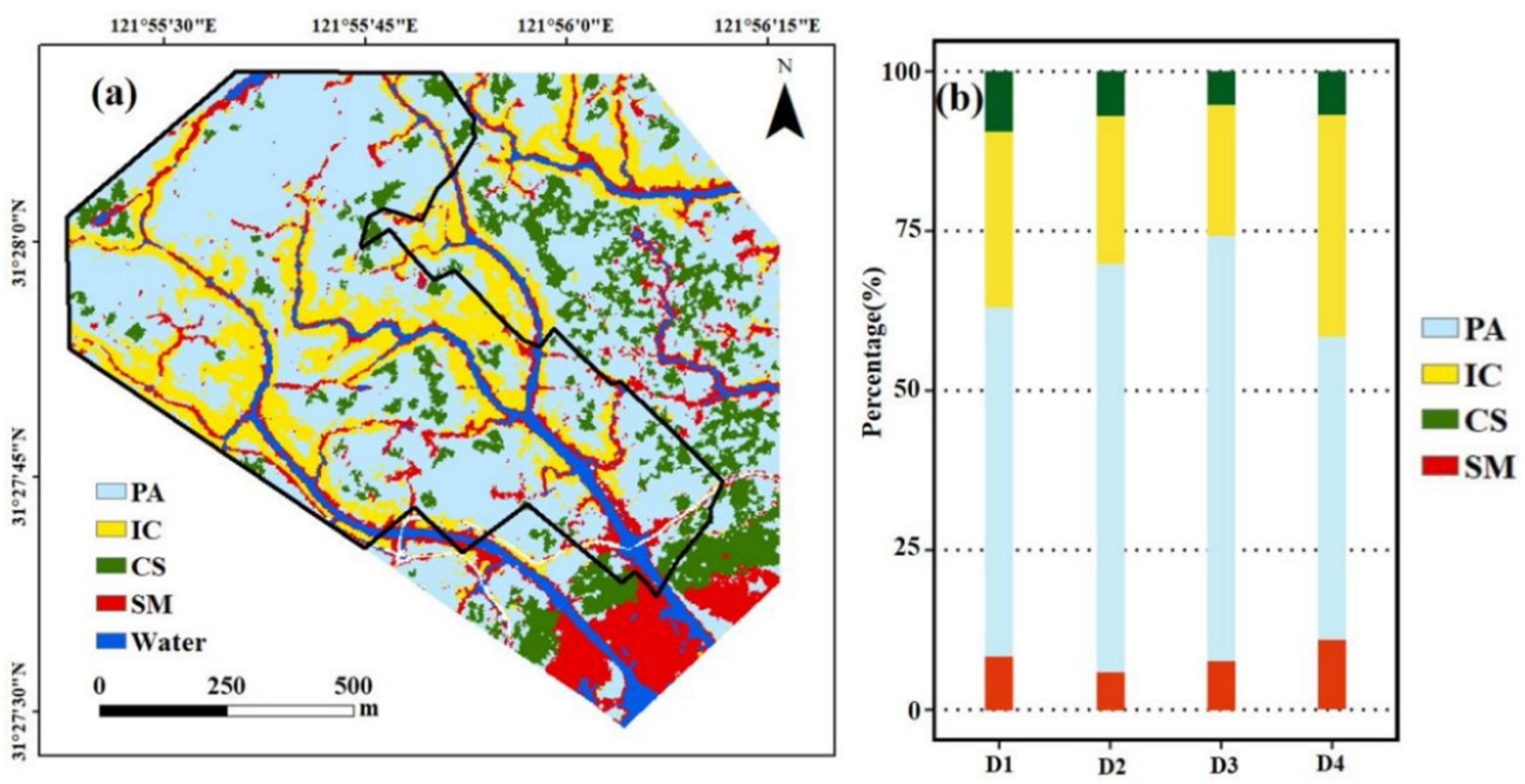
3.1. Accuracy Assessment of the Spatial Distribution of Salt Marsh Communities

Table 2 shows the results of the accuracy assessment regarding the RS classification of salt marsh communities. The producer accuracies of PA, IC, SM, and CS were 97.07%, 79.17%, 99.88%, and 96.46%, respectively, while the user accuracies were 96.89%, 98.88%, 95.15%, and 98.93%, respectively. The overall accuracies (OA) were 0.95, and the Kappa coefficients were 0.93.
Figure 2a shows the most abundant species in vegetation communities. Spatially, IC and SM were continuous distribution and appeared aggregated distribution along tidal creeks, and PA was mainly distributed within the inland domain of the research area, and CS was scattered or mixed with PA in the research area (Figure 2a). As distances from tidal creeks increased, the percentage of PA gradually increased, while other plant communities showed a downward trend (Figure 2b). Within the distance of D1 from the creeks, PA was present in the largest proportion (54.73%), followed by IC (27.68%) and CS (9.33%), while SM was present in the lowest proportion (8.26%). The largest proportion in D2 is PA (63.96%), followed by IC (23.25%), CS (6.92%), and SM (5.87%). Within the distance of D3, the proportion of PA (66.70%) was highest, compared with IC (20.58%), SM (7.62%), and CS with the lowest proportion (5.10%). The percentage of PA was the highest (47.71%) around D4 compared with the other communities—34.63%, 10.84% and 6.82% for IC, SM, and CS, respectively.

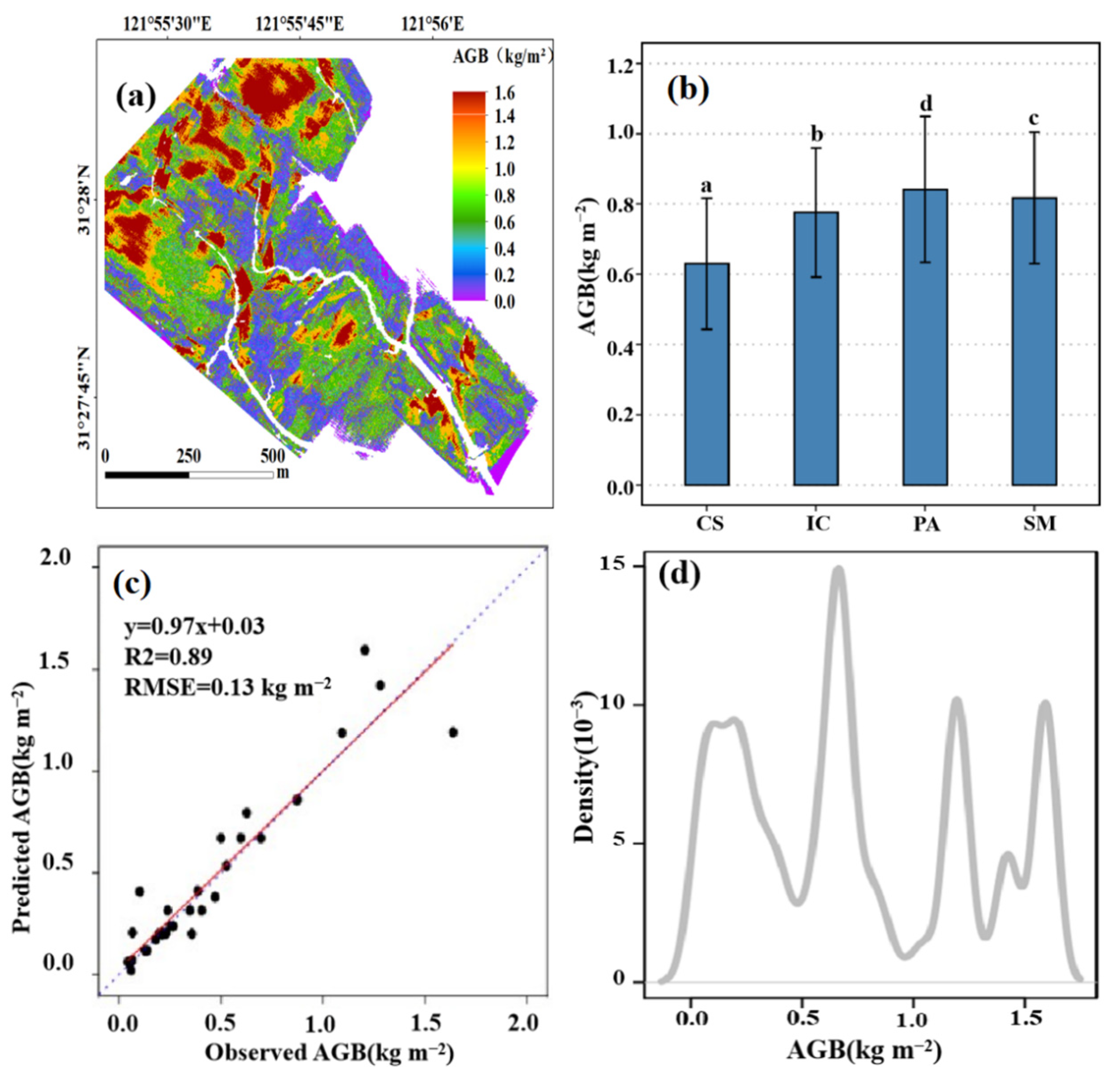
3.2. Estimation of Salt Marsh AGB and Its Spatial Pattern

The performance of the RFR (R2 = 0.90, RMSE = 0.09 kg m−2) was higher than that of the MLR model (R2 = 0.35, RMSE = 0.25 kg m−2) and that of other machine learning models in fitting salt marsh AGB with plant height, including KRLS (R2 = 0.45, RMSE = 0.23 kg m−2), ANN (R2 = 0.51, RMSE = 0.24 kg m−2), GBM (R2 = 0.59, RMSE = 0.21 kg m−2), and GLM (R2 = 0.28, RMSE = 0.36 kg m−2) (Figure 3). In particular, the RFR algorithm performed best among all machine learning models.
The best-fitted model, RFR, was applied to map the distribution of salt marsh AGB based on the height data derived from UAV-LiDAR (Figure 4a), and there was high consistency (R2 = 0.89, RMSE = 13 kg m−2) between fitted AGB and observed AGB throughout the study area (Figure 4c). The majority of the salt marsh AGB was concentratively distributed around 0.24 kg m−2, 0.67 kg m−2, 1.20 kg m−2, and 1.60 kg m−2. In particular, the AGB with a value of 0.67 kg m−2 had the highest distribution frequency. Spatially, high AGB values were mainly distributed in areas far away from the sea and tidal creek, while low AGB value pixels were mainly near the tidal creek. The mean AGB values for various salt marsh communities were significantly (p < 0.05) different from each other. In particular, the mean AGB of PA was approximately 0.87 kg m−2 and significantly (p < 0.05) higher than IC (0.74 kg m−2), SM (0.69 kg m−2), and CS (0.59 kg m−2).

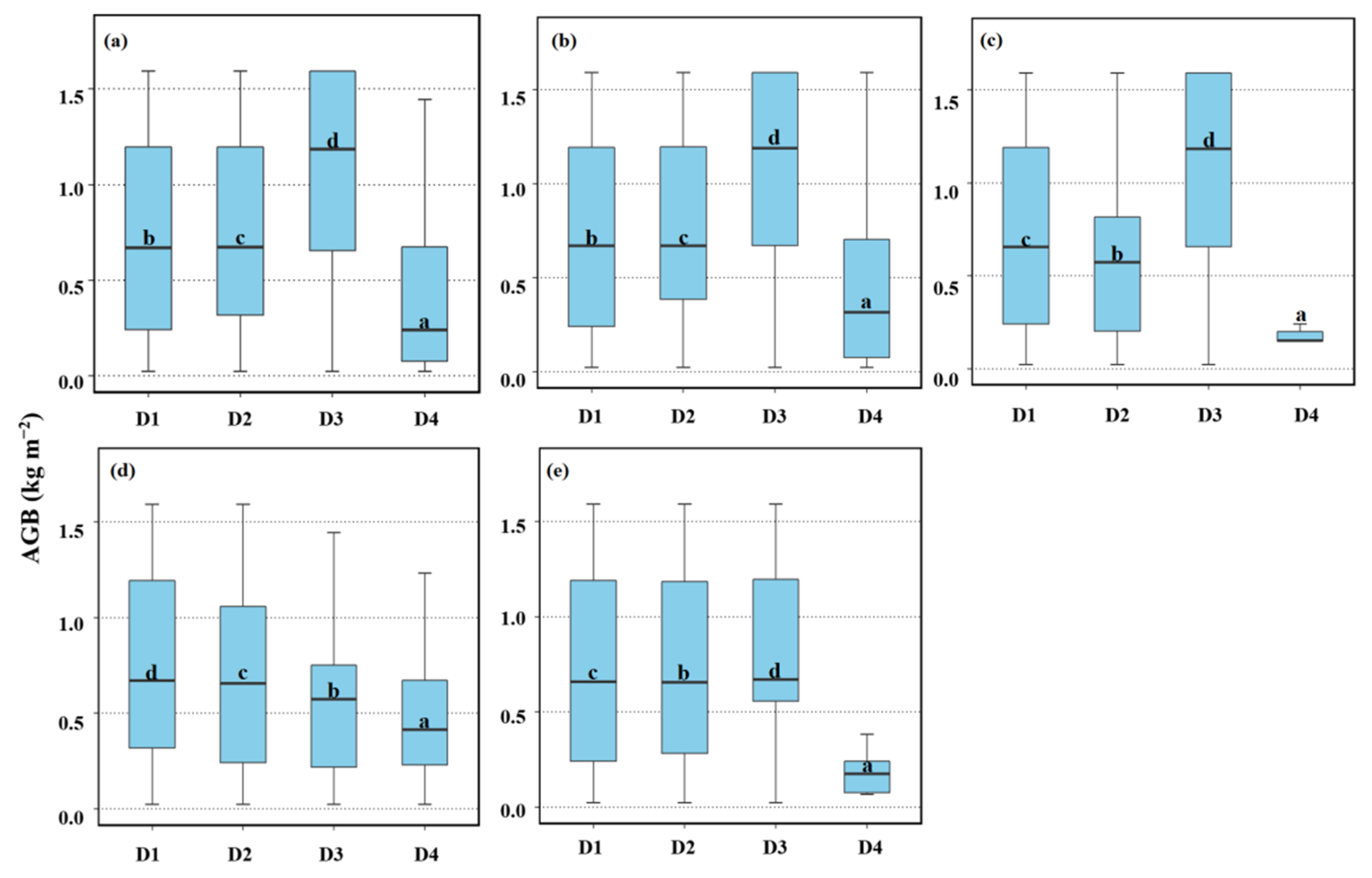
3.3. Impacts of Tidal Creeks on the AGB of Different Salt Marsh Communities

For the overall AGB, as the distance from the tidal creek increased, the AGB of all salt marsh vegetation overall increased from 0.73 kg m−2 in D1 to 1.01 kg m−2 in D3 and decreased from D3 to D4 (0.47 kg m−2), and there were significant (p < 0.05) differences in AGB at different distance gradients (Figure 5a). For different vegetation communities, the AGB of PA showed similar trends (Figure 5b). The average AGB of PA increased from 0.75 kg m−2 in D1 to 1.04 kg m−2 in D3 and dropped from 1.04 kg m−2 in D3 to 0.49 kg m−2 in D4. The mean AGB of CS was decreased from 0.76 kg m−2 in D1 to 0.49 kg m−2 in D4, with significant (p < 0.05) differences in AGB at different distance gradients (Figure 5d). The mean AGB of IC and SM, respectively, showed a general decline from 0.70 kg m−2 in D1 to 0.18 kg m−2 in D4 (Figure 5c) and from 0.70 kg m−2 in D1 to 0.22 kg m−2 in D4 (Figure 5e), with significant (p < 0.05) differences in AGB at different distance gradients.

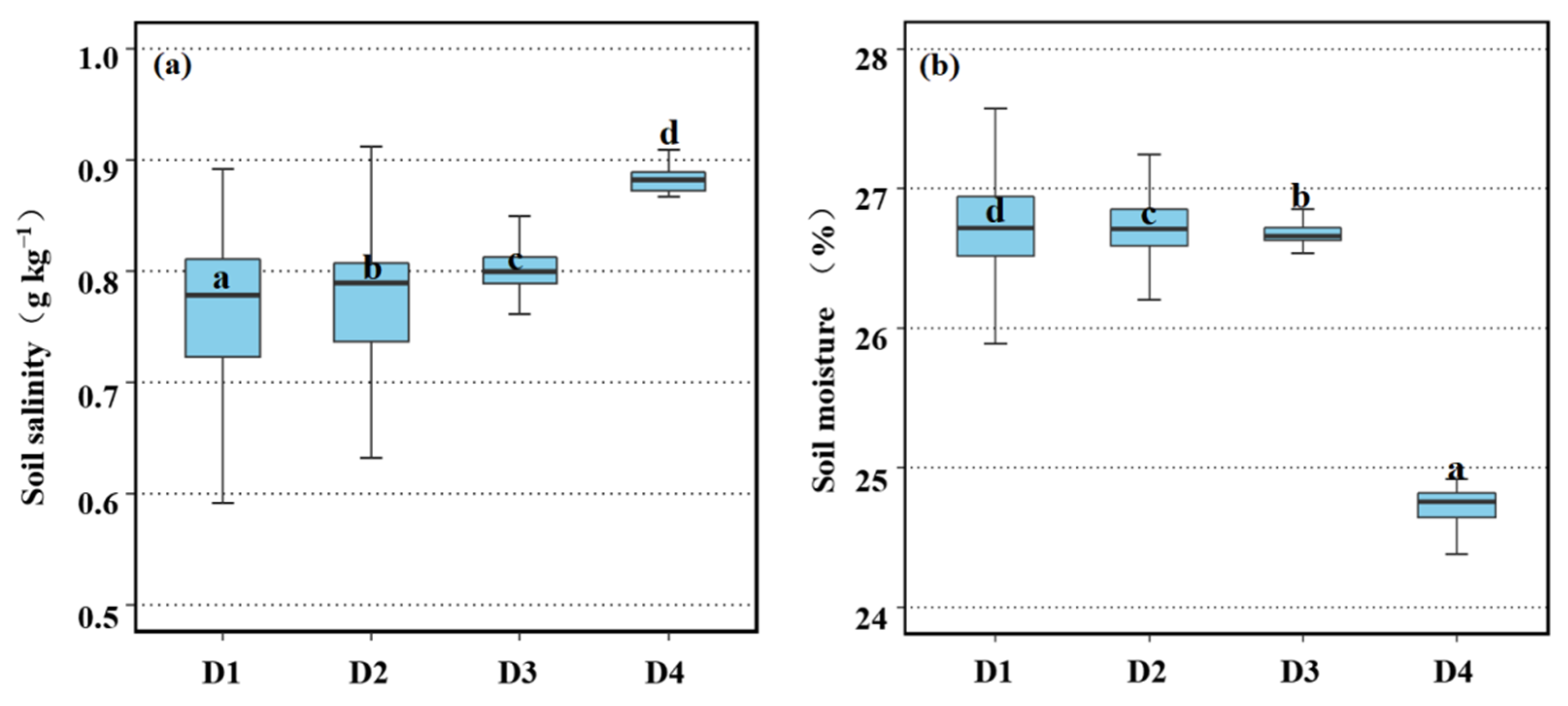
3.4. Spatial Variation in Soil Salinity and Moisture

Soil salinity and moisture changed significantly with increasing distance from the tidal creeks in our study area. Compared with soil salinity between different distance gradients, we found that the mean soil salinity of salt marsh increased from 0.75 g kg−1 in D1 to 0.87 g kg−1 in D4, and there were significant (p < 0.05) differences in soil salinity at different distance gradients (Figure 6a). The mean soil moisture content decreased from 26.75% in D1 to 24.82% in D4, with significant (p < 0.05) differences in soil moisture at different distance gradients (Figure 6b).

4. Discussion

4.1. Impacts of Tidal Creeks on the Spatial Distribution of Salt Marsh Communities and Their AGB

Our study shows that the spatial patterns of different salt marsh communities were inconsistently affected by distance from tidal creeks. The percentage of area compositions of SM, CS, and IC was decreased, respectively, and the communities of SM, CS, and IC were more likely to be distributed near tidal creeks. The PA community was mainly distributed far away from the tidal creeks, and its percentage of area compositions increased. The result fits with existing research, which shows that there is a positive relation between the density of PA communities and their vertical distance from tidal creeks [57]. We found that soil salinity increases with increasing distance from tidal creeks. The salinity of soil increased with distance from tidal creeks increasing [58], which restricted the growth of SM, IC, and CS [59,60]. Thus, it means that the distance from the tidal creeks affects the spatial distribution of salt marsh vegetation by increasing salinity stress. Previous research has shown that the reasons for salt marsh plant zoning are both abiotic, partly related to the variability of soil and tidal conditions [16], and biological, caused by resource competition among species and biological response to periodic interference [61]. Moreover, the distribution of the CS community is sparse at all distance gradients. This is likely to be dictated by its competitive inferiority to the IC community [62].
The total salt marsh AGB increased as distances from tidal creeks increased. This may also be shaped by the gradients of environmental factors, particularly soil moisture, at different distances from tidal creeks. For example, a previous study found a significant decline in plant productivity of salt marsh in response to flooding [63], and that the frequency of tidal flooding and the duration of tidal flooding increased with distances from tidal creeks decreasing [64,65]. In our study, we also found a decline in soil moisture with increasing distance from tidal creeks in the study area. The tidal creeks form a significant gradient of soil moisture, which varies along the distance of tidal creeks. Therefore, the distance from the tidal creek has a deep impact on community succession of salt marshes by controlling tidal flooding. Considering the varying AGB of different salt marsh species (Figure 4d), the spatial pattern of the AGB of salt marshes was different. Therefore, our results demonstrate that tidal creeks are the key factors affecting the spatial distribution of vegetation communities and their AGB in coastal salt marshes.
Our results show that the spatial variability of soil moisture and salinity at distance gradients from the tidal creeks causes the spatial distributions of plant vegetation and its AGB at different distances from tidal creeks. However, the previous analysis shows that simple correlations between plant zoning and distance from the nearest creek are not generally effective and cannot be spread to different regions, even if tidal conditions are the same [66]. The spatial morphology and distribution characteristics of tidal creeks influence the spatial distribution and AGB of coastal wetlands [26]. The topography of sediment creeks affects the distribution of salt marsh vegetation and thus its AGB [67]. In addition, the feedback between plant growth and the geomorphological developments of the depositional environment leads to elevated substrate topography [68]. In future research, we will focus on the relationships between the AGB of salt marsh vegetation and the morphological characteristics or the topography of tidal creeks to explore the mechanism affecting the spatial distribution of AGB of salt marsh vegetation.

4.2. Advantages of AGB Estimation Using UAV-LiDAR Data and Machine Learning Approaches

UAV-LiDAR data were successfully applied to estimate the AGB of coastal salt marsh communities. We constructed height variables, including the average height (H), the derived factors H2 and logH within a 1 m2 square based on UAV-LiDAR point cloud data for AGB estimation of salt marsh vegetation. A good model fit (R2 = 0.90, RMSE = 0.09 kg m−2) using the model developed within our study. The results show that UAV-LiDAR data have a high potential for estimating the AGB of coastal salt marsh communities, which is similar to the application of LiDAR data in AGB estimation in terrestrial ecosystems [69]. The AGB map provides interesting insights for salt marsh vegetation’s growth dynamics of salt marsh vegetation related to canopy height. The UAV-LiDAR data have more advantages in seizing the subtle resolution, plant three-dimensional structure, and digital terrain with a lower cost and higher mobility [70,71]. Nonetheless, since UAV-acquired datasets can provide more information on objects [72], more plant structure parameters can be included in the estimation model, which may further improve the estimation accuracy of salt marsh AGB. This will solve the difficulty, to some extent, in estimating the carbon storage in the AGB in salt marsh on the regional scale and greatly promote studies relating to the structure, function, and carbon cycle dynamics of wetland ecosystems in estuarine and coastal zones.
Moreover, the machine learning approaches, particularly the random forest algorithm, demonstrated a strong suitability to construct a salt marsh AGB prediction model in this study, which has also been confirmed in other ecosystems, such as crop [73] and forest [74]. Compared with several regression analysis methods, the random forest algorithm has certain advantages and a high consistency (R2 = 0.89, RMSE = 13 kg m−2) between fitted AGB and observed AGB throughout the study area. This means that a general AGB estimation model for mixed salt marsh species based on a random forest algorithm has higher applicability in estimating salt marsh aboveground C storage for complex communities.
Our study shows that a coupling machine learning algorithm and UAV-LiDAR data provide a practical approach for estimating AGB in salt marsh wetlands, which is worthy of widespread application in other regions in the future. In particular, combining UAV-LiDAR data with other RS data can significantly promote the accuracy of short-term vegetation parameter estimation [75]. In future research, we will attempt to improve the estimation accuracy of salt marsh AGB by fusing other RS data with UAV-LiDAR data.

4.3. Management of Coastal Salt Marsh

In our study area, coastal salt marshes are the major component in the C cycle in the Yangtze River Estuary [76], and tidal creeks play an important role in shaping the spatial patterns of salt marsh vegetation and C storage [77]. Thus, it is of great importance to maintain the productivity of the salt marsh wetland ecosystem [78]. Moreover, our study accurately estimated large-scale patterns of salt marsh AGB to reflect the spatial distribution of aboveground C storage. In addition, quantifying the impacts of the distance from tidal creeks on the spatial distribution of salt marsh communities and their AGB is critical to ensure reasonable local planning, biodiversity protection, and sustainable development of wetland resources.

5. Conclusions

Based on high-resolution images and LiDAR data collected using UAV platforms, the spatial distribution of select salt marsh communities and the AGB were estimated. Here, we demonstrate that the distance from tidal creeks has a significant influence on the communities’ spatial patterns and the AGB of salt marsh vegetation by altering soil salinity and soil moisture conditions. Our results confirm that the UAV-LiDAR data coupled random forest algorithm is a possible convenient and effective means to detect AGB of salt marshes. In conclusion, our study shows an effective approach to estimating the aboveground C storage of salt marshes, highlighting how its accurate estimation plays a vital role in making reasonable scientific measures to manage and protect coastal ecosystems.

Author Contributions

Designed the research, Y.-N.T. and J.M.; collected the data, Y.-N.T., J.-X.X., Y.-C.W. and H.-Q.G.; analyzed the data, Y.-N.T. and Y.-C.W.; wrote the paper, Y.-N.T.; reviewed the draft, J.M. and W.-B.W. All authors have read and agreed to the published version of the manuscript.

Funding

This research was funded by the Natural Science Foundation of China, grant number U2106209, and the Scientific Research Program of Shanghai Science and Technology Commission, grant number 21ZR1405600 and 20dz1204702.

Data Availability Statement

Not applicable. The LiDAR data of this study are available on request from the corresponding author.

Acknowledgments

We thank Tao-Yan Shen, Yi-Fei Liu, and Shu-Yun Wei for their field investigation.

Conflicts of Interest

The authors declare that they have no conflict of interest.

References

  1. Edge, R.S.; Sullivan, M.J.; Pedley, S.M.; Mossman, H.L. Species interactions modulate the response of saltmarsh plants to flooding. Ann. Bot. 2020, 125, 315–324. [Google Scholar] [CrossRef] [PubMed]
  2. Pellegrini, E.; Boscutti, F.; De Nobili, M.; Casolo, V. Plant traits shape the effects of tidal flooding on soil and plant communities in saltmarshes. Plant Ecol. 2018, 219, 823–835. [Google Scholar] [CrossRef]
  3. Kelleway, J.J.; Cavanaugh, K.; Rogers, K.; Feller, I.C.; Ens, E.; Doughty, C.; Saintilan, N. Review of the ecosystem service implications of mangrove encroachment into salt marshes. Glob. Change Biol. 2017, 23, 3967–3983. [Google Scholar] [CrossRef] [PubMed]
  4. Mitsch, W.J.; Bernal, B.; Hernandez, M.E. Ecosystem services of wetlands. Int. J. Biodivers. Sci. Ecosyst. Serv. Manag. 2015, 11, 1–4. [Google Scholar] [CrossRef] [Green Version]
  5. Beaumont, N.J.; Jones, L.; Garbutt, A.; Hansom, J.; Toberman, M. The value of carbon sequestration and storage in coastal habitats. Estuar. Coast. Shelf Sci. 2014, 137, 32–40. [Google Scholar] [CrossRef] [Green Version]
  6. Pendleton, L.; Donato, D.C.; Murray, B.C.; Crooks, S.; Jenkins, W.A.; Sifleet, S.; Craft, C.; Fourqurean, J.W.; Kauffman, J.B.; Marbà, N. Estimating global “blue carbon” emissions from conversion and degradation of vegetated coastal ecosystems. PLoS ONE 2012, 7, e43542. [Google Scholar] [CrossRef] [Green Version]
  7. Duarte, C.M.; Middelburg, J.J.; Caraco, N. Major role of marine vegetation on the oceanic carbon cycle. Biogeosciences 2005, 2, 1–8. [Google Scholar] [CrossRef] [Green Version]
  8. Mcleod, E.; Chmura, G.L.; Bouillon, S.; Salm, R.; Björk, M.; Duarte, C.M.; Lovelock, C.E.; Schlesinger, W.H.; Silliman, B.R. A blueprint for blue carbon: Toward an improved understanding of the role of vegetated coastal habitats in sequestering CO2. Front. Ecol. Environ. 2011, 9, 552–560. [Google Scholar] [CrossRef] [Green Version]
  9. Adam, E.; Mutanga, O.; Rugege, D. Multispectral and hyperspectral remote sensing for identification and mapping of wetland vegetation: A review. Wetl. Ecol. Manag. 2010, 18, 281–296. [Google Scholar] [CrossRef]
  10. Chen, J.; Gu, S.; Shen, M.; Tang, Y.; Matsushita, B. Estimating aboveground biomass of grassland having a high canopy cover: An exploratory analysis of in situ hyperspectral data. Int. J. Remote Sens. 2009, 30, 6497–6517. [Google Scholar] [CrossRef]
  11. Du, Y.; Wang, J.; Liu, Z.; Yu, H.; Li, Z.; Cheng, H. Evaluation on spaceborne multispectral images, airborne hyperspectral, and LiDAR data for extracting spatial distribution and estimating aboveground biomass of wetland vegetation suaeda salsa. IEEE J. Sel. Top. Appl. Earth Obs. Remote Sens. 2018, 12, 200–209. [Google Scholar] [CrossRef]
  12. Wang, J.; Liu, Z.; Yu, H.; Li, F. Mapping Spartina alterniflora biomass using LiDAR and hyperspectral data. Remote Sens. 2017, 9, 589. [Google Scholar] [CrossRef] [Green Version]
  13. Bertness, M.D.; Pennings, S.C. Spatial Variation in Process and Pattern in Salt Marsh Plant Communities in Eastern North America. In Concepts and Controversies in Tidal Marsh Ecology; Springer: New, York, NY, USA, 2002; pp. 39–57. [Google Scholar]
  14. Crain, C.M.; Silliman, B.R.; Bertness, S.L.; Bertness, M.D. Physical and biotic drivers of plant distribution across estuarine salinity gradients. Ecology 2004, 85, 2539–2549. [Google Scholar] [CrossRef] [Green Version]
  15. Xue, L.; Jiang, J.; Li, X.; Yan, Z.; Zhang, Q.; Ge, Z.; Tian, B.; Craft, C. Salinity Affects Topsoil Organic Carbon Concentrations Through Regulating Vegetation Structure and Productivity. J. Geophys. Res. Biogeosciences 2020, 125, e2019JG005217. [Google Scholar] [CrossRef]
  16. Pennings, S.C.; Grant, M.-B.; Bertness, M.D. Plant zonation in low-latitude salt marshes: Disentangling the roles of flooding, salinity and competition. J. Ecol. 2005, 93, 159–167. [Google Scholar] [CrossRef]
  17. Kearney, W.S.; Fagherazzi, S. Salt marsh vegetation promotes efficient tidal channel networks. Nat. Commun. 2016, 7, 12287. [Google Scholar] [CrossRef] [Green Version]
  18. Wang, X.; Li, Y.; Meng, H.; Dong, H.; Guo, Y.; Tong, S. Distribution pattern of plant community in new-born coastal wetland in the Yellow River Delta. Sci. Geogr. Sin. 2015, 35, 1021–1026. [Google Scholar]
  19. Zhao, X.; Cui, B.; Sun, T.; He, Q. The relationship between the spatial distribution of vegetation and soil environmental factors in the tidal creek areas of the Yellow River Delta. Ecol. Environ. Sci. 2010, 19, 1855–1861. [Google Scholar]
  20. Balling, S.S.; Resh, V.H. The influence of mosquito control recirculation ditches on plant biomass, production and composition in two San Francisco Bay salt marshes. Estuar. Coast. Shelf Sci. 1983, 16, 151–161. [Google Scholar] [CrossRef]
  21. Byrd, K.B.; O’Connell, J.L.; Di Tommaso, S.; Kelly, M. Evaluation of sensor types and environmental controls on mapping biomass of coastal marsh emergent vegetation. Remote Sens. Environ. 2014, 149, 166–180. [Google Scholar] [CrossRef]
  22. Ozesmi, S.L.; Bauer, M.E. Satellite remote sensing of wetlands. Wetl. Ecol. Manag. 2002, 10, 381–402. [Google Scholar] [CrossRef]
  23. Miller, G.J.; Morris, J.T.; Wang, C. Estimating aboveground biomass and its spatial distribution in coastal wetlands utilizing planet multispectral imagery. Remote Sens. 2019, 11, 2020. [Google Scholar] [CrossRef] [Green Version]
  24. Lumbierres, M.; Méndez, P.F.; Bustamante, J.; Soriguer, R.; Santamaría, L. Modeling biomass production in seasonal wetlands using MODIS NDVI land surface phenology. Remote Sens. 2017, 9, 392. [Google Scholar] [CrossRef] [Green Version]
  25. Vaghela, B.; Chirakkal, S.; Putrevu, D.; Solanki, H. Modelling above ground biomass of Indian mangrove forest using dual-pol SAR data. Remote Sens. Appl. Soc. Environ. 2021, 21, 100457. [Google Scholar] [CrossRef]
  26. Tian, Y.; Zhang, Q.; Huang, H.; Huang, Y.; Tao, J.; Zhou, G.; Zhang, Y.; Yang, Y.; Lin, J. Aboveground biomass of typical invasive mangroves and its distribution patterns using UAV-LiDAR data in a subtropical estuary: Maoling River estuary, Guangxi, China. Ecol. Indic. 2022, 136, 108694. [Google Scholar] [CrossRef]
  27. Fatoyinbo, T.; Feliciano, E.A.; Lagomasino, D.; Lee, S.K.; Trettin, C. Estimating mangrove aboveground biomass from airborne LiDAR data: A case study from the Zambezi River delta. Environ. Res. Lett. 2018, 13, 025012. [Google Scholar] [CrossRef] [Green Version]
  28. Guo, M.; Li, J.; Sheng, C.; Xu, J.; Wu, L. A review of wetland remote sensing. Sensors 2017, 17, 777. [Google Scholar] [CrossRef] [PubMed] [Green Version]
  29. Dalponte, M.; Coops, N.C.; Bruzzone, L.; Gianelle, D. Analysis on the use of multiple returns LiDAR data for the estimation of tree stems volume. IEEE J. Sel. Top. Appl. Earth Obs. Remote Sens. 2009, 2, 310–318. [Google Scholar] [CrossRef]
  30. Hsu, A.J.; Kumagai, J.; Favoretto, F.; Dorian, J.; Guerrero Martinez, B.; Aburto-Oropeza, O. Driven by Drones: Improving Mangrove Extent Maps Using High-Resolution Remote Sensing. Remote Sens. 2020, 12, 3986. [Google Scholar] [CrossRef]
  31. Cohen, M.C.; de Souza, A.V.; Liu, K.-b.; Rodrigues, E.; Yao, Q.; Ryu, J.; Dietz, M.; Pessenda, L.C.; Rossetti, D. Effects of the 2017–2018 winter freeze on the northern limit of the American mangroves, Mississippi River delta plain. Geomorphology 2021, 394, 107968. [Google Scholar] [CrossRef]
  32. Laporte-Fauret, Q.; Marieu, V.; Castelle, B.; Michalet, R.; Bujan, S.; Rosebery, D. Low-cost UAV for high-resolution and large-scale coastal dune change monitoring using photogrammetry. J. Mar. Sci. Eng. 2019, 7, 63. [Google Scholar] [CrossRef] [Green Version]
  33. Fabbri, S.; Grottoli, E.; Armaroli, C.; Ciavola, P. Using High-Spatial Resolution UAV-Derived Data to Evaluate Vegetation and Geomorphological Changes on a Dune Field Involved in a Restoration Endeavour. Remote Sens. 2021, 13, 1987. [Google Scholar] [CrossRef]
  34. Rende, S.F.; Bosman, A.; Di Mento, R.; Bruno, F.; Lagudi, A.; Irving, A.D.; Dattola, L.; Giambattista, L.D.; Lanera, P.; Proietti, R. Ultra-high-resolution mapping of Posidonia oceanica (L.) delile meadows through acoustic, optical data and object-based image classification. J. Mar. Sci. Eng. 2020, 8, 647. [Google Scholar] [CrossRef]
  35. Klemas, V.V. Coastal and environmental remote sensing from unmanned aerial vehicles: An overview. J. Coast. Res. 2015, 31, 1260–1267. [Google Scholar] [CrossRef] [Green Version]
  36. Whitehead, K.; Hugenholtz, C.H. Remote sensing of the environment with small unmanned aircraft systems (UASs), part 1: A review of progress and challenges. J. Unmanned Veh. Syst. 2014, 2, 69–85. [Google Scholar] [CrossRef]
  37. Xu, Z.; Li, W.; Li, Y.; Shen, X.; Ruan, H. Estimation of secondary forest parameters by integrating image and point cloud-based metrics acquired from unmanned aerial vehicle. J. Appl. Remote Sens. 2019, 14, 022204. [Google Scholar] [CrossRef] [Green Version]
  38. Kalacska, M.; Chmura, G.; Lucanus, O.; Bérubé, D.; Arroyo-Mora, J. Structure from motion will revolutionize analyses of tidal wetland landscapes. Remote Sens. Environ. 2017, 199, 14–24. [Google Scholar] [CrossRef]
  39. Doughty, C.L.; Cavanaugh, K.C. Mapping coastal wetland biomass from high resolution unmanned aerial vehicle (UAV) imagery. Remote Sens. 2019, 11, 540. [Google Scholar] [CrossRef] [Green Version]
  40. Zhang, X.; Xiao, X.; Wang, X.; Xu, X.; Chen, B.; Wang, J.; Ma, J.; Zhao, B.; Li, B. Quantifying expansion and removal of Spartina alterniflora on Chongming island, China, using time series Landsat images during 1995–2018. Remote Sens. Environ. 2020, 247, 111916. [Google Scholar] [CrossRef]
  41. Jiang, Y.; Du, J.; Zhang, J.; Zhang, W.; Zhang, J. The determination of sedimentation rates in various vegetational zones of Chongming tidal flat of the Changjiang Estuary. Acta Oceanol. Sin. 2012, 34, 114–121. [Google Scholar]
  42. Shilun, Y. A study of coastal morphodynamics on the muddy islands in the Changjiang River estuary. J. Coast. Res. 1999, 15, 32–44. [Google Scholar]
  43. Ding, W.-H.; Jiang, J.-Y.; Li, X.-Z.; Huang, X.; Li, X.-Z.; Zhou, Y.-X.; Tang, C.-D. Spatial distribution of species and influencing factors across salt marsh in southern Chongming Dongtan. Chin. J. Plant. Ecol. 2015, 39, 704–716. [Google Scholar]
  44. Gao, Z.; Zhang, L. Multi-seasonal spectral characteristics analysis of coastal salt marsh vegetation in Shanghai, China. Estuar. Coast. Shelf Sci. 2006, 69, 217–224. [Google Scholar] [CrossRef]
  45. Yan, Q.; Lu, J.; He, W. Succession character of salt marsh vegetations in Chongming Dongtan wetland. J. Appl. Ecol. 2007, 18, 1097–1101. [Google Scholar]
  46. Foody, G.M. Status of land cover classification accuracy assessment. Remote Sens. Environ. 2002, 80, 185–201. [Google Scholar] [CrossRef]
  47. Uebersax, J.S. Diversity of decision-making models and the measurement of interrater agreement. Psychol. Bull. 1987, 101, 140. [Google Scholar] [CrossRef]
  48. Tung, F.; LeDrew, E. The determination of optimal threshold levels for change detection using various accuracy indexes. Photogramm. Eng. Remote Sens. 1988, 54, 1449–1454. [Google Scholar]
  49. Story, M.; Congalton, R.G. Accuracy assessment: A user’s perspective. Photogramm. Eng. Remote Sens. 1986, 52, 397–399. [Google Scholar]
  50. Tranmer, M.; Elliot, M. Multiple linear regression. Cathie Marsh Cent. Census Surv. Res. (CCSR) 2008, 5, 1–5. [Google Scholar]
  51. Guisan, A.; Edwards, T.C., Jr.; Hastie, T. Generalized linear and generalized additive models in studies of species distributions: Setting the scene. Ecol. Model. 2002, 157, 89–100. [Google Scholar] [CrossRef] [Green Version]
  52. Elith, J.; Leathwick, J.R.; Hastie, T. A working guide to boosted regression trees. J. Anim. Ecol. 2008, 77, 802–813. [Google Scholar] [CrossRef] [PubMed]
  53. Zhang, Z. Artificial Neural Network. In Multivariate Time Series Analysis in Climate and Environmental Research; Springer: New, York, NY, USA, 2018; pp. 1–35. [Google Scholar]
  54. Engel, Y.; Mannor, S.; Meir, R. The kernel recursive least-squares algorithm. IEEE Trans. Signal Process. 2004, 52, 2275–2285. [Google Scholar] [CrossRef]
  55. Breiman, L. Random forests. Mach. Learn. 2001, 45, 5–32. [Google Scholar] [CrossRef] [Green Version]
  56. Shen, W.; Li, M.; Huang, C.; Tao, X.; Wei, A. Annual Forest aboveground biomass changes mapped using ICESat/GLAS measurements, historical inventory data, and time-series optical and radar imagery for Guangdong province, China. Agric. For. Meteorol. 2018, 259, 23–38. [Google Scholar] [CrossRef] [Green Version]
  57. Wu, Y.; Liu, J.; Yan, G.; Zhai, J.; Cong, L.; Dai, L.; Zhang, Z.; Zhang, M. The size and distribution of tidal creeks affects salt marsh restoration. J. Environ. Manag. 2020, 259, 110070. [Google Scholar] [CrossRef]
  58. Snow, A.A.; Vince, S.W. Plant zonation in an Alaskan salt marsh: II. An experimental study of the role of edaphic conditions. J. Ecol. 1984, 7, 669–684. [Google Scholar] [CrossRef]
  59. He, Y.; Li, X.; Ma, Z.; Sun, Y.; Jia, Y. Vegetation zonation related to the edaphic factors in the East headland of Chongming Island. Acta Ecol. Sin. 2010, 30, 4919–4927. [Google Scholar]
  60. Li, W.-Q.; Xiao-Jing, L.; Khan, M.A.; Gul, B. Relationship between soil characteristics and halophytic vegetation in coastal region of North China. Pak. J. Bot. 2008, 40, 1081–1090. [Google Scholar]
  61. Emery, N.C.; Ewanchuk, P.J.; Bertness, M.D. Competition and salt-marsh plant zonation: Stress tolerators may be dominant competitors. Ecology 2001, 82, 2471–2485. [Google Scholar] [CrossRef]
  62. Ishikawa, S.-I.; Kachi, N. Shoot population dynamics of Carex kobomugi on a coastal sand dune in relation to its zonal distribution. Aust. J. Bot. 1998, 46, 111–121. [Google Scholar] [CrossRef]
  63. Janousek, C.N.; Mayo, C. Plant responses to increased inundation and salt exposure: Interactive effects on tidal marsh productivity. Plant Ecol. 2013, 214, 917–928. [Google Scholar] [CrossRef]
  64. Brown, A.M.; Bledsoe, C. Spatial and temporal dynamics of mycorrhizas in Jaumea carnosa, a tidal saltmarsh halophyte. J. Ecol. 1996, 84, 703–715. [Google Scholar] [CrossRef]
  65. Valiela, I.; Teal, J.M.; Deuser, W.G. The nature of growth forms in the salt marsh grass Spartina alterniflora. Am. Nat. 1978, 112, 461–470. [Google Scholar] [CrossRef]
  66. Bockelmann, A.-C.; Bakker, J.P.; Neuhaus, R.; Lage, J. The relation between vegetation zonation, elevation and inundation frequency in a Wadden Sea salt marsh. Aquat. Bot. 2002, 73, 211–221. [Google Scholar] [CrossRef]
  67. Mossman, H.L.; Grant, A.; Davy, A.J. Manipulating saltmarsh microtopography modulates the effects of elevation on sediment redox potential and halophyte distribution. J. Ecol. 2020, 108, 94–106. [Google Scholar] [CrossRef]
  68. Cao, H.; Zhu, Z.; van Belzen, J.; Gourgue, O.; van de Koppel, J.; Temmerman, O.S.; Herman, P.M.; Zhang, L.; Yuan, L.; Bouma, T.J. Salt marsh establishment in poorly consolidated muddy systems: Effects of surface drainage, elevation, and plant age. Ecosphere 2021, 12, e03755. [Google Scholar] [CrossRef]
  69. Wang, D.; Wan, B.; Liu, J.; Su, Y.; Guo, Q.; Qiu, P.; Wu, X. Estimating aboveground biomass of the mangrove forests on northeast Hainan Island in China using an upscaling method from field plots, UAV-LiDAR data and Sentinel-2 imagery. Int. J. Appl. Earth Obs. Geoinf. 2020, 85, 101986. [Google Scholar] [CrossRef]
  70. Janowski, L.; Tylmann, K.; Trzcinska, K.; Rudowski, S.; Tegowski, J. Exploration of glacial landforms by object-based image analysis and spectral parameters of digital elevation model. IEEE Trans. Geosci. Remote Sens. 2021, 60, 1–17. [Google Scholar] [CrossRef]
  71. Guo, Q.; Su, Y.; Hu, T.; Zhao, X.; Wu, F.; Li, Y.; Liu, J.; Chen, L.; Xu, G.; Lin, G. An integrated UAV-borne lidar system for 3D habitat mapping in three forest ecosystems across China. Int. J. Remote Sens. 2017, 38, 2954–2972. [Google Scholar] [CrossRef]
  72. Maimaitijiang, M.; Sagan, V.; Sidike, P.; Hartling, S.; Esposito, F.; Fritschi, F.B. Soybean yield prediction from UAV using multimodal data fusion and deep learning. Remote Sens. Environ. 2020, 237, 111599. [Google Scholar] [CrossRef]
  73. Xu, J.-X.; Ma, J.; Tang, Y.-N.; Wu, W.-X.; Shao, J.-H.; Wu, W.-B.; Wei, S.-Y.; Liu, Y.-F.; Wang, Y.-C.; Guo, H.-Q. Estimation of Sugarcane Yield Using a Machine Learning Approach Based on UAV-LiDAR Data. Remote Sens. 2020, 12, 2823. [Google Scholar] [CrossRef]
  74. Gleason, C.J.; Im, J. Forest biomass estimation from airborne LiDAR data using machine learning approaches. Remote Sens. Environ. 2012, 125, 80–91. [Google Scholar] [CrossRef]
  75. Zhu, Y.; Zhao, C.; Yang, H.; Yang, G.; Han, L.; Li, Z.; Feng, H.; Xu, B.; Wu, J.; Lei, L. Estimation of maize above-ground biomass based on stem-leaf separation strategy integrated with LiDAR and optical remote sensing data. PeerJ 2019, 7, e7593. [Google Scholar] [CrossRef] [PubMed] [Green Version]
  76. Yuan, Y.; Li, X.; Jiang, J.; Xue, L.; Craft, C.B. Distribution of organic carbon storage in different salt-marsh plant communities: A case study at the Yangtze estuary. Estuar. Coast. Shelf Sci. 2020, 243, 106900. [Google Scholar] [CrossRef]
  77. Sanderson, E.W.; Foin, T.C.; Ustin, S.L. A simple empirical model of salt marsh plant spatial distributions with respect to a tidal channel network. Ecol. Model. 2001, 139, 293–307. [Google Scholar] [CrossRef]
  78. Call, M.; Sanders, C.J.; Macklin, P.A.; Santos, I.R.; Maher, D.T. Carbon outwelling and emissions from two contrasting mangrove creeks during the monsoon storm season in Palau, Micronesia. Estuar. Coast. Shelf Sci. 2019, 218, 340–348. [Google Scholar] [CrossRef]
Figure 1. The location of the research area and sampling sites. (a) The site on Chongming Island, Shanghai, in China. (b) The study area of Dongtan on Chongming Island. (c) The sampling area on Dongtan.
Remotesensing 14 01839 g001
Figure 2. The spatial distribution and area compositions of salt marsh communities. (a) Map of coastal salt marsh vegetation classification. (b) The percentage of salt marsh plant at different distance gradients from tidal creeks. PA: Phragmites australis; IC: Imperata cylindrica; CS: Carex scabrifolia; SM: Scirpus mariqueter. D1: 0–100 m; D2: 100–200 m; D3: 200–300 m; D4: 300–400 m; D5: higher than 400 m.
Remotesensing 14 01839 g002
Figure 3. The relationship between measured and predicted AGB of coastal salt marsh vegetation. (a) MLR; (b) KRLS; (c) ANN; (d) GBM; (e) RFR; (f) GLM. The red full line indicates a linear fit, and the blue line of dashes indicates a 1:1 line.
Remotesensing 14 01839 g003
Figure 4. The spatial distribution, validation, and comparisons of AGB for different salt marsh communities. (a) Mapping the AGB of salt marsh vegetation using UAV-LiDAR data and a random forest model. (b) The mean AGB for different salt marsh communities. (c) Regression fitting between AGB in the field survey and AGB predicted based on UAV-LiDAR data and a random forest model. The red full line indicates a linear fit, and the blue line of dashes indicates a 1:1 line. PA: Phragmites australis; CS: Carex scabrifolia; IC: Imperata cylindrica; SM: Scirpus mariqueter. (d) Density distribution curve of the predicted AGB. The data with different lowercase letters show a significant difference.
Remotesensing 14 01839 g004
Figure 5. Comparisons of salt marsh AGB of different distances from tidal creeks. (a) represents the AGB change trend of the whole vegetation community; (be) represent the AGB change trend of PA, IC, CS, and SM, respectively. The data with different lowercase letters show a significant difference. D1: 0–50 m; D2: 50–100 m; D3: 100–150 m; D4: 150–200 m.
Remotesensing 14 01839 g005
Figure 6. Comparisons of soil salinity and moisture at different distances from tidal creeks. (a) Comparisons of soil salinity at different distances from tidal creeks. (b) Comparisons of soil moisture at different distances from tidal creeks. The data with different lower-case letters show a significant difference. D1: 0–50 m; D2: 50–100 m; D3: 100–150 m; D4: 150–200 m.
Remotesensing 14 01839 g006
Table 1. A summary of field vegetation sampling points.
ClassVegetation CommunitySpecies CompositionNumber of SamplesAverage Value of an AGB (kg m−2)
PAPhragmites australisPhragmites australis, Carex scabrifolia, Imperata cylindrica210.56
ICImperata cylindricaImperata cylindrica, Phragmites australis90.21
SMScirpus mariqueterScirpus mariqueter90.29
CSCarex scabrifoliaCarex scabrifolia, Phragmites australis210.21
Table 2. A summary of the accuracy assessment for salt marsh communities (PA: Phragmites australis; CS: Carex scabrifolia; IC: Imperata cylindrica; SM: Scirpus mariqueter).
Community TypeProducer Accuracy (%)User Accuracy (%)
PA97.0796.89
IC79.1798.88
SM99.8895.15
CS96.4698.93
Publisher’s Note: MDPI stays neutral with regard to jurisdictional claims in published maps and institutional affiliations.

