
Optical Turbulence Profile in Marine Environment with Artificial Neural Network Model

 ,
,
Abstract
:1. Introduction
2. Methodology
2.1. GA-BP Model
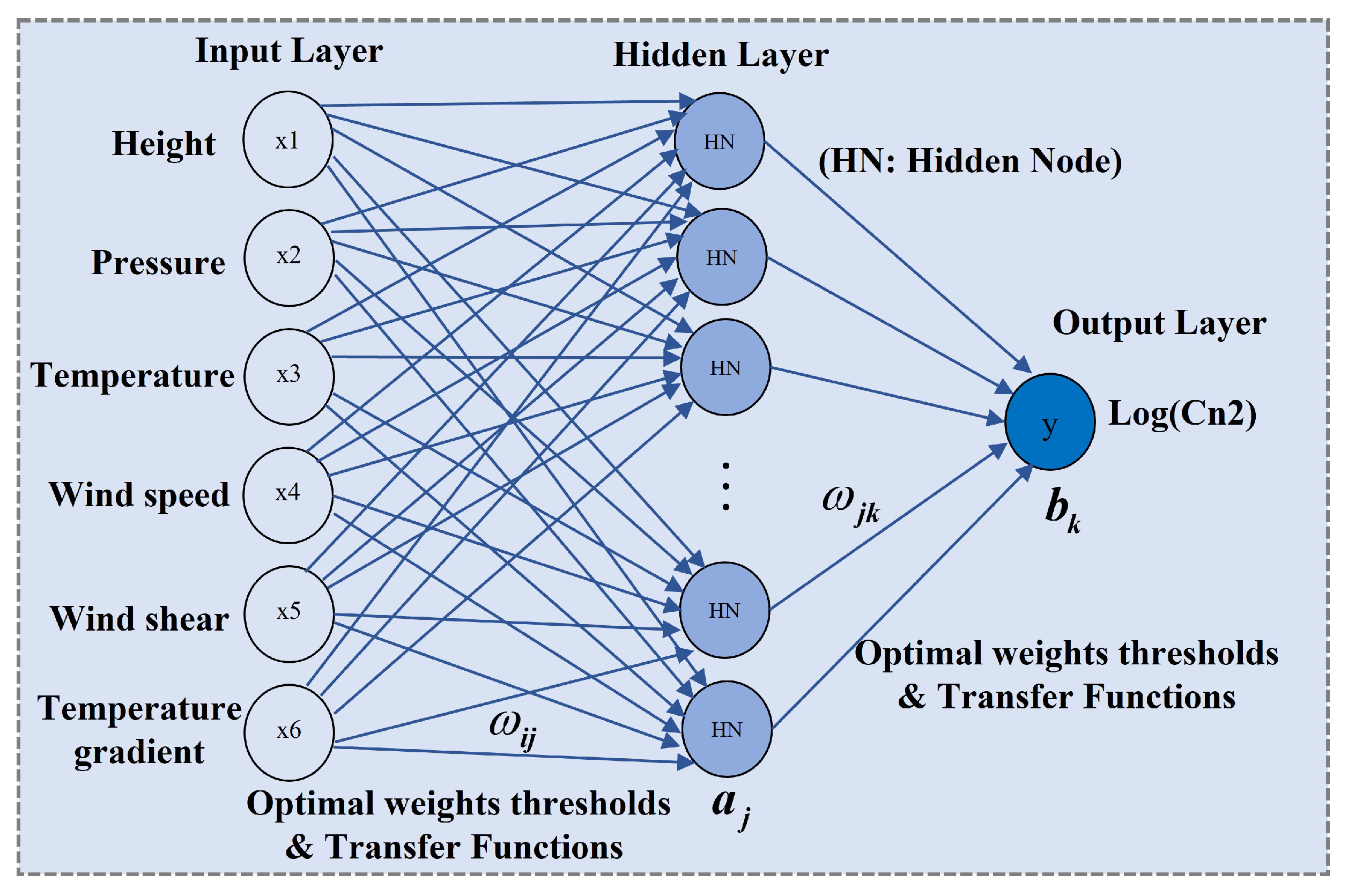
- Confirm the topological structure of GA-BP neural network (M-l-m) and normalize the original data.where x denotes the normalized parameters’ values, which are within the range [−1, 1]. and are the minimum and maximum values of the original parameters data, respectively.
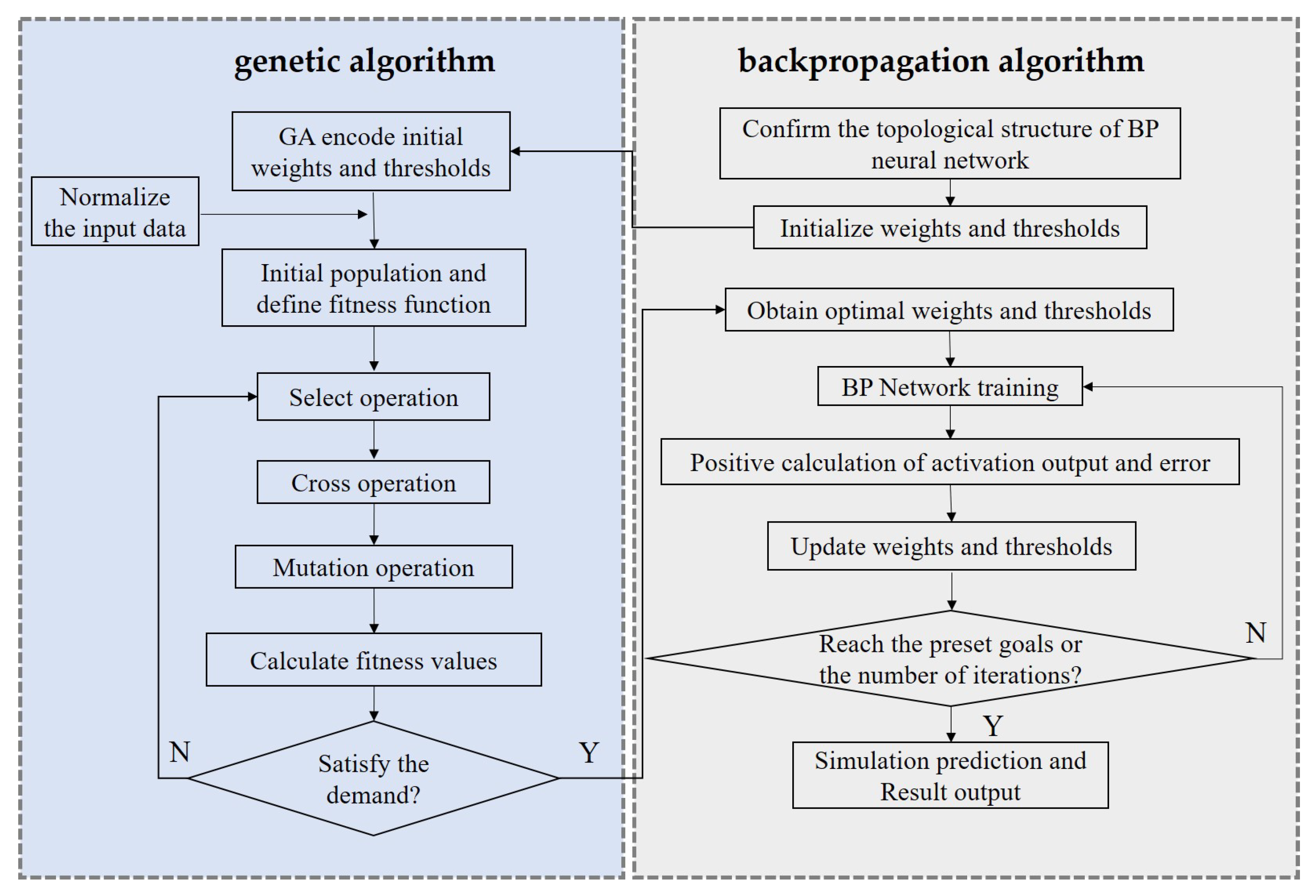
- Code the generation and initialize the population. The random weights , and thresholds , are expressed as chromosome data in the genetic space for coding. Chromosomes containing genetic information are randomly generated, and each data is called an individual, which represents feasible solutions. Genes, namely genetic information, represent components of feasible solutions. The individuals constitute the initial population. Additionally, the length of the Chromosome (C) can be acquired by the number of the input layer (M), the hidden layer (l), and the number of output layer (m).
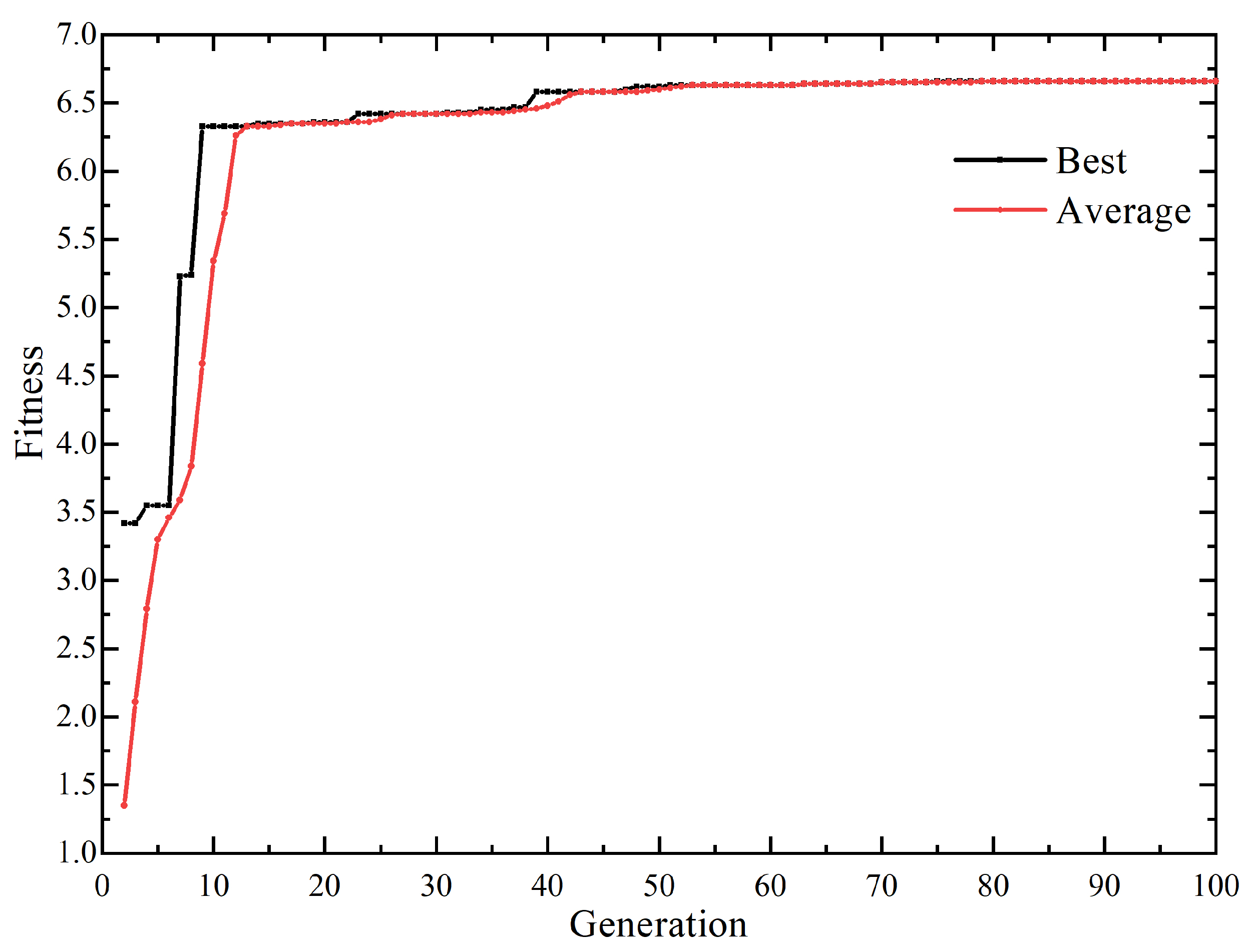
- Fitness assessment. Calculate the fitness (F) of the individual, which is based on the mean absolute error between the actual values and the network output values.where denotes the actual values, denotes the output of the network. N represents the number of training samples. The smaller the mean absolute error, the higher the fitness level.
- Selection, Crossover and Mutation operations: select good individuals from the current population to enter the next generation based on fitness; generate new individuals by using the crossover operation, which combines the characteristics of the parents; the values of chromosomal genes randomly change by mutation operation, providing opportunities for new individuals to emerge.
- The optimal values from GA are assigned as the initial connection weights and thresholds of the BP neural network.
- Calculate the output results of the hidden layer (). can be obtained from the input vector x, the connection weight between the input layer M and the hidden layer l, and the hidden layer threshold .where l denotes the number of hidden layer nodes. f represents the activation function and commonly used sigmoid function as the activation function in GA-BP neural network.
- Calculate the results of the network output layer (). can be calculated based on the output of the hidden layer H, connection weights , and thresholds .
- Calculate network error (). The can be calculated by actual results values () and the network output results ().
- Update weights of the network (, ) according to the network error e.where is the learning rate.
- Update thresholds of the network (, ) based on the network error e.
- If the algorithm reaches the preset goals or reaches the number of iterations, then the network is trained with the training sample; thus, the best-fitting network is created.
- The network is applied to forecast the test samples.
2.2. Physically-Based Model
3. Validation Experiment
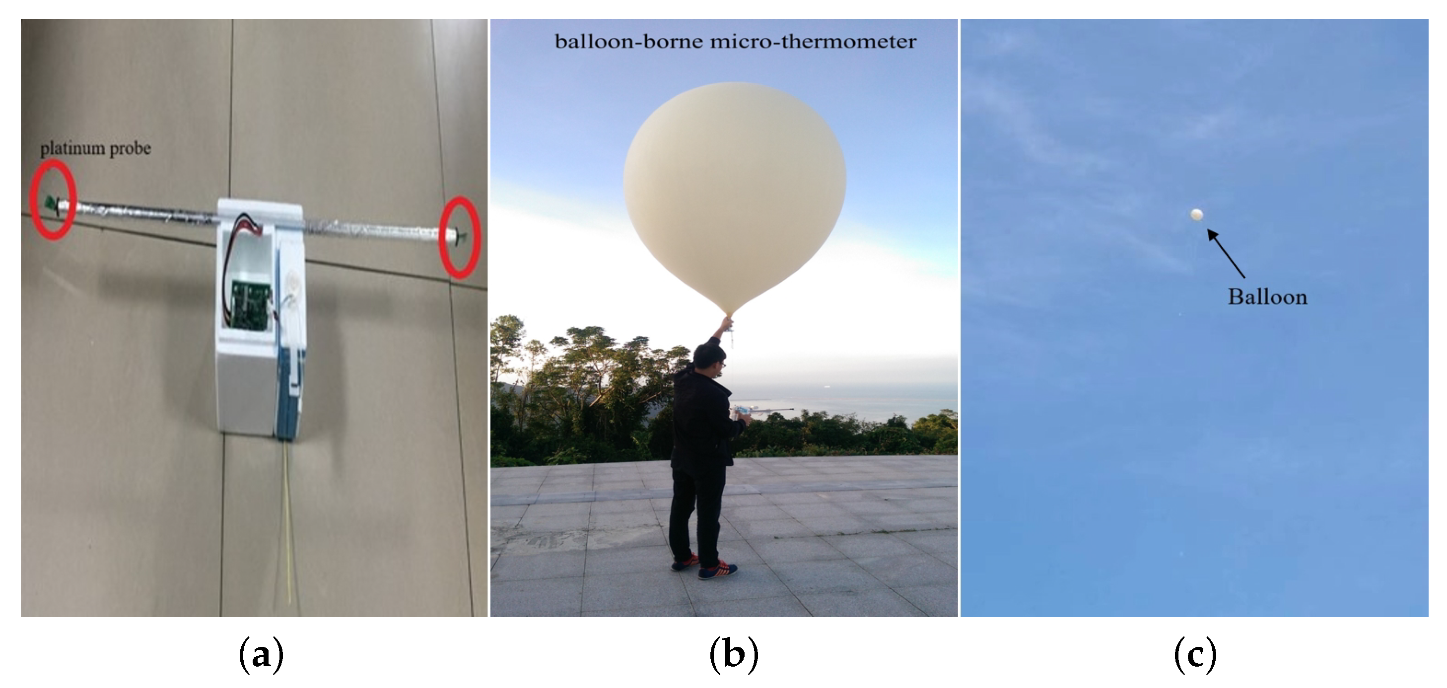
3.1. Balloon-Borne Microthermal Measurement
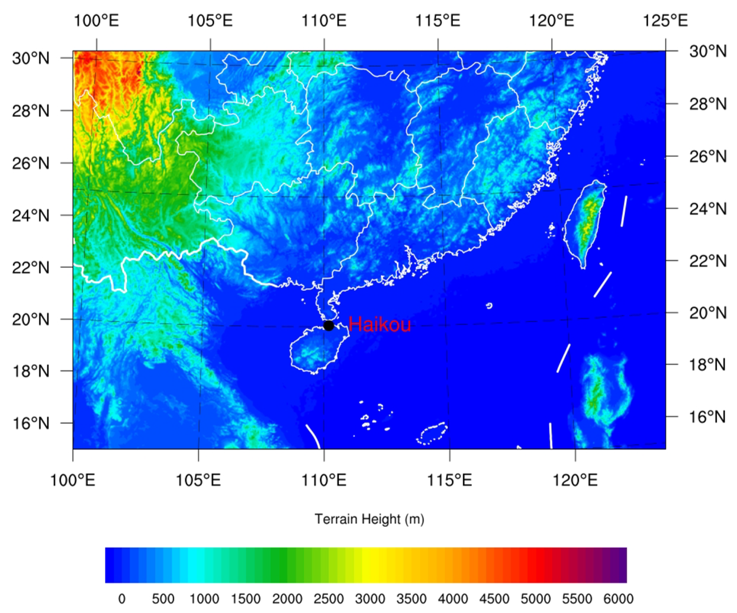
3.2. Field Campaign and Dataset
4. Results
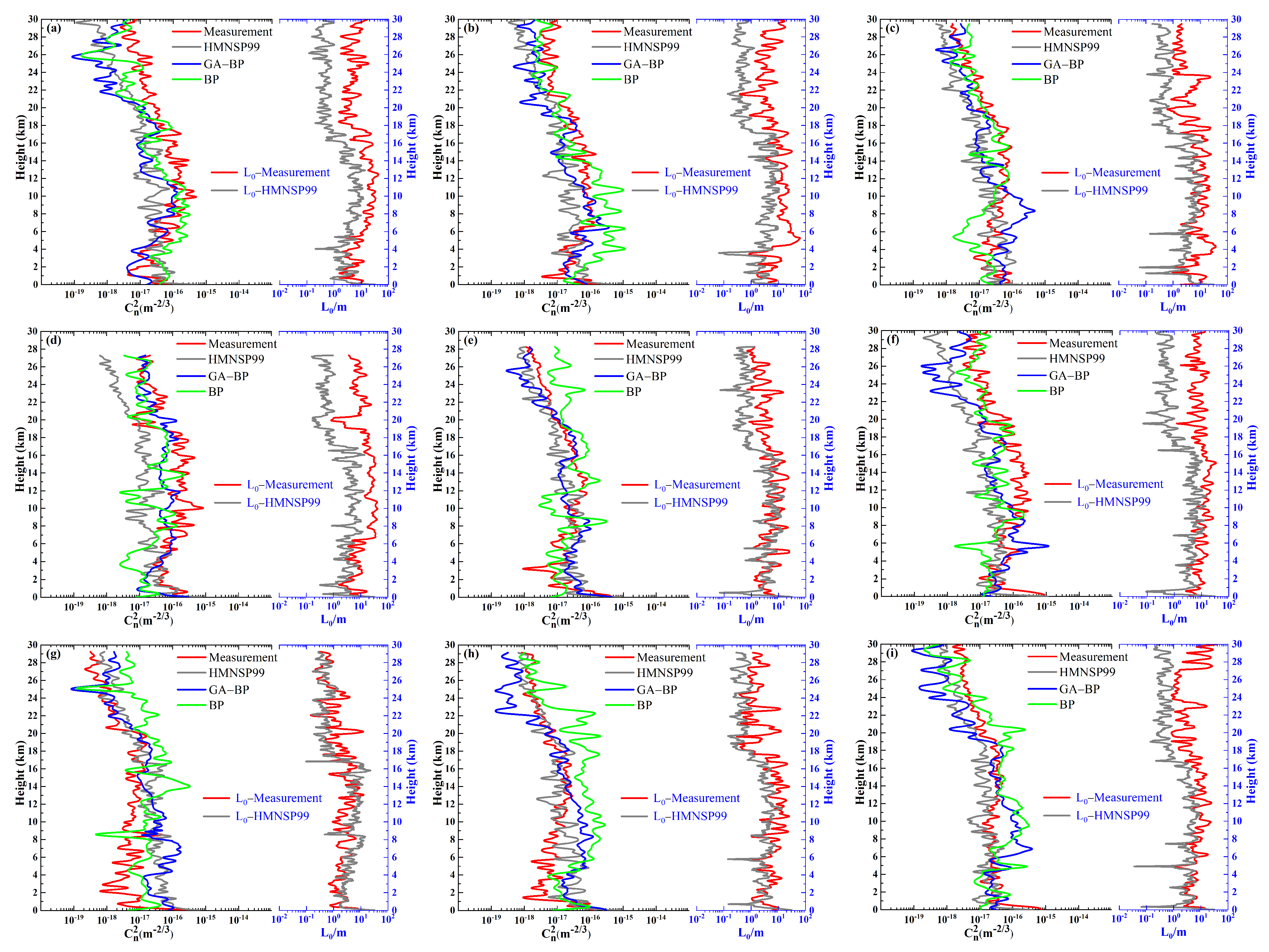
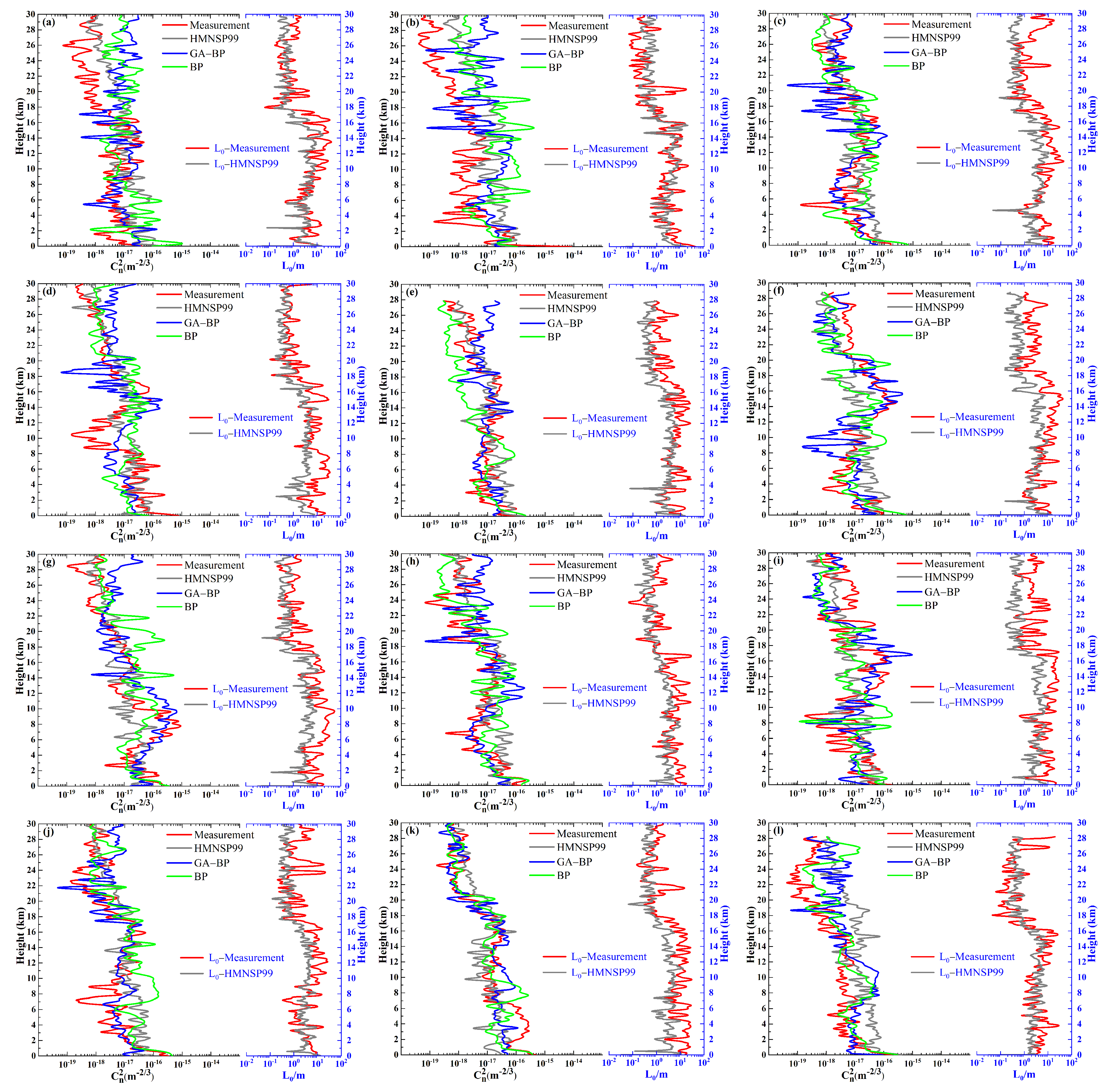
4.1. Estimation of Profiles
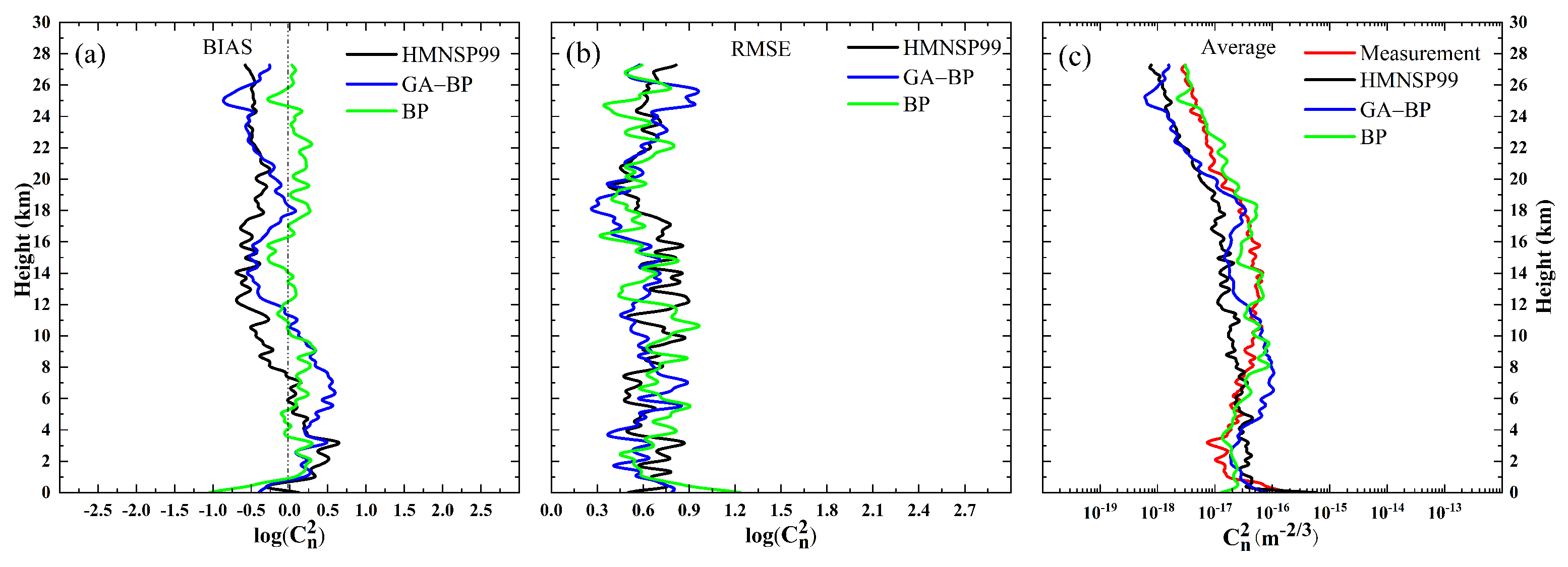
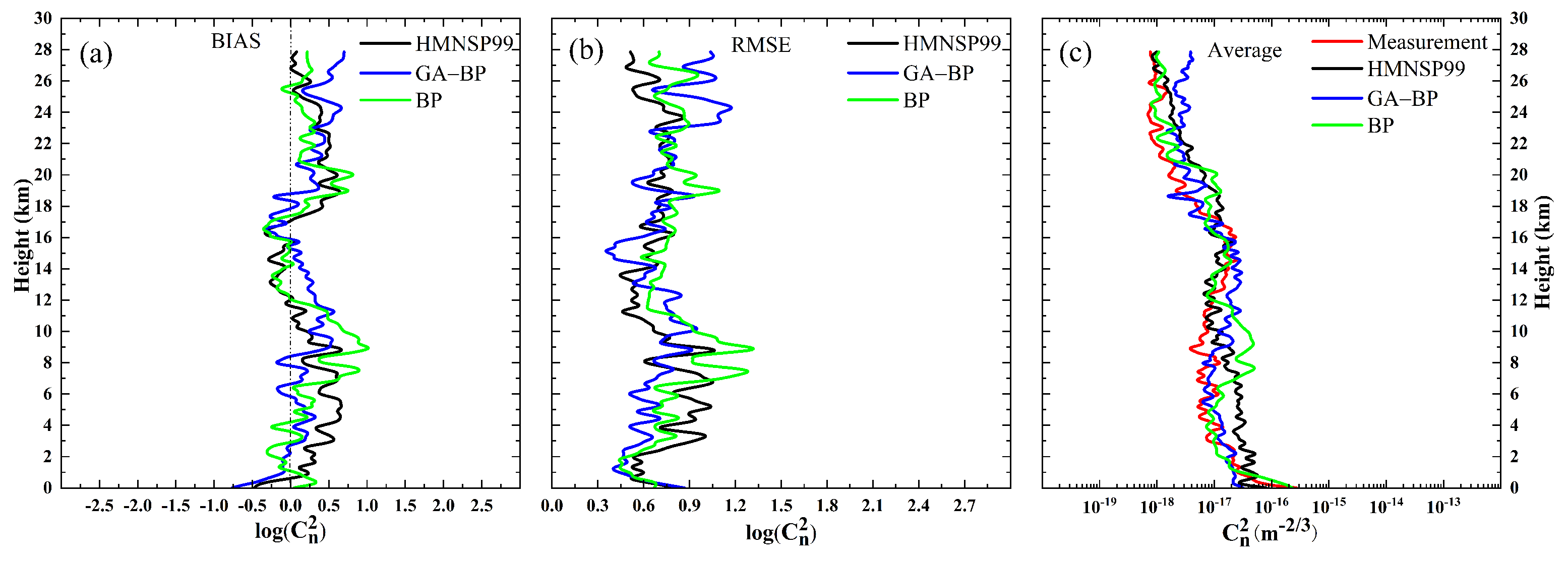
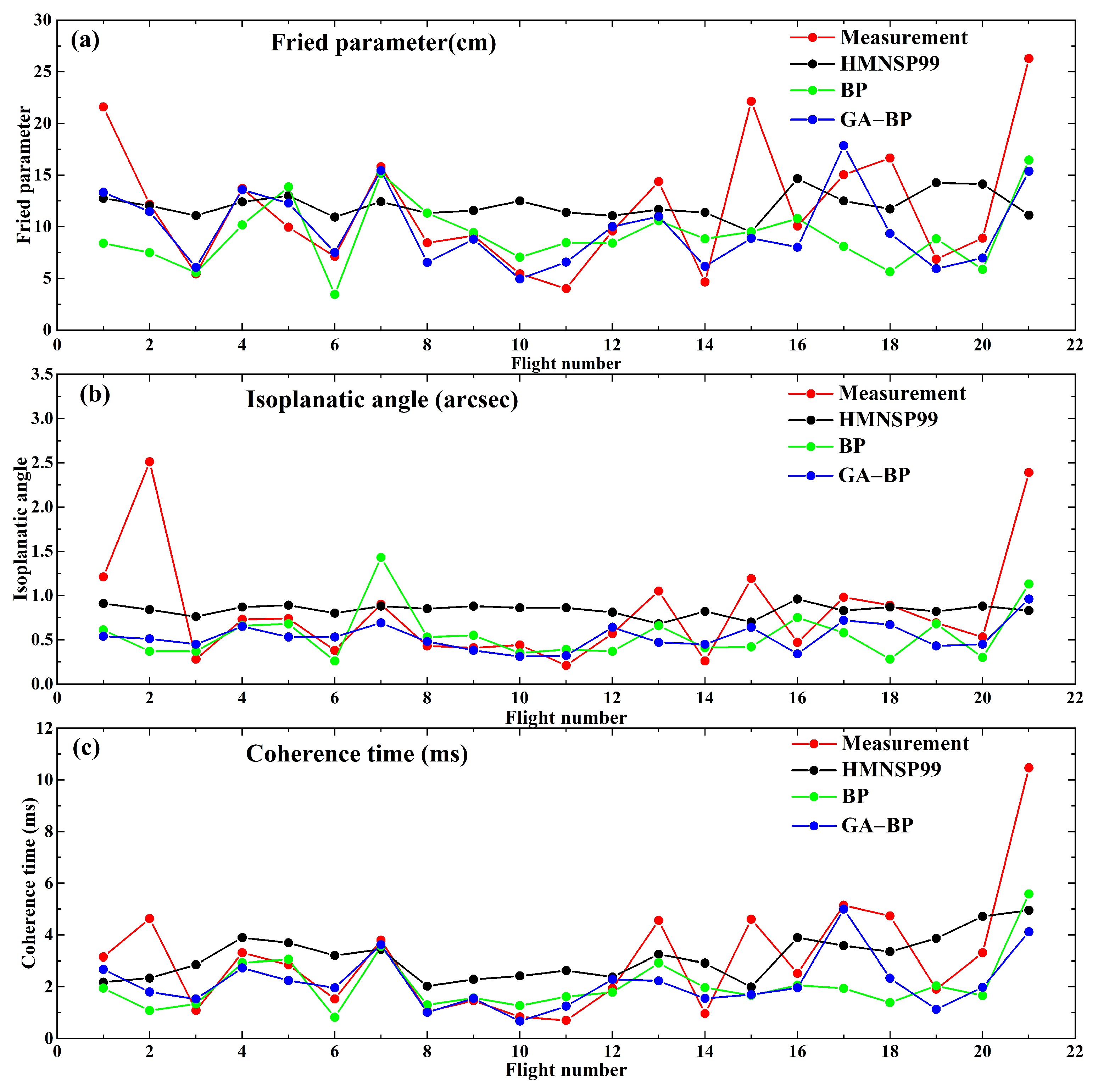
4.2. Error Analysis
5. Discussion
6. Conclusions
Author Contributions
Funding
Data Availability Statement
Acknowledgments
Conflicts of Interest
References
- Tatarskii, V.I. Wave Propagation in a Turbulent Medium; McGraw-Hill: New York, NY, USA, 1961. [Google Scholar]
- Good, R.E.; Beland, R.R.; Murphy, E.A.; Brown, J.H.; Dewan, E.M. Atmospheric models of optical turbulence. In Proceedings of the Modeling of the Atmosphere, Orlando, FL, USA, 4–8 April 1988; pp. 165–186. [Google Scholar]
- Avila, R.; Vernin, J.; Masciadri, E. Whole atmospheric-turbulence profiling with generalized scidar. Appl. Opt. 1997, 36, 7898–7905. [Google Scholar] [CrossRef] [PubMed]
- Kornilov, V.; Tokovinin, A.; Vozyakova, O.; Zaitsev, A.; Shatsky, N.; Potanin, S.; Sarazin, M. MASS: A monitor of the vertical turbulence distribution. In Proceedings of the Astronomical Telescopes and Instrumentation, Waikoloa, HI, USA, 22–28 August 2003; pp. 837–845. [Google Scholar]
- Kornilov, V.; Tokovinin, A.; Shatsky, N.; Voziakova, O.; Potanin, S.; Safonov, B. Combined MASS–DIMM instruments for atmospheric turbulence studies. Mon. Not. R. Astron. Soc. 2007, 382, 1268–1278. [Google Scholar] [CrossRef] [Green Version]
- Vernin, J.; Roddier, F. Experimental determination of two-dimensional spatiotemporal power spectra of stellar light scintillation Evidence for a multilayer structure of the air turbulence in the upper troposphere. J. Opt. Soc. Am. 1973, 63, 270–273. [Google Scholar] [CrossRef]
- Wilson, R.W. SLODAR: Measuring optical turbulence altitude with a Shack–Hartmann wavefront sensor. Mon. Not. R. Astron. Soc. 2002, 337, 103–108. [Google Scholar] [CrossRef] [Green Version]
- Butterley, T.; Wilson, R.W.; Sarazin, M. Determination of the profile of atmospheric optical turbulence strength from SLODAR data. Mon. Not. R. Astron. Soc. 2006, 369, 835–845. [Google Scholar] [CrossRef] [Green Version]
- Vedrenne, N.; Michau, V.; Robert, C.; Conan, J.-M. Improvements in Cn2 profile monitoring with a Shack Hartmann Wavefront sensor. In Proceedings of the Atmospheric Optical Modeling, Measurement, and Simulation II, San Diego, CA, USA, 13–17 August 2006; p. 63030C. [Google Scholar]
- Wang, Z.; Zhang, L.; Kong, L.; Bao, H.; Guo, Y.; Rao, X.; Zhong, L.; Zhu, L.; Rao, C. A modified S-DIMM+: Applying additional height grids for characterizing daytime seeing profiles. Mon. Not. R. Astron. Soc. 2018, 478, 1459–1467. [Google Scholar] [CrossRef]
- Carlisle, E.; Schmidt, D.; Marino, J.; Guesalaga, A. Use of SLODAR for daytime turbulence profiling. In Proceedings of the Adaptive Optics for Extremely Large Telescopes, Tenerife, Canary Islands, Spain, 25–30 June 2017. [Google Scholar]
- Sauvage, C.; Robert, C.; Mugnier, L.M.; Conan, J.-M.; Cohard, J.-M.; Nguyen, K.-L.; Irvine, M.; Lagouarde, J.-P. Near ground horizontal high resolution Cn2 profiling from Shack–Hartmann slopeand scintillation data. Appl. Opt. 2021, 60, 10499–10519. [Google Scholar] [CrossRef]
- Laidlaw, D.J.; Reeves, A.P.; Singhal, H.; Calvo, R.M. Characterizing turbulence profile layers through celestial single-source observations. Appl. Opt. 2022, 61, 498–504. [Google Scholar] [CrossRef]
- Gimmestad, G.G.; Roberts, D.W.; Stewart, J.M.; Wood, J.W.; Eaton, F.D. Testing of LIDAR system for turbulence profiles. In Proceedings of the SPIE Defense and Security Symposium, Orlando, FL, USA, 16–20 March 2008; p. 695109. [Google Scholar]
- Odintsov, S.L.; Gladkikh, V.A.; Kamardin, A.P.; Nevzorova, I.V. Determination of the Structural Characteristic of the Refractive Index of Optical Waves in the Atmospheric Boundary Layer with Remote Acoustic Sounding Facilities. Atmosphere 2019, 10, 711. [Google Scholar] [CrossRef] [Green Version]
- Azouit, M.; Vernin, J. Optical Turbulence Profiling with Balloons Relevant to Astronomy and Atmospheric Physics. Publ. Astron. Soc. Pac. 2005, 117, 536–543. [Google Scholar] [CrossRef]
- Hufnagel, R.E.; Stanley, N.R. Modulation Transfer Function Associated with Image Transmission through Turbulent Media. J. Opt. Soc. Am. 1964, 54, 52–61. [Google Scholar] [CrossRef]
- Abahamid, A.; Jabiri, A.; Vernin, J.; Benkhaldoun, Z.; Azouit, M.; Agabi, A. Optical turbulence modeling in the boundary layer and free atmosphere using instrumented meteorological balloons. Astron. Astrophys. 2004, 416, 1193–1200. [Google Scholar] [CrossRef] [Green Version]
- Nath, D.; Venkat Ratnam, M.; Patra, A.; Krishna Murthy, B.; Bhaskar Rao, S.V. Turbulence characteristics over tropical station Gadanki (13.5 N, 79.2 E) estimated using high-resolution GPS radiosonde data. J. Geophys. Res. 2010, 115, D07102. [Google Scholar] [CrossRef]
- Dewan, E.M.; Good, R.E.; Beland, B.; Brown, J. A Model for (Optical Turbulence) Profiles Using Radiosonde Data; Phillips Laboratory Technical Report, PL-TR-93-2043, ADA 279399; Phillips Laboratory: Albuquerque, NM, USA, 1993. [Google Scholar]
- Ruggiero, F.H.; DeBenedictis, D.A. Forecasting optical turbulence from mesoscale numerical weather prediction models. In Proceedings of the DoD High Performance Modernization Program Users Group Conference, Austin, TX, USA, 1 January 2002; pp. 10–14. [Google Scholar]
- Basu, S. A simple approach for estimating the refractive index structure parameter () profile in the atmosphere. Opt. Lett. 2015, 40, 4130–4133. [Google Scholar] [CrossRef]
- Tracey, B.D.; Duraisamy, K.; Alonso, J.J. A machine learning strategy to assist turbulence model development. In Proceedings of the 53rd AIAA aerospace sciences meeting, Kissimmee, FL, USA, 5–9 January 2015; American Institute of Aeronautics and Astronautics: Reston, VA, USA, 2015; p. 1287. [Google Scholar]
- Pelliccioni, A.; Tirabassi, T. Air dispersion model and neural network: A new perspective for integrated models in the simulation of complex situations. Environ. Modell. Softw. 2006, 21, 539–546. [Google Scholar] [CrossRef]
- Lohani, S.; Glasser, R.T. Turbulence correction with artificial neural networks. Opt. Lett. 2018, 43, 2611–2614. [Google Scholar] [CrossRef]
- Khashei, M.; Rafiei, F.M.; Bijari, M. Hybrid Fuzzy Auto-Regressive Integrated Moving Average (FARIMAH) Model for Forecasting the Foreign Exchange Markets. Int. J. Comput. Int. Syst. 2013, 6, 954–968. [Google Scholar] [CrossRef] [Green Version]
- Gómez, S.L.S.; González-Gutiérrez, C.; Alonso, E.D.; Santos, J.D.; Rodríguez, M.L.S.; Morris, T.; Osborn, J.; Basden, A.; Bonavera, L.; González, J.G.N. Experience with artificial neural networks applied in multi-object adaptive optics. Publ. Astron. Soc. Pac. 2019, 131, 108012. [Google Scholar] [CrossRef]
- Wang, Y.; Basu, S. Using an artificial neural network approach to estimate surface-layer optical turbulence at Mauna Loa, Hawaii. Opt. Lett. 2016, 41, 2334–2337. [Google Scholar] [CrossRef]
- Su, C.D.; Wu, X.Q.; Luo, T.; Wu, S.; Qing, C. Adaptive niche-genetic algorithm based on backpropagation neural network for atmospheric turbulence forecasting. Appl. Opt. 2020, 59, 3699–3705. [Google Scholar] [CrossRef]
- Xu, M.M.; Shao, S.Y.; Liu, Q.; Sun, G.; Han, Y.; Weng, N.Q. Optical Turbulence Profile Forecasting and Verification in the Offshore Atmospheric Boundary Layer. Appl. Sci. 2021, 11, 8523. [Google Scholar] [CrossRef]
- Aslanargun, A.; Mammadov, M.; Yazici, B.; Yolacan, S. Comparison of ARIMA, neural networks and hybrid models in time series: Tourist arrival forecasting. J. Stat. Comput. Simul. 2007, 77, 29–53. [Google Scholar] [CrossRef]
- Ranjithan, S.; Eheart, J.W.; Garrett, J.H., Jr. Neural network-based screening for groundwater reclamation under uncertainty. Water Resour. Res. 1993, 29, 563–574. [Google Scholar] [CrossRef]
- Riedmiller, M.; Braun, H. A direct adaptive method for faster backpropagation learning: The RPROP algorithm. In Proceedings of the IEEE International Conference on Neural Networks, San Francisco, CA, USA, 28 March–1 April 1993; pp. 586–591. [Google Scholar]
- Bufton, J.L. Correlation of microthermal turbulence data with meteorological soundings in the troposphere. J. Atmos. Sci. 1973, 30, 83–87. [Google Scholar] [CrossRef]
- Qing, C.; Wu, X.Q.; Li, X.B.; Luo, T.; Su, C.D.; Zhu, W.Y. Mesoscale optical turbulence simulations above Tibetan Plateau: First attempt. Opt. Express 2020, 28, 4571–4586. [Google Scholar] [CrossRef]
- Qing, C.; Luo, T.; Bi, C.C.; Li, X.B.; Cui, S.C.; Yang, Q.K.; Su, C.D.; Wu, S.; Qian, X.M.; Wu, X.Q. Optical turbulence and wind speed distributions above the Tibetan Plateau from balloon-borne microthermal measurements. Mon. Not. R. Astron. Soc. 2021, 508, 4096–4105. [Google Scholar] [CrossRef]
- Bi, C.C.; Qian, X.M.; Liu, Q.; Zhu, W.Y.; Li, X.B.; Luo, T.; Wu, X.Q.; Qing, C. Estimating and measurement of atmospheric optical turbulence according to balloon-borne radiosonde for three sites in China. J. Opt. Soc. Am. A 2020, 37, 1785–1794. [Google Scholar] [CrossRef]
- Han, Y.J.; Wu, X.Q.; Luo, T.; Qing, C.; Yang, Q.K.; Jin, X.M.; Liu, N.N.; Wu, S.; Su, C.D. New () statistical model based on first radiosonde turbulence observation over Lhasa. J. Opt. Soc. Am. A 2020, 37, 995–1001. [Google Scholar] [CrossRef]
- Beland, R.R. Propagation through atmospheric optical turbulence. Atmos. Propag. Radiat. 1993, 2, 157–232. [Google Scholar]
- Basu, S.; Osborn, J.; He, P.; DeMarco, A. Mesoscale modelling of optical turbulence in the atmosphere: The need for ultrahigh vertical grid resolution. Mon. Not. R. Astron. Soc. 2020, 497, 2302–2308. [Google Scholar] [CrossRef]
- McHugh, J.P.; Jumper, G.Y.; Chun, M. Balloon thermosonde measurements over Mauna Kea and comparison with seeing measurements. Publ. Astron. Soc. Pac. 2008, 120, 1318–1324. [Google Scholar] [CrossRef]
- Masciadri, E.; Stoesz, J.; Hagelin, S.; Lascaux, F. Optical turbulence vertical distribution with standard and high resolution at Mt Graham. Mon. Not. R. Astron. Soc. 2010, 404, 144–158. [Google Scholar]
- Roddier, F.; Gilli, J.M.; Lund, G. On the origin of speckle boiling and its effects in stellar speckle interferometry. J. Opt. 1982, 13, 263–271. [Google Scholar] [CrossRef]
- Masciadri, E.; Lascaux, F.; Fini, L. MOSE: Operational forecast of the optical turbulence and atmospheric parameters at European Southern Observatory ground-based sites—I. Overview and vertical stratification of atmospheric parameters at 0–20 km. Mon. Not. R. Astron. Soc. 2013, 436, 1968–1985. [Google Scholar] [CrossRef] [Green Version]
- Hagelin, S.; Masciadri, E.; Lascaux, F. Optical turbulence simulations at Mt Graham using the Meso-NH model. Mon. Not. R. Astron. Soc. 2011, 412, 2695–2706. [Google Scholar] [CrossRef] [Green Version]
- Jellen, C.; Burkhardt, J.; Brownell, C.; Nelson, C. Machine learning informed predictor importance measures of environmental parameters in maritime optical turbulence. Appl. Opt. 2020, 59, 6379–6389. [Google Scholar] [CrossRef]


| Parameter | Measuring Range | Accuracy |
|---|---|---|
| Temperature | −90–50 °C | 0.2 °C |
| Pressure | 5–1060 hPa | 0.3 hPa |
| Wind speed | 0–150 m·s | 0.3 m·s |
| Wind Direction | 0–360° | 3° |
| Turbulence | 10–10 m | 10 m |
| Flight | Launch | Launch | Termination | Termination |
|---|---|---|---|---|
| Number | Date (LT) | Time (LT) | Time (LT) | Altitude (m) |
| 1 | 28 March 2018 | 19:58 | 21:18 | 29,860 |
| 2 | 29 March 2018 | 20:01 | 21:23 | 32,030 |
| 3 | 1 April 2018 | 07:44 | 09:06 | 30,230 |
| 4 | 1 April 2018 | 20:15 | 21:42 | 31,150 |
| 5 | 2 April 2018 | 19:50 | 21:25 | 32,590 |
| 6 | 3 April 2018 | 07:50 | 09:19 | 30,070 |
| 7 | 3 April 2018 | 19:50 | 21:05 | 27,860 |
| 8 | 8 April 2018 | 07:52 | 09:22 | 29,500 |
| 9 | 9 April 2018 | 19:50 | 21:06 | 28,770 |
| 10 | 10 April 2018 | 20:00 | 21:37 | 33,030 |
| 11 | 11 April 2018 | 08:00 | 09:18 | 27,290 |
| 12 | 12 April 2018 | 08:00 | 09:23 | 28,270 |
| 13 | 13 April 2018 | 20:00 | 21:34 | 32,510 |
| 14 | 14 April 2018 | 08:00 | 09:29 | 30,360 |
| 15 | 20 April 2018 | 08:00 | 09:18 | 29,250 |
| 16 | 20 April 2018 | 20:01 | 21:28 | 30,410 |
| 17 | 21 April 2018 | 20:01 | 21:29 | 31,490 |
| 18 | 22 April 2018 | 08:00 | 09:27 | 29,150 |
| 19 | 22 April 2018 | 20:00 | 21:32 | 31,650 |
| 20 | 23 April 2018 | 08:00 | 09:25 | 32,250 |
| 21 | 27 April 2018 | 01:40 | 02:57 | 28,210 |
| Flight | () | () | () | |||
|---|---|---|---|---|---|---|
| Number | BP | GA-BP | BP | GA-BP | BP | GA-BP |
| 1 | −13.19 | −8.27 | −0.6 | −0.67 | −1.2 | −0.47 |
| 2 | −4.69 | −0.72 | −2.14 | −2 | −3.55 | −2.83 |
| 3 | 0.12 | 0.63 | 0.09 | 0.17 | 0.25 | 0.44 |
| 4 | −3.55 | −0.14 | 0.07 | −0.08 | −0.39 | −0.58 |
| 5 | 3.91 | 2.34 | −0.06 | −0.21 | 0.21 | −0.61 |
| 6 | −3.67 | 0.39 | −0.12 | 0.15 | −0.71 | 0.43 |
| 7 | −0.66 | −0.37 | 0.53 | −0.21 | −0.24 | −0.17 |
| 8 | 2.87 | −1.97 | 0.1 | 0.05 | 0.26 | −0.03 |
| 9 | 0.3 | −0.35 | 0.14 | −0.03 | 0.1 | 0.08 |
| 10 | 1.6 | −0.5 | −0.09 | −0.13 | 0.43 | −0.17 |
| 11 | 4.45 | 2.56 | 0.18 | 0.11 | 0.92 | 0.55 |
| 12 | −1.18 | 0.42 | −0.2 | 0.07 | −0.15 | 0.35 |
| 13 | −3.79 | −3.38 | −0.39 | −0.58 | −1.64 | −2.33 |
| 14 | 4.19 | 1.52 | 0.15 | 0.19 | 1.01 | 0.59 |
| 15 | −12.63 | −13.26 | −0.77 | −0.55 | −2.93 | −2.9 |
| 16 | 0.72 | −2.06 | 0.28 | −0.13 | −0.46 | −0.56 |
| 17 | −6.94 | 2.81 | −0.4 | −0.26 | −3.2 | −0.15 |
| 18 | −11 | −7.3 | −0.61 | −0.22 | −3.34 | −2.4 |
| 19 | 1.98 | −0.93 | −0.01 | −0.26 | 0.13 | −0.78 |
| 20 | −3.02 | −1.92 | −0.23 | −0.08 | −1.65 | −1.33 |
| 21 | −9.84 | −10.92 | −1.26 | −1.43 | −4.89 | −6.35 |
Publisher’s Note: MDPI stays neutral with regard to jurisdictional claims in published maps and institutional affiliations. |
© 2022 by the authors. Licensee MDPI, Basel, Switzerland. This article is an open access article distributed under the terms and conditions of the Creative Commons Attribution (CC BY) license (https://creativecommons.org/licenses/by/4.0/).
Share and Cite
Bi, C.; Qing, C.; Wu, P.; Jin, X.; Liu, Q.; Qian, X.; Zhu, W.; Weng, N. Optical Turbulence Profile in Marine Environment with Artificial Neural Network Model. Remote Sens. 2022, 14, 2267. https://0-doi-org.brum.beds.ac.uk/10.3390/rs14092267
Bi C, Qing C, Wu P, Jin X, Liu Q, Qian X, Zhu W, Weng N. Optical Turbulence Profile in Marine Environment with Artificial Neural Network Model. Remote Sensing. 2022; 14(9):2267. https://0-doi-org.brum.beds.ac.uk/10.3390/rs14092267
Chicago/Turabian StyleBi, Cuicui, Chun Qing, Pengfei Wu, Xiaomei Jin, Qing Liu, Xianmei Qian, Wenyue Zhu, and Ningquan Weng. 2022. "Optical Turbulence Profile in Marine Environment with Artificial Neural Network Model" Remote Sensing 14, no. 9: 2267. https://0-doi-org.brum.beds.ac.uk/10.3390/rs14092267