A Continuous Change Tracker Model for Remote Sensing Time Series Reconstruction

Abstract

It is hard for current time series reconstruction methods to achieve the balance of high-precision time series reconstruction and explanation of the model mechanism. The goal of this paper is to improve the reconstruction accuracy with a well-explained time series model. Thus, we developed a function-based model, the CCTM (Continuous Change Tracker Model) model, that can achieve high precision in time series reconstruction by tracking the time series variation rate. The goal of this paper is to provide a new solution for high-precision time series reconstruction and related applications. To test the reconstruction effects, the model was applied to four types of datasets: normalized difference vegetation index (NDVI), gross primary productivity (GPP), leaf area index (LAI), and MODIS surface reflectance (MSR). Several new observations are as follows. First, the CCTM model is well explained and based on the second-order derivative theorem, which divides the yearly time series into four variation types including uniform variations, decelerated variations, accelerated variations, and short-periodical variations, and each variation type is represented by a designed function. Second, the CCTM model provides much better reconstruction results than the Harmonic model on the NDVI, GPP, MSR, and LAI datasets for the seasonal segment reconstruction. The combined use of the Savitzky–Golay filter and the CCTM model is better than the combinations of the Savitzky–Golay filter with other models. Third, the Harmonic model has the best trend-fitting ability on the yearly time series dataset, with the highest R-Square and the lowest RMSE among the four function fitting models. However, with seasonal piecewise fitting, the four models all achieved high accuracy, and the CCTM performs the best. Fourth, the CCTM model should also be applied to time series image compression, two compression patterns with 24 coefficients and 6 coefficients respectively are proposed. The daily MSR dataset can achieve a compression ratio of 15 by using the 6-coefficients method. Finally, the CCTM model also has the potential to be applied to change detection, trend analysis, and phenology and seasonal characteristics extractions.

1. Introduction

Remote sensing datasets provide long records of earth observation, which are essential for earth sciences research. Since the 1960s, remote sensing satellite datasets (e.g., NOAA/AVHRR, MODIS, Landsat) have been widely applied to the study of global environmental change [1,2,3,4]. With the development of remote sensing retrieval algorithms, a series of land surface variables products have been archived, such as the normalized difference vegetation index (NDVI), leaf area index (LAI), gross primary productivity (GPP), and atmospherically corrected surface reflectance [5,6,7].

Nonetheless, the time series land surface variables are not always evenly distributed and continuous due to cloud, cloud shadows, snow contamination, low temporal frequency, sun-sensor-surface viewing geometry of different seasons, different sensors and sensor failure, etc. High-precision land cover classification, monitoring, and trend analysis all require continuous fine-scale Remotely Sensed Land Surface Products (RSLSP) [8,9,10,11,12,13]. To obtain temporally and spatially continuous RSLSP datasets, spatial-, spectral-, and temporal-based methods and their combinations (e.g., joint spatio-spectral methods and joint spatio-temporal methods) for the time series reconstruction of RSLSP have been proposed [10].

The temporal-based methods have been widely used to remove noises in the time series reconstruction, which can be categorized into five categories [14]: (1) temporal interpolation methods, (2) temporal filters, (3) temporal function-fitting methods, (4) temporal deep learning methods and (5) frequency-based methods.

The temporal interpolation methods like Maximum Value Composite (MVC) [15,16,17], iterative interpolation for data reconstruction (IDR) [18], data assimilation (DA) [19,20,21] and the best index slope extraction (BISE) [22,23] have been commonly applied to filling time series gaps. However, such algorithms are not suitable for the reconstruction of data with long-term gaps. Due to no consideration of atmosphere interference, the MVC method can lead to the loss of useful temporal information. The IDR method proves prone to overestimating the time series values during the vegetation dormant periods [24]. The DA method has poor performance at the onset of vegetation spring green [20], and the BISE method is bad for long-term decline trends [25].

As for the temporal filter methods, there are the Savitzky-Golay (SG) filter, the Mean-Value iterative (MVI) filter, the Moving Average Filter, and the Changing Weight Filter. The famous Savitzky–Golay (SG) filter method has been widely applied to remove temporal noises from the NDVI, GPP, and reflectance time series [26,27]. However, the processing effect of the SG filter method is highly dependent on the size of the filtering window size. A large window size can also lead to the existing variations being smoothed out, and a small window size can not effectively reduce the noises in the time series [28,29]. The MVI filter has negative effects for areas with high interannual changes, and the MA filter will change the width and the height of the curve, for the CW method, the remaining noises in the time series can be problematic.

The temporal function fitting method reconstructs the time series by stimulating the time-series variation with parameterized functions. The asymmetric Gaussian (AG) model can extract the phonological parameters during the smoothing process. However, it will lead to a loss of details about vegetation changes if there is a lot of noise in the original time series [30,31]. The double logistic (DL) technique is effective for revealing the trend of the NDVI time series, but it remains problematic with NDVI in winter [32].

Among frequency-based techniques, the Fourier transform is very effective in processing periodic time-series signals, as it can decompose them into amplitude and phase information, but it has poor performance for irregular time series due to the strict symmetry of the formula [33,34]. The wavelet transform (WT) method also easily ignores the reasonable high values when there are frequent variations in the time series [35].

The harmonic analysis of time series (HANTS) method was later proposed by Verhoef [36] and has been widely used to reconstruct time-series datasets of the NDVI, LAI, and land surface temperatures (LSTs) [37,38,39]. The method has also been successfully used to predict Landsat values at any given time and has achieved relatively high accuracy in Landsat data reconstruction [9]. However, the HANTS may result in a large deviation from the original time series if there are long-term data gaps [40].

In this paper, a hybrid time series reconstruction method has been proposed. Several time series outlier recognition and gap-filling methods have been applied to fill the long-term gaps. A high-precision model continuous change rate tracking model (CCTM) has been developed for the reconstruction of time series RSLSP. The CCTM model divides the yearly time series into four seasons and reconstructs each seasonal time series with a least-squares solver. The CCTM model decomposes the land surface variations into four parts by the variation types: uniform variation part, accelerated variation part, decelerated variation part, and short-term periodic variation part. Every part is represented by a designed function. In addition, the SG filter is adapted for LAI, GPP, and surface reflectance time series data to effectively control the degree of smoothing and retain the original characteristics by setting limited iteration times or adding smoothing controlling parameters.

Current time series reconstruction methods do have their advantages, but the long-term gaps, over-fitting, and remaining noise issues are still disturbing [41]. More importantly, none of the methods above can precisely predict the time series values on a daily scale. The objectives of this paper are: (1) to provide solutions to the time series deficiencies of long-term gaps, over-fitting, and remaining noise issues; and (2) to develop a comprehensive continuous time series reconstruction method that can precisely predict time series values.

2. Materials and Methods

2.1. Data

A series of land surface variable datasets were chosen to evaluate the reconstruction performance of the new model. The NDVI (produced by MOD09Q1), LAI (MCD15A3H), GPP (MOD17A2H), and MSR (MOD09Q1) datasets from 2001 to 2005 in the global region are selected. 183 NDVI images, 183 GPP images, 183 MSR images, and 228 LAI images are collected in the global region. The detailed information is shown in

Table 1. Detailed information about the dataset used in the study.

Dataset	Date	URL	Description
MCD15A3H (MODIS Leaf Area Index/FPAR 4-Day Global 500 m)	2001–2005	https://developers.google.com/earth-engine/datasets/catalog/MODIS_006_MCD15A3H (accessed on 21 April 2022)	The MCD15A3H V6 level 4, Combined Fraction of Photosynthetically Active Radiation (FPAR), and Leaf Area Index (LAI) product is a 4-day composite data set with 500 m pixel size.
MOD17A2H (Terra Gross Primary Productivity 8-Day Global 500 M)	2001–2005	https://developers.google.com/earth-engine/datasets/catalog/MODIS_006_MOD17A2H (accessed on 21 April 2022)	The MOD17A2H V6 Gross Primary Productivity (GPP) product is a cumulative 8-day composite with a 500 m resolution.
MOD09Q1 (Terra Surface Reflectance 8-Day Global 250 m)	2001–2005	https://developers.google.com/earth-engine/datasets/catalog/MODIS_006_MOD09Q1 (accessed on 21 April 2022)	The MOD09Q1 product provides an estimate of the surface spectral reflectance of bands 1 and 2 at 250 m resolution and corrected for atmospheric conditions such as gasses, aerosols, and Rayleigh scattering.

. Among them, the NDVI and MSR datasets have temporal and spatial resolutions of 8 days and 250 m, the LAI dataset has temporal and spatial resolutions of 4 days and 500 m, and the GPP dataset has temporal and spatial resolutions of 8 days and 500 m.

The NDVI time series dataset is based on the MOD09Q1 product. MCD15A3H, MOD11A2, MOD17A2H, and MOD09Q1 time-series datasets are provided with detailed quality control instructions. The NDVI, LAI, and GPP products were chosen as they are important in reflecting vegetation changes. The MSR product (including near-infrared and red band data) was chosen as it is a representative primary remote sensing product.

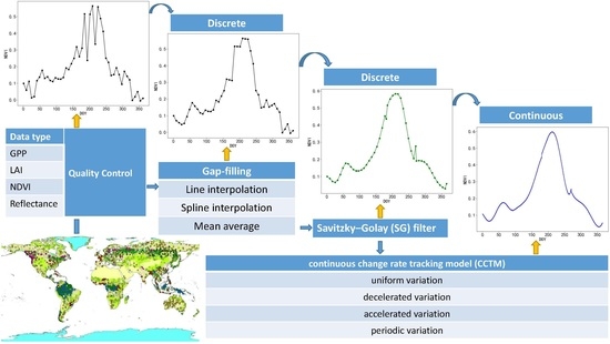
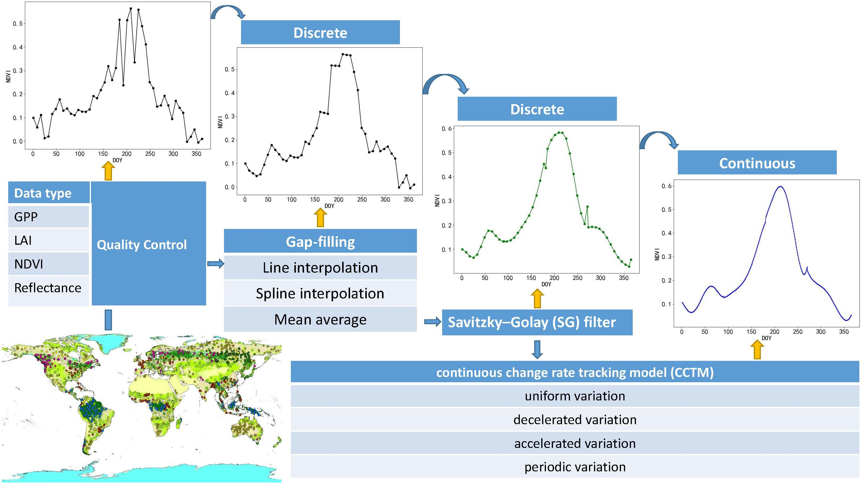
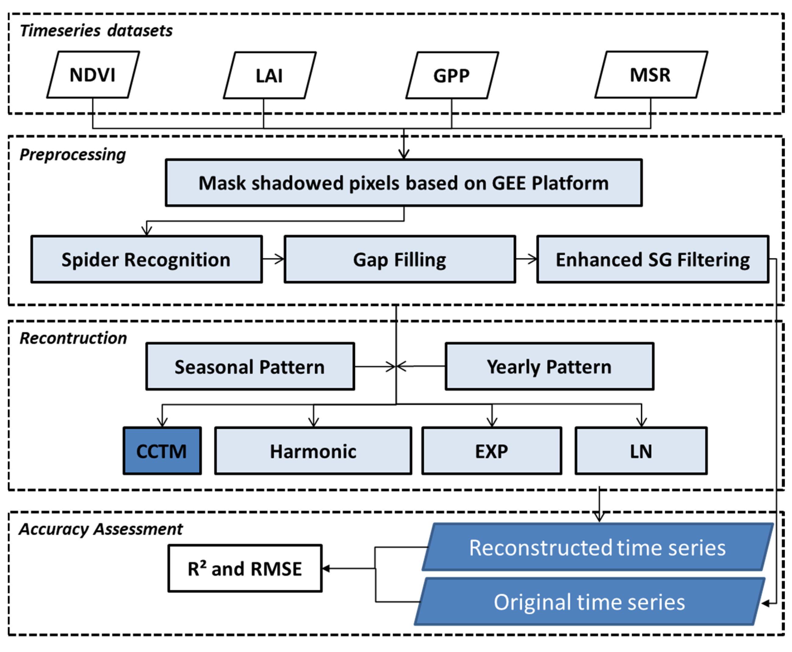
2.2. Time Series Reconstruction Flow

The data processing consists of three parts (Figure 1). (1) Preprocessing includes setting a mask for the dataset according to the quality control information, outlier recognition, gap-filling, and enhanced SG filtering, which is only necessary for time series datasets that contain noise. If >50% of the points in the yearly time series are invalid, the invalid points are filled with zeros, and gap-filling and enhanced SG filtering are not needed. (2) The reconstruction results are compared in seasonal time series patterns and yearly time-series patterns. In the yearly time series pattern, four models are applied to reconstruct the yearly segment time series, but in the seasonal segment time series, four models are separately used to reconstruct every seasonal segment time series.

These four-time series reconstruction models include: (i) the CCTM model developed in this paper, (ii) the Harmonic model (an eight-parameter harmonic model), (iii) EXP (an exponential model), and (iv) LN model (a logarithmic model). (3) Accuracy assessment evaluates the reconstruction accuracy between the original time series processed by SG filter and gap-filling methods and the continuous-time series reconstructed by the four models.

2.3. Data Preprocessing

Data preprocessing involves two parts: (1) point sampling and quality control are conducted on the Google Earth Engine (GEE) platform; and (2) outlier recognition, gap-filling, and enhanced SG filtering are conducted.

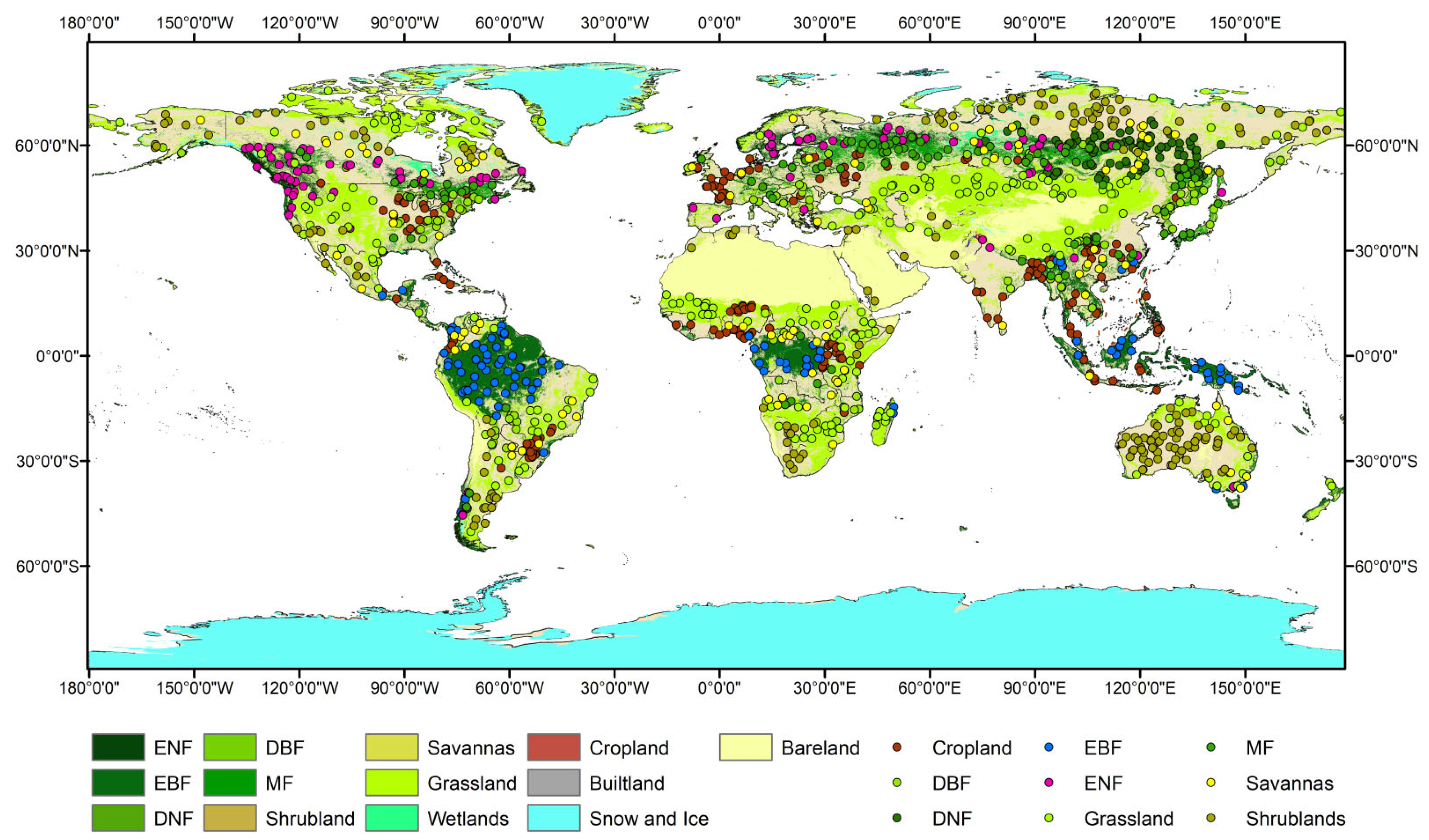
2.3.1. Points Sampling and Quality Control

The six kinds of datasets were processed using the following two steps. First, setting a mask for time series data with the quality control band provides the pixel quality status of each point in the time series. Second, to comprehensively analyze the reconstruction effects on the specific landcover types, the stable land cover type was defined as the land cover which has not been changed from 2001 to 2005, and eight stable land cover types were extracted from the MCD12Q1.006 [42] product for the period 2001–2005: evergreen needleleaf forests (ENF), evergreen broadleaf forests (EBF), deciduous needleleaf forests (DBF), deciduous broadleaf forests (DBF), mixed forests (MF), shrublands, savannas, grasslands, and croplands. Then, we selected 100 sampling points for each of the ENF, EBF, DBF, and MF datasets and 200 sampling points for each of the shrubland, savanna, grassland, and cropland datasets. The distribution of the sampling points and the stable land cover types are shown in Figure 2. The seasons in the northern hemisphere were defined as: winter, 1 December–28 February; spring, 1 March–31 May; summer, 1 June–31 August; and autumn, 1 September–30 November. Southern hemisphere seasons are exactly the opposite. For each sampling point in the different land cover types, five-year time series (2001–2005) were obtained according to these seasonal periods.

Noises in the time series can be reduced by methods, such as the maximum composite method (choosing the highest-quality pixel in a time interval [15]) and the typical time-series filter [36,41,43]. However, there were still spurious points that remained. Since outliers can deviate obviously from a gradually changing time series and always exhibit sudden increases or decreases, a series of algorithms were provided to recognize the spurious points in the time series.

An outlier is defined based on two criteria. The first is that its value is greater/lower than the mean of its moving window plus/minus the cutoff (cutoff is twice the standard deviation of the points in the moving window [43]. In Equation (1), sigma (y(t − c), y(t − c + 1), …, y(t), y(t + 1), …, y(t + c)) is the standard deviation of the point values in the moving window). It is the serial number of time series points, where $y\left(t\right)$ is the value of the tth time series point, c is half of the moving window size, and $2c+1$ is the size of the moving window.

$$\begin{gathered} y\left(t\right)<mean\left(y\left(t-c\right),y\left(t-c+1\right),\dots ,y\left(t\right),y\left(t+1\right),\dots ,y\left(t+c\right)\right)-cutoff \\ y\left(t\right)>mean\left(y\left(t-c\right),y\left(t-c+1\right),\dots ,y\left(t\right),y\left(t+1\right),\dots ,y\left(t+c\right)\right)+cutoff \\ cutof=2\ast sigma\left(y\left(t-c\right),y\left(t-c+1\right),\dots ,y\left(t\right),y\left(t+1\right),\dots ,y\left(t+c\right)\right) \end{gathered}$$

(1)

In Equation (2), $N_K$ is the value of the kth point; $d{N}_{K-1}{N}_K$ is the inclining or declining slope from the (k − 1)th point $N_{K-1}$ to the kth point $N_K$; $d{N}_K{N}_{K+1}$ is the inclining or declining slope from the (k − 1)th point $N_K$ to the kth point $N_{K+1}$; K is the serial number of the time series point; and $ndt$ is the threshold of the time series points whose interval is n-day, which is defined as 30%/16 × n and equal to 30% when the temporal resolution is 16 days. The second criterion is that both $d{N}_{K-1}{N}_K$ and $d{N}_K{N}_{K+1}$ are larger than $ndt$ or lower than $-ndt$.

$$\begin{gathered} d{N}_{K-1}{N}_K=\frac{N_{K-1}-N_K}{N_K}\times 100\% \\ d{N}_K{N}_{K+1}=\frac{N_{K+1}-N_K}{N_K}\times 100\% \\ ndt=30\%/16\times n \end{gathered}$$

(2)

If one of the above criteria is met, the point in the time series is defined as an outlier. The second criterion is always used in the outlier recognition of NDVI time series and is consistent with the best index slope extraction algorithm (BISE) [23].

2.3.2. Gap Filling

Linear and spline interpolations methods are widely applied to fill the time series gaps [18,26]. For each sampling point, the gaps in the time series were filled using the three gap-fill algorithms presented in this paper. The weighted average method is used to fill gaps in the time series [44], the spurious midpoints can be filled by the weighted average of the two nearest points. As shown in Figure 3, points a and d can be filled by the known points b and c according to Equation (3), where $D_{ab}$ is the time interval between points a and b, $D_{bd}$ is the time interval between points b and d; $P_a$ is the weight of point a; and $V_a$ is the value of point a.

$$\begin{gathered} P_a=\frac{D_{bd}}{D_{bd}+D_{ab}}{P}_d=\frac{D_{ab}}{D_{bd}+D_{ab}} \\ {V}_b=P_a\times V_a+P_d\times V_d \end{gathered}$$

(3)

The trend-fill method with a decay coefficient alpha can be used to fill the gaps in the edges of a time series. If there are fewer than five deficient points in one edge of the time series, they can be predicted according to Equation (4), where delta is the difference between points b and a and alpha is the change ratio.

$$\begin{gathered} delta=P_b-P_a alpha=(1-abs(\frac{delta}{P_a}))\times \frac{P_b}{P_a} \\ predict\_value=P_b+delta\times alpha \end{gathered}$$

(4)

As in Figure 4, point c can be predicted from points a and b, while point d can be predicted from points b and c. If there are more than five spurious points at the edge of the time series, a quadratic polynomial function is used to predict the deficient values. Precision can be assured by using three times the number of missing points to construct the polynomial model. The specific gap-filling strategy follows Equation (5), where $x$ is the serial number of the time series point, $\beta$ is the coefficient matrix, and $\bar{x}$ is the index of the deficient point in the time series.

$$\begin{gathered} \begin{array}{cc}y=a{x}^2+bx+c& predict\_vlaues=\beta \overline{A}\end{array} \\ \beta ={(A^{T}A)}^{-1}\left(A^{T}y\right)=\left[\begin{array}{c}a\\ b\\ c\end{array}\right] \\ A=\left[\begin{array}{ccc}1& x& x^2\\ ⋮& x& x^2\\ 1& x& x^2\end{array}\right] \end{gathered}$$

(5)

2.3.3. Enhanced SG Filtering

The SG filtering method is nearly fully automatic and only needs a few input parameters. It has been proven to be flexible and time-efficient. Its fitting index assures that the fitted time series has a low deviation from the original time series. In Equation (6), $Y$ is the original time series value, $N$ is the number of convoluting integers and is equal to the smoothing window size (2 m + 1), and $C_i$ is the coefficient for the ith value of the filter (smoothing window), which can be calculated from the equations presented by Madden [45].

$$Y_j{}^{*}=\frac{{{\displaystyle \sum }}_{i=-m}^{i=m}{C}_i{Y}_{j+1}}{N},$$

(6)

Enhanced SG filtering methods are designed separately for time series of NDVI and other data, such as GPP and LAI. For NDVI time-series data, only smoothed points with values greater than the original value can be accepted as the upper boundary of NDVI. However, for other time-series datasets, some high values cannot be accepted and the NDVI smoothing strategy is not appropriate.

The strategy for NDVI aims to obtain the upper envelope of the time series values, as per Equation (7) [26]:

$$N_i^1=\langle \begin{array}{c}{N}_i^0\\ N_i^{tr}\end{array}\begin{array}{c}when\\ when\end{array}\begin{array}{c}{N}_i^0\ge N_i^{tr}\\ N_i^0\le N_i^{tr}\end{array}$$

(7)

$$F_k={\displaystyle \sum }_1^n(\left|N_i^{k+1}-N_i^0\right|\times W_i)\hspace{1em}{W}_i=\langle \begin{array}{c}1\\ 1-d_i/d_{max}\end{array}\langle \begin{array}{c}when\\ when\end{array}\begin{array}{c}{N}_i^0\ge N_i^{tr}\\ N_i^0<N_i^{tr}\end{array}$$

(8)

where $N_i^0$ is the original NDVI time series value after outlier recognition, $N_i^{tr}$ is the smoothed NDVI time series value, and $W_i$ is the weight of the ith point, $d_i=\left|N_i^0-N_i^{tr}\right|$ and $d_{max}$ is the maximum of the absolute difference value of $N_i^0$ and $N_i^{tr}$. When the time series meets the condition: $\mathrm{iteration} times>n$ or $abs\left(F_K-F_{K-1}\right)<Delt{a}_K$ (n is set to 20 and $Delt{a}_K$ is set to 0.01 for the NDVI time series), then the smoothing process terminates.

In addition, for time series datasets other than NDVI, to evaluate the smoothness of the time series, the mean slope of every point in the time series is calculated. When the maximum $MeanSlope$ of all the points meets the condition, the SG process will terminate and the specific condition can be defined as per Equation (9), where $MMS$ is the maximum $MeanSlope$ of all the points in the time series; $MM{S}_M$ is the $MMS$ of the Mth filter process; $n$ is the number of iterations; $Delt{a}_M$ is the threshold for the difference between $MM{S}_{M+1}$ and $S_M$; n = 5 and $Delt{a}_M$ = 0.1.

$$\begin{gathered} MeanSlope=\frac{d{N}_{K-1}{N}_K+d{N}_K{N}_{K+1}}{2}\hspace{1em}MMS=MAX\left(MeanSlop{e}_1,\dots ,MeanSlop{e}_n\right) \\ MM{S}_{M-1}\ge MM{S}_M\le MM{S}_{M+1} \\ \mathrm{or} \mathrm{iteration} times>n \\ \mathrm{or} abs\left(MM{S}_{M+1}-MM{S}_M\right)<Delt{a}_M \end{gathered}$$

(9)

To ensure that the smoothed time series data retains the characteristics of the original time series, all the time series are smoothed by the enhanced SG filtering method. Finally, we defined, at most, 20 smoothing times for the NDVI time series and 5 smoothing times for the GPP, reflectance, and LAI data, which can retain the original data characteristics as much as possible.

2.4. Model Fitting

2.4.1. CCTM Model

Generally, land surface changes are of four types [46]: (1) uniform variation whose variation rate is fixed; (2) decelerated variation whose absolute value of the variation rate is getting smaller and smaller; (3) accelerated variation whose absolute value of the change rate is getting smaller and smaller, which are always caused by deforestation, floods, fire, insects, urbanization, etc.; and (4) periodic variation caused by seasonality, climate variability, vegetation growth, etc. Therefore, we developed the CCTM time series model, which includes components of gradual, periodic, and abrupt variations to capture all four types of surface change. A typical model can be expressed as per Equation (10), where $f_1\left(y_1\right),f_2\left(y_2\right),f_3\left(y_3\right),f_4\left(y_4\right),y_1,y_2, y_3, y_4$ are the functions of the Julian day, with ranges of [0, 365] or [0, 366]. In the above function-based model, $f_1\left(y_1\right)$ is used to fit the uniform variations, $f_2\left(y_2\right)$ is used to fit the accelerated variations, $f_3\left(y_3\right)$ is used to fit the decelerated variations, and $f_4\left(y_4\right)$ is used to fit the short-term periodic variations.

$$\stackrel{⌢}{\rho }{(i,k,x)}_{simple}=f_1\left(y_1\right)+f_2\left(y_2\right)+f_3\left(y_3\right)+f_4\left(y_4\right)$$

(10)

The typical mathematical functions can also be divided into three categories according to their second derivative ($f^{″}\left(x\right)$): (1) the second derivative is larger than zero ($f^{″}\left(x\right)>0$). This kind of basic function can be a polynomial function like $a{x}^k+b{x}^{k-1}+c{x}^{k-2}+ \mathrm{\dots } +d$, an exponential function like $e^x$, or a negative logarithmic function like $-\ln x$. (2) The second derivative is equal to zero ($f^{″}\left(x\right)=0$), such as a linear function $ax+b$. (3) The second derivative is lower than zero ($f^{″}\left(x\right)<0$). This kind of basic function can be an exponential function like $e^{-x}$ or positive logarithmic function like $\ln x$ etc.

To comprehensively represent the variations in yearly time series data, the final fitting function is composed of four parts. First, the uniform variation part can be fitted by a linear model, which can also capture the long-term change over a year: $f_1\left(y_1\right)=a_{1,k,i}{ y}_1+\beta$. Second, the accelerated variation can be fitted by a positive exponential function model: $f_2\left(y_2\right)=b e^{y_2}$. Third, the decelerated variation can be fitted by a positive logarithmic function model: $f_3\left(y_3\right)=c \ln (y_3)$. Finally, the unimodal variation or short-term periodic variation parts can be fitted by this harmonic model [47], where $f_4\left(y_4\right)=d_{1,k,i} cos(2\pi y_4)+e_{1,k,i} sin(2\pi y_4)$. The harmonic model is comprised of a sine function and a cosine function, and it can precisely represent periodic variations. Therefore, the final model can take the form of Equation (11).

$$\begin{gathered} \stackrel{⌢}{\rho }\left(i,k,y{)}_{simple}=a_{1,k,i}{\times y}_1+\beta +b_{1,k,i}\times e^{y_2}+c_{1,k,i}\times \ln (y_3\right) \\ +d_{1,k,i}\times cos(2\pi y_4)+e_{1,k,i}\times sin(2\pi y_4) \end{gathered}$$

(11)

To magnify the values of the coefficients (such as $a_{1,k,i}$ and $b_{1,k,i}$), the Julian day values are normalized to the range of [0, 1] and $y_4=\frac{max-x}{max-min}$. Due to the value of exponential function being persistently larger than 0 and rapidly increasing, the Julian day has also rescaled to [0, 1] and $y_2=\frac{x-max}{10}$. For the logarithmic function model, the Julian days are limited to [1, e] and $y_3=1+\frac{x-min}{max-min}\ast \left(e-1\right)$. Then, all of the function values are transformed to the range of [0, 1], which is beneficial for magnifying the coefficients of the fitting function.

The final CCTM time series model is as follows:

$$\begin{gathered} \stackrel{⌢}{\rho }(i,x{)}_{simple}=a_{0,i}x+b_{0,i}+a_{1,i}\times cos(\frac{2\pi (x-min)}{365.25}) \\ \begin{array}{c}+b_{1,i}\times sin(\frac{2\pi (x-min)}{365.25}+a_{2,i}\times e^{\frac{x-max}{10}}+a_{3,i}\times \ln (1\hfill \\ +\frac{x-min}{365.25} \left(e-1\right))\hfill \end{array} \end{gathered}$$

(12)

where $x$ is the Julian day; max is the maximum Julian day of the date range; min is the minimum Julian day of the date range; $i$ is the year; $a_{0,i},b_{0,i}$ are the coefficients of the linear model; $a_{1,i},b_{1,i}$ are coefficients of the harmonic model which captures the unimodal variation; $a_{2,i}$ is the coefficient of the index model that captures the accelerated variation in a year; and $a_{3,i}$ is the coefficient of the logarithmic model that captures the decelerated variation in a year.

2.4.2. Two Patterns of the CCTM Model

Two patterns of the CCTM model have been proposed in this paper. One is the seasonal time-series pattern, another is the yearly time-series pattern. The seasonal time-series pattern is to divide the yearly time series into four seasons, and each seasonal time series is fitted by the CCTM model, so this pattern has 24 coefficients. The yearly time-series pattern is to directly fit the yearly time series by using the CCTM model, and this pattern has 6 coefficients.

The CCTM model in the yearly time-series pattern is shown as Equation (13):

$$\begin{array}{cc}\stackrel{⌢}{\rho }(i,x{)}_{simple}=& a_{0,i}\times x+b_{0,i}+a_{1,i}\times cos(\frac{2\pi (x-min)}{365.25})+b_{1,i}\times sin(\frac{2\pi (x-min)}{365.25}+\hfill \\ & a_{2,i}\times e^{\frac{x-max}{10}}+a_{3,i}\times \ln (1+\frac{x-min}{365.25}\times \left(e-1\right))\hfill \end{array}$$

(13)

In the seasonal time-series pattern, the yearly time series can be represented as the sequence of the four seasonal CCTM models (Equation (14)):

$$\begin{gathered} \stackrel{⌢}{\rho }\left(i,x\right)=[\stackrel{⌢}{\rho }{(i,1,x)}_{simple},\stackrel{⌢}{ \rho }{(i,2,x)}_{simple}, \stackrel{⌢}{ \rho }{(i,3,x)}_{simple},\stackrel{⌢}{ \rho }\left(i,4,x{)}_{simple}\right] \\ \begin{array}{cc}\stackrel{⌢}{\rho }(i,k,x{)}_{simple}=& a_{0,i}\times x+b_{0,i}+a_{1,i}\times cos(\frac{2\pi (x-min)}{max-min})\hfill \\ & +b_{1,i}\times sin(\frac{2\pi (x-min)}{max-min}+a_{2,i}\times e^{\frac{x-max}{10}}+a_{3,i}\times \ln (1\hfill \\ & +\frac{x-min}{\max -min} \left(e-1\right))\hfill \end{array} \end{gathered}$$

(14)

where, $x$ is the Julian day; max is the maximum day of seasonal date interval; min is the minimum day of seasonal date interval; k represents the season, where 1 = spring, 2 = summer, 3 = autumn, and 4 = winter; $i$ is the year; $a_{0,i},b_{0,i}$ are the coefficients of the linear model; $a_{1,i},b_{1,i}$ are coefficients of the harmonic model which captures the unimodal variation; $a_{2,i}$ is the coefficient of the index model that captures the accelerated variation in a year; and $a_{3,i}$ is the coefficient of the logarithmic model that captures the decelerated variation in a year.

2.4.3. Comparison Models

To test the performance of the new model, we carried out a comparison among four models by using the above sampling points. Besides the CCTM model proposed in this paper, three other models were used, including the CCDC model, the Exp model, and the Ln model. The Exp model is the CCTM model without the decelerated variation part, and the Ln model is the CCTM model without the accelerated variation part.

The CCDC model designed for Landsat surface reflectance reconstruction provides 4, 6, and 8 coefficient function patterns, and the 6-coefficient model was applied to the comparison (Equation (15)). The Exp model is shown in Equation (16) and the Ln model is shown in Equation (17). Like the CCTM model, these models all have two patterns—a yearly time-series pattern and a seasonal time-series pattern.

$$\begin{array}{cc}\stackrel{⌢}{\rho }(i,x{)}_{simple}& =a_{0,i }+b_{0,i}\times x+a_{1,i}\times cos(\frac{2\pi }{max-min}x)\hfill \\ & +b_{1,i}\times sin(\frac{2\pi }{max-min}x)+a_{2,i}\times cos(\frac{4\pi }{max-min}x)\hfill \\ & +b_{2,i}\times sin(\frac{4\pi }{max-min}x)\hfill \end{array}$$

(15)

$$\begin{array}{cc}\stackrel{⌢}{\rho }(i,x{)}_{simple}=& a_{0,i}+b_{0,i}\times x+a_{1,i}\times sin(\frac{2\pi x}{max-min})+b_{1,i}\times \hfill \\ & cos(\frac{2\pi x}{max-min}){+a}_{2,i} e^{\frac{x-max}{10}}\hfill \end{array}$$

(16)

$$\begin{gathered} \stackrel{⌢}{\rho }(i,x{)}_{simple}=a_{0,i}+b_{0,i}\times x+a_{1,i}\times sin(\frac{2\pi x}{max-min}) \\ \begin{array}{c}+b_{1,i}\times cos(\frac{2\pi x}{max-min})+a_{2,i}\times ln(1+\frac{x-min}{max-min}\times (e\hfill \\ -1))\hfill \end{array} \end{gathered}$$

(17)

where, $x$ is the Julian date; $i$ is the year; for all the time series datasets, the models were compared using two different preprocessing flows: (1) reconstruction without smoothing for the preprocess; and (2) reconstruction with smoothing for the preprocess.

2.4.4. Evaluation of Time Series Reconstruction Accuracy

The gap-filled time series has maintained the original characteristics in the time series variations, so it can be used as the standard time series for evaluating the reconstruction effect. Two indices between the gap-filled time series and reconstructed time series are calculated to evaluate the reconstruction effects. First, the RMSE (Root mean square error index) can measure the degree of deviation of the model from the original data. Second, the $R^2$ index can evaluate the consistency of the original data before and after reconstruction. These indices are shown as Equation (18), where $f\left(i\right)$ is the point value of the processed time series, $s\left(i\right)$ is the point value of the original time series, $m$ is the number of the time series points.

$$\begin{gathered} MSE=\sqrt{\frac{{{\displaystyle \sum }}_1^m\left(f\left(i\right)-s\left(i\right)\right)}{m}} \\ {R}^2=1-\frac{{{\displaystyle \sum }}_i{(f\left(i\right)-s\left(i\right))}^2}{{{\displaystyle \sum }}_i{(s\left(i\right)-\overline{s\left(i\right)})}^2} \end{gathered}$$

(18)

2.4.5. Accuracy Validation of Yearly and Seasonal Time Series Patterns

The continuous reconstruction results of the four models are compared in the two patterns: (1) yearly time series reconstruction; and (2) seasonal segment time series reconstruction. Both continuous-time series reconstructions use the above-mentioned methods including the time series outlier gap-filling algorithm and the Enhanced SG filter noise smoothing process, and then the accuracies of the four models for the continuous-time series reconstruction are evaluated by R² and RMSE respectively.

For the yearly time series pattern, the following steps compare the reconstruction results of the four models in the yearly time series reconstruction pattern. First, the yearly cropland, forest, and grassland NDVI time-series datasets are selected to evaluate the trend-fitting ability for its application in phenology extraction. In total, 494 cropland sampling points, 456 forest sampling points, and 2261 grass sampling points are chosen to evaluate the fitting abilities among different models. All the NDVI time series points are preprocessed, including outlier recognition, Gap filling, and the Enhanced SG filter. The yearly time series that remove some detailed variations and only retains the yearly trend is not too challenging for the four models. Therefore, for the yearly time series, the SG filter iteration time is set to be less than 100, and the yearly characteristics will not be lost but detailed variations are nearly lost during the process. Six or 8 parameters are not too challenging for smoothed time series. Second, the fitting accuracies are evaluated using the indices R² and the RMSE calculated from the preprocessed time series and the fitted time series.

For the seasonal time series pattern, the time series of the sampling points in Section 2.3.1 are preprocessed by outlier recognition and gap-filling methods in Section 2.3.1 and Section 2.3.2. The preprocessed time series was then smoothed by the Enhance SG filter. Finally, with the seasonal division strategy, the time series are separately reconstructed by the four function fitting models. The fitting R² and RMSE are separately calculated from the preprocessed time series and the final time series to evaluate the fitting accuracy of the four function fitting models.

3. Results

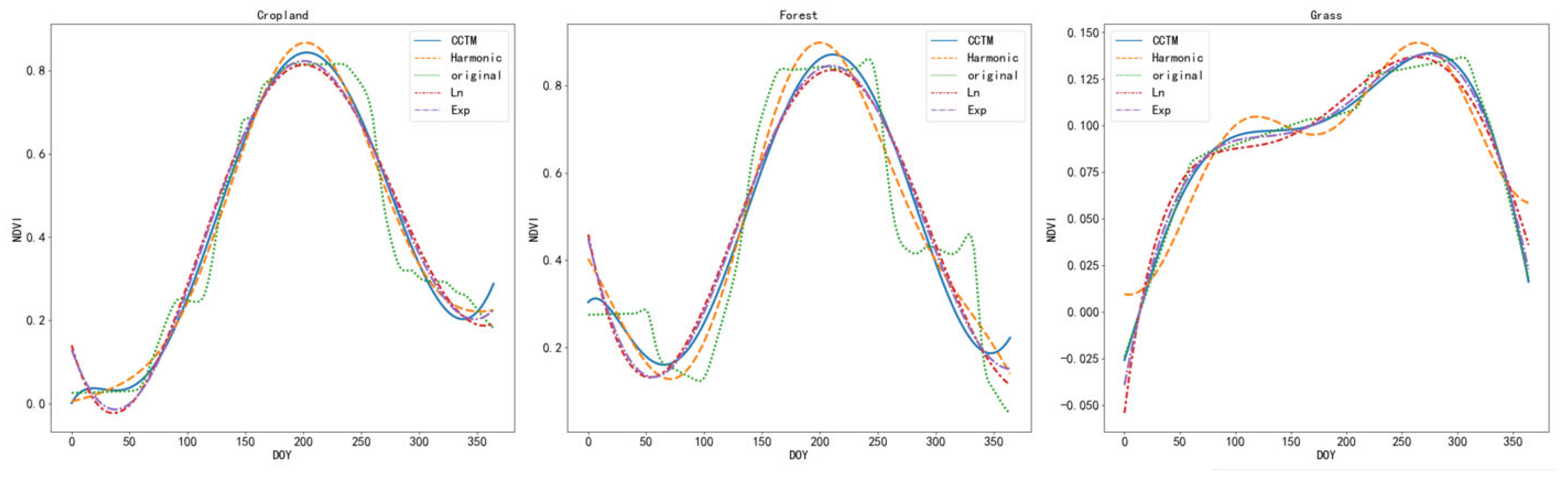
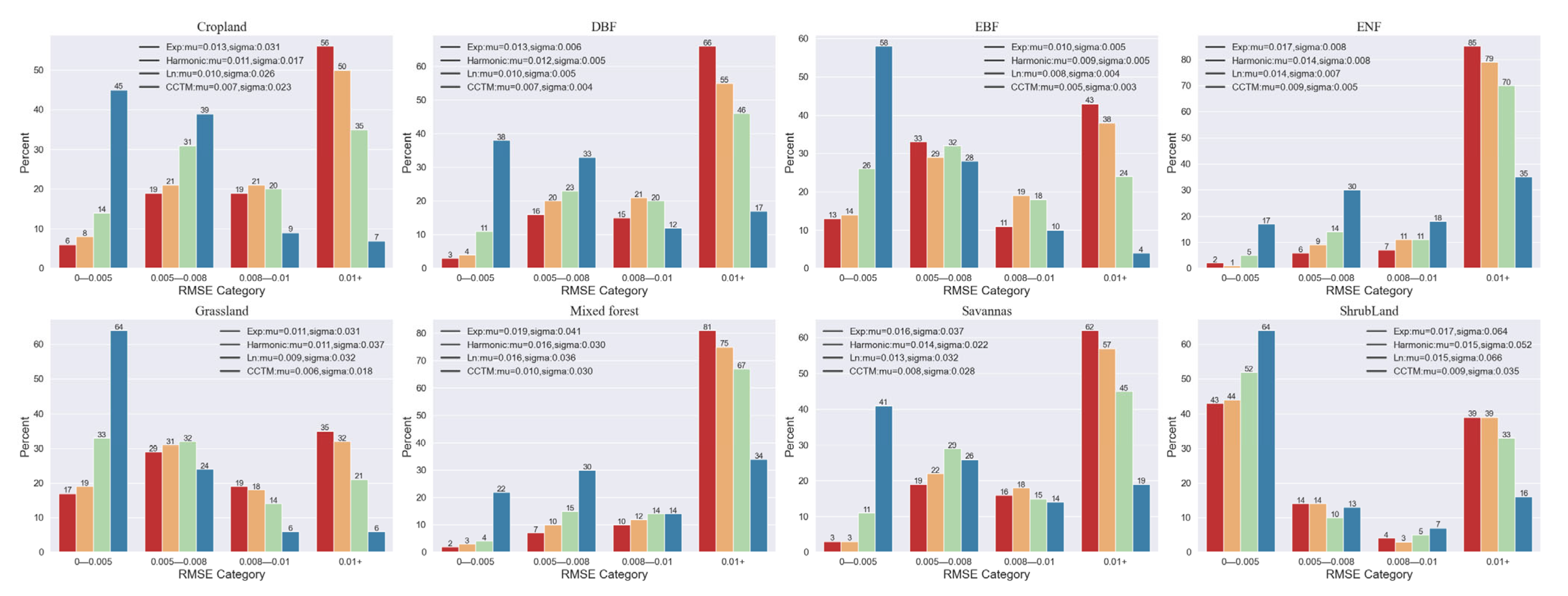
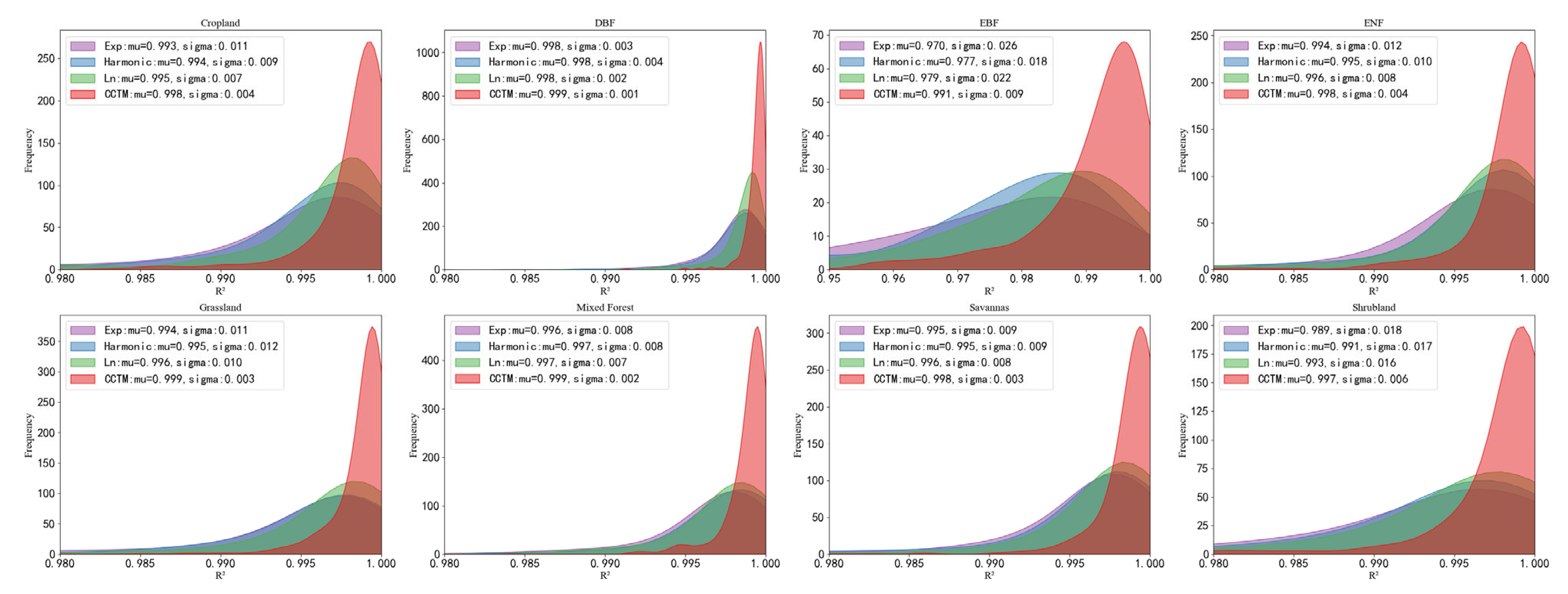
3.1. Comparison of Yearly Timeseries Pattern

The RMSE probability distribution plots in Figure 5 and the R² probability distribution plots in Figure 6 show that the Harmonic model has the strongest fitting ability for the yearly time series. More than 95%R² values and RMSE values are separately larger than 0.90 and less than 0.01 for the Harmonic model and the CCTM model. The CCTM model is slightly inferior to the Harmonic model in fitting accuracy, and the Exp model and the Ln models have shown nearly the same fitting ability. The average statistical result of R² and RMSE has shown that the Harmonic model has the best fitting accuracy, which has minimal differences from the original time series.

In addition, Figure 7 shows some of the fitting curves of different models in yearly time series patterns. The four models have some differences in the fitting effects. Although the Harmonic model and the CCTM model have nearly the same fitting effects, the Harmonic model has shown more time-series symmetrical characteristics than the CCTM model. The annual time series contains more periodic variation characteristics than the seasonal time series, and to comprehensively assess the fitting effects of the four models, the seasonal segment time-series pattern will also be compared among the four function fitting models.

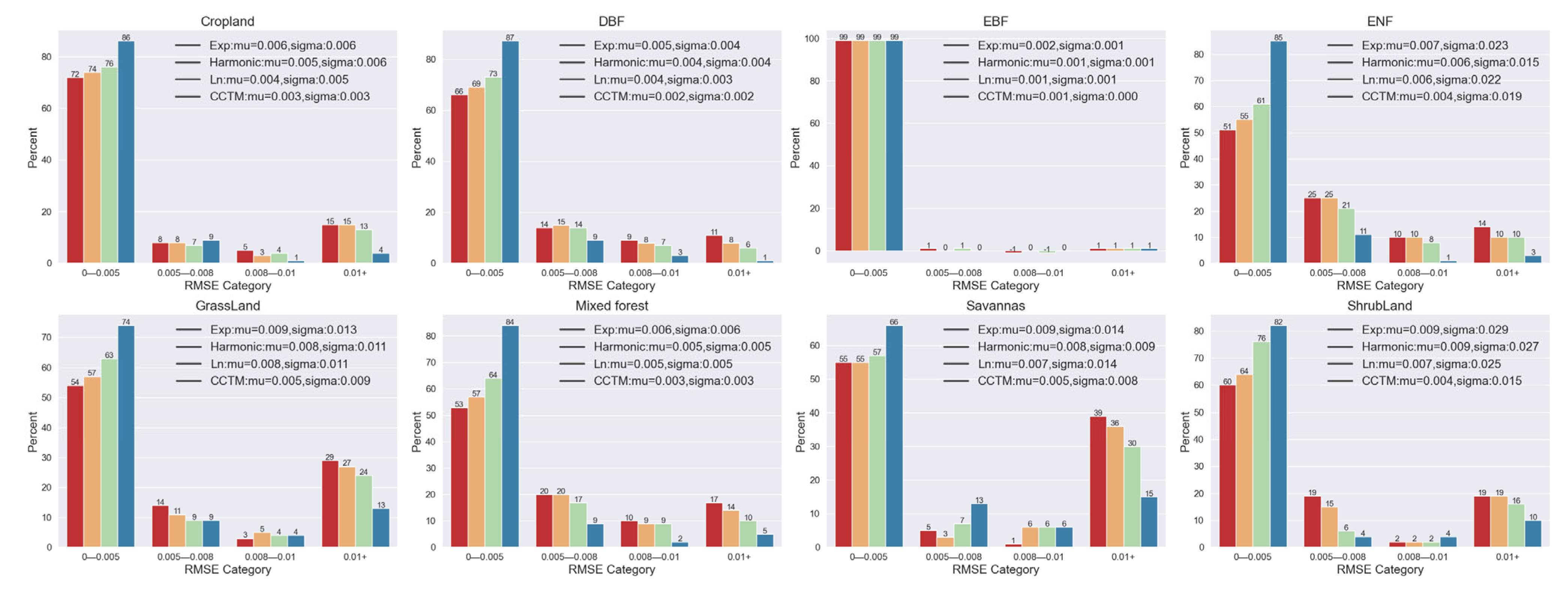
3.2. Reconstruction with Seasonal Segment Time-Series Fitting

3.2.1. Smoothing Process

Before the smoothing process of the SG filter, the gap-filled time series are extracted, and R² and RMSE between the gap-filled time series and smoothing processed time series are calculated. The final statistical results are shown in

Table 2. Statistics of the percentages of sampling points in the threshold range after smoothing.

Data type	GPP
land cover	Grassland	Cropland	DBF	EBF	ENF	MF	Savannas	Shrubland
R2 (>0.9)	99	97	100	93	100	100	99	96
RMSE (<5)	99	99	93	64	97	97	97	100
num_points	985	985	490	485	480	490	470	980
Data type	NDVI
landcover	Grassland	Cropland	DBF	EBF	ENF	MF	Savannas	Shrubland
R2 (>0.9)	95	90	100	33	94	98	94	86
RMSE (>0.01)	96	99	100	99	100	100	100	79
num_points	945	842	481	202	415	470	446	977
Data type	LAI
landcover	Grassland	Cropland	DBF	EBF	ENF	MF	Savannas	Shrubland
R2 (>0.9)	98	97	97	93	98	98	97	97
RMSE (<0.5)	100	100	91	70	94	92	98	100
num_points	979	831	490	490	480	490	485	923
Data type	MSR
landcover	Grassland	Cropland	DBF	EBF	ENF	MF	Savannas	Shrubland
R2 (>0.9)	91	96	99	94	98	99	97	67
RMSE (<0.035)	91	97	99	99	99	98	92	93
num_points	817	736	440	142	374	395	382	730

.

Before and after smoothing, nearly 95% of GPP time series data of all land cover types except EBF have smoothing RMSEs <5 g C m⁻². Almost 95% of LAI time series data of all land covers except EBF have a smoothing RMSE <5. The GPP and LAI time series data for forests, such as EBF, ENF, DBF, and MF, have relatively high RMSEs than those for grassland, cropland, savanna, and shrubland. However, the time series values of the forest types are higher than those of other land cover types, including cropland, grassland, savanna, and shrubland.

The R² result of the GPP and LAI smoothing process shows that: (1) except for cropland, EBF, and shrubland, nearly 90% of GPP time series points have R²-values >0.90. The EBF time series points have lost more original characteristics (about 30% LAI time series points have RMSE >0.5 and >30% GPP time series points have RMSE >5) than other land cover types (>90% LAI time series points have RMSE <0.5 and >95% GPP time series point have RMSE <5); (2) nearly 85% of LAI time series points of all land covers except EBF have R²-values >0.90. The smoothing processes applied to GPP and LAI time series maintained the original time series characteristics.

For the NDVI data, the smoothing process was used to reduce noise. Nearly all of the data except for shrubland have RMSEs > 0.01, and almost 95% of data except that of EBF have R²-values >0.9.

For reflectance data, more than 90% of time series points have RMSEs <0.035, and more than 90% of land cover types except shrubland have R²-values >0.9. The data for forest types, including the ENF, DBF, and MF, have higher R²-values than other land covers. In addition, the reflectance data of land cover types except shrubland have lower RMSEs and higher R²-values. This can, to some extent, indicate that the smoothing process reduces noise in the time series data and maintains its original long-term trend.

3.2.2. Reconstruction with Smoothing Process by Seasonal Segment Fitting

In this section, the time series after gap-filled and SG filter smoothing processes was defined to be the original time series, and the processed time series was the fitted time series by the four reconstruction models. The R² and RMSE values between the original and processed time series are calculated in

Table 3. Reconstruction results after smoothing.

Data Type	Models	Ln		Harmonic		Exp		CCTM		Num Points
GPP	landcover	R2 (>0.98)	RMSE (<2)	R2 (>0.98)	RMSE (<2)	R2 (>0.98)	RMSE (<2)	R2 (>0.98)	RMSE (<2)
	Grassland	83	98	96	97	84	95	99	100	995
	Cropland	64	92	85	86	65	79	94	98	990
	DBF	87	89	97	66	90	65	88	99	500
	EBF	28	41	65	28	29	18	85	81	485
	ENF	97	97	99	72	97	77	100	100	500
	MF	95	94	99	62	95	70	100	99	500
	Savannas	78	92	94	82	79	80	98	99	500
	Shrubland	79	100	92	99	80	100	98	100	990
LAI	landcover	R2 (>0.9)	RMSE (<0.5)	R2 (>0.9)	RMSE (<0.5)	R2 (>0.9)	RMSE (<0.5)	R2 (>0.9)	RMSE (<0.5)
	Grassland	95	99	99	100	96	99	97	100	934
	Cropland	86	98	98	99	89	98	92	99	880
	DBF	96	84	99	95	97	86	99	91	480
	EBF	61	34	91	57	67	31	75	48	438
	ENF	88	85	99	93	91	84	93	89	482
	MF	91	83	99	94	94	83	96	89	493
	Savannas	90	97	98	97	93	96	94	97	470
	Shrubland	92	100	98	100	93	100	96	100	976
NDVI	landcover	R2 (>0.995)	RMSE (<0.02)	R2 (>0.995)	RMSE (<0.02)	R2 (>0.995)	RMSE (<0.02)	R2 (>0.995)	RMSE (<0.02)
	Grassland	65	97	34	97	29	96	98	98	956
	Cropland	55	98	28	96	21	94	96	99	987
	DBF	90	94	55	93	49	91	100	99	491
	EBF	6	99	0	97	0	95	59	100	204
	ENF	61	85	31	88	25	75	95	96	421
	MF	76	84	43	89	35	76	98	95	475
	Savannas	75	92	37	88	30	83	98	98	456
	Shrubland	57	91	21	85	15	84	94	94	987
MSR	landcover	R2 (>0.995)	RMSE (<0.01)	R2 (>0.995)	RMSE (<0.01)	R2 (>0.995)	RMSE (<0.01)	R2 (>0.995)	RMSE (<0.01)
	Grassland	19	76	39	73	18	71	58	87	827
	Cropland	9	87	30	85	8	84	54	96	678
	DBF	27	94	54	92	27	89	77	99	447
	EBF	1	99	8	99	1	99	31	99	142
	ENF	27	90	66	90	28	86	85	97	377
	MF	32	90	67	86	36	83	81	95	396
	Savannas	23	70	64	97	27	61	74	85	827
	Shrubland	12	83	23	81	11	81	46	90	678

.

For the NDVI data, the CCTM model has a lower RMSE compared to other models (Figure 8). More than 95% of the time series points of all the land cover types except EBF have fitting R²-values >0.995, and <5% of all the time series points except shrubland type have a fitting RMSE >0.02 (Figure 9). However, for Exp and Harmonic models, more than 50% of time series points of all the land cover types have a fitting RMSE higher than 0.02. The reconstruction effect of the Ln model is not as good as the CCTM model (especially for the EBF land cover type), but it is significantly better than other models. The CCTM model generally shows considerably better performance than other models for the NDVI time series reconstruction.

For the GPP dataset (Table 3), more than 95% of the time series points of land cover types except EBF have fitting R²-values >0.98, and more than 95% of time series points of all the land cover types have fitting RMSEs <0.02 g C m⁻² using the CCTM model. The CCTM model is significantly better than other models, especially for the GPP time series of shrubland, savanna, grassland, cropland, and EBF. For other forest types, except for EBF, there are smaller differences among the four models. Overall, the CCTM model performs well for the GPP time series reconstruction for all land cover types.

For the LAI dataset (Table 3), the harmonic model shows the best reconstruction performance, with the CCTM model being slightly inferior. Except for the EBF land cover type, nearly 90% of time series points have fitting R²-values >0.9, which indicates that the CCTM model also has a great trend-preserving ability. For different land cover types, the reconstruction RMSEs are relatively inconsistent, and the forest types have larger RMSEs than non-forest types such as savanna, shrubland, and cropland. Due to the relatively low RMSE and high R²-values, the CCTM model is suitable for LAI time series reconstruction.

For the reflectance dataset, the reconstruction result after smoothing achieved high R²-values (nearly 100% of time series points have R²-values >0.9 by any of the models)(Figure 10). The CCTM model has the best reconstruction effect among the four models, and nearly all the time series points have R²-values >0.95(Figure 11). In addition, the CCTM also gained the lowest RMSE, about 90% of time series points of all land cover types have RMSE <0.01.

4. Discussion

The discussion section consists of three parts: (1) the major advantages and limitations, the reasons for high accuracy reconstruction results and the limitations of the new method are discussed in this part; (2) the potential applications; and (3) the time series functionalization and compression, the compression patterns and choices are discussed in this section.

4.1. Advantages and Limitations

In this paper, the fitting abilities of the four function fitting models are compared in the two time series patterns—the yearly time series pattern and the seasonal time series pattern. Different results exist in the two different patterns. For the yearly time series pattern, the Harmonic model shows the best fitting accuracy, and the CCTM model is slightly inferior to the Harmonic model. Most of the cropland, forest, and grassland NDVI time series have obvious seasonal time-series variation characteristics [48,49,50], and the Harmonic model has the most symmetrical fitting functions among the four function fitting models [51], so the Harmonic model has shown the best fitting accuracy among the four models.

For the seasonal time series pattern, the four function fitting models have all shown higher fitting accuracy than the models in the yearly time series pattern. Obviously, the seasonal pattern is a kind of segment fitting technique, and therefore the higher fitting accuracies were obtained in this pattern. The CCTM model has shown the highest fitting accuracy in this pattern. The CCTM model is designed according to the type of time series variation rates. It is a more comprehensive function fitting model than the Harmonic model. When it comes to time series with fewer periodic variations, such as the time series in one season, the CCTM model shows better fitting ability than the Harmonic model.

The higher accuracy of the CCTM model also shows that the CCTM model has a stronger comprehensive function fitting ability than the Harmonic model for the asymmetric time-series variations induced by vegetation growth, natural disasters, etc. From the meaning of the second derivative mathematical function, the CCTM model has more comprehensive representation techniques. Therefore, the CCTM model can be more accurate than the Harmonic model for the continuous-time series reconstruction.

The seasonal segment fitting results show that there are differences among different vegetation types. Obviously, different vegetation types mean different seasonal variation cycles and ranges of time series values, which lead to different fitting effects among different function fitting models. For the EBF vegetation type, the periodic variation characteristic is not significant in the yearly NDVI time series, and the Harmonic model and the CCTM model showed the largest differences.

However, the CCTM model has more complex function fitting structures than the Harmonic model. If there is no requirement for high-precision reconstruction results or model interpretability, the CCTM model is not suggested.

4.2. Potential Applications

Due to the high precision reconstruction effect, the CCTM model may also be applied to land surface phenology detection and monitoring, seasonal characteristics extraction, and trend analysis. For seasonal characteristic extraction, the CCTM model is specially designed to decompose the seasonal characteristics into four change parts and effectively extract the seasonal variation characteristics. For the trend analysis, because the CCTM model can decompose the time series into different variation types, the CCTM model can analyze trends of different variation types. The phenology extraction demands extracting the time series statistical features to obtain different transition states [52]. The CCTM model can represent the time series practically with high accuracy, improving the efficiency and accuracy of phenological extraction.

4.3. Time Series Functionalization and Compression

The CCTM model also provides a solution to minimize time series storage, one-year time series can be precisely characterized with only 24 coefficients in the seasonal time series pattern. The 24 coefficients can replace the original huge dataset as the new input, conducive to analyzing and applying extensive time-series data. Because extracting statistical features with a function is easier than extracting from actual time series, the functionalization for the time series can also optimize the extraction efficiency of statistical characteristics.

In addition, the coefficients have mathematical meanings, and the coefficients of different variation types represent the weights of different variations. More research is needed to explore the correlation of the coefficients with different variation types.

The CCTM model can also be applied to time series image compression. The daily time series have 365 or 366 bands, the 4-day time series dataset has approximately 90 bands, and the 8-day time series dataset has about 46 bands. All these time series can be stored in only 24 bands in the seasonal time series pattern, with each seasonal time series being fitted by the CCTM model which has 6 coefficients. Therefore the 4-day time series can approximately reach the compression ratio of 3.75, the 8-day time series dataset can approximately achieve the compression ratio of 1.91, and the daily time series dataset can approximately achieve the compression ratio of 15.

The DBF land cover type’s daily reflectance dataset and 8-day NDVI dataset have been selected to evaluate the compression effects. The CCTM model separately compresses these two datasets with 24 coefficients in seasonal time series pattern and 6 coefficients in yearly time series pattern.

The compression of the CCTM model has two patterns. The seasonal time series compression pattern which has 24 coefficients is to divide the yearly time series into four seasons. The yearly time series compression pattern which has 6 coefficients is to directly fit the yearly time series by using the CCTM model.

By using the above compression patterns, the storage before or after compression is compared and the R² between the original time series and compressed time series is calculated (

Table 4. The time series compression evaluation in two compression patterns.

Dataset	8-Day Time Series NDVI		Daily Time Series Reflectance
Compression pattern	seasonal	yearly	seasonal
Coefficient number	24	6	24
Original storage (MB)	20.63	21	163.7
Compressed storage (MB)	10.7	2.7	10.7
R2	0.99	1	0.97

). The original NDVI compression image has 383 rows, 307 columns, and 46 bands. Every pixel value is stored with a 32-bit integer, so the total image size is 20.63 MB. Similarly, the original consistent reflectance image has 365 bands, so the total image size is 163.7 MB. For the seasonal compression pattern, when applying the CCTM model to these datasets, the storage of the compressed time-series dataset for both NDVI and reflectance time series is only 10.7 MB, which is 52% of the original 8-day NDVI dataset and 6.5% of the original daily reflectance dataset.

For the yearly time series compression pattern, the final compressed NDVI and reflectance time series can be stored with only 2.69 MB, which is 13% of the original 8-day NDVI dataset and 1.6% of the original daily reflectance dataset. The number of compression coefficients should be chosen using the actual data precision when selecting the compression method.

The CCTM model is flexible on the number of the coefficients; a whole year time series can be compressed with 6 and 24 parameters. Remote sensing image compression has its standards, and the specified compression methods using the CCTM model need further research.

Due to the seasonal segment time series fitting technique, the CCTM model can achieve higher accuracy in the seasonal time series pattern than that in the yearly time series pattern, but the compression in the seasonal time series pattern needs more storage space than the compression in the yearly time series pattern. The compression pattern should be decided by the trade-off between compression ratio and compression accuracy. Only when the yearly time series compression pattern can not meet the accuracy requirement, the seasonal time series compression pattern should be adopted.

5. Conclusions

The essence of remote sensing time series reconstruction is to repair missing values by exploring and using relevant time series data. Traditional time series reconstruction methods commonly have over-smoothing and under-fitting deficiencies, and traditional reconstruction function-based models are too simple to reflect complex time series variations. Certainly, a complex model with many more parameters definitely fits data better than a simple model, but simply increasing the number of parameters is not effective. The CCTM model with 6 parameters is constructed based on the second-order derivative theorem and this is why its reconstruction precision is higher than the Harmonic model with 8 parameters. In general, the CCTM model can comprehensively reflect the complex characteristics of time series variation and embody seasonal characteristics.

Compared to the Exp, Ln, and harmonic models, the CCTM model has lower fitting errors. In the reconstruction of GPP and MSR time series with a smoothing process, >95% of time series points (except the EBF type) had R²-values >0.9 and RMSEs < 2 g C m⁻² and 0.025, respectively by using the CCTM model. For NDVI reconstruction after smoothing, >95% of time series points had R²-values >0.9 and RMSEs < 0.01 (except for the ENF and MF types) using the CCTM model. The CCTM model had the fewest extreme fitting errors but also has its limitations. Because the TP and LST time-series datasets contain too many frequent fluctuations, none of the models is suitable for their reconstruction.

Developing high-precision models can improve the precision of time series reconstruction and be beneficial in obtaining accurate knowledge of the variations in the time series dataset. Besides, the CCTM model is supposed to be applied to time series change detection, trend analysis, extraction of phenology and seasonal characteristics, time-series image compression, and land cover classification.

References

1. Ehrlich, D.; Estes, J.E.; Singh, A. Applications of NOAA-AVHRR 1 km data for environmental monitoring. Int. J. Remote Sens. 1994, 15, 145–161. [Google Scholar] [CrossRef]
2. Schepaschenko, D.; Chave, J.; Phillips, O.L.; Lewis, S.L.; Davies, S.J.; Réjou-Méchain, M.; Sist, P.; Scipal, K.; Perger, C.; Herault, B.; et al. The Forest Observation System, building a global reference dataset for remote sensing of forest biomass. Sci. Data 2019, 6, 198. [Google Scholar] [CrossRef] [PubMed] [Green Version]
3. Barnes, W.; Xiong, X.; Salomonson, V. Status of terra MODIS and aqua modis. Adv. Space Res. 2003, 32, 2099–2106. [Google Scholar] [CrossRef]
4. Irons, J.R.; Dwyer, J.; Barsi, J.A. The next Landsat satellite: The Landsat Data Continuity Mission. Remote Sens. Environ. 2012, 122, 11–21. [Google Scholar] [CrossRef] [Green Version]
5. Kuenzer, C.; Ottinger, M.; Wegmann, M.; Guo, H.; Wang, C.; Zhang, J.; Dech, S.; Wikelski, M. Earth observation satellite sensors for biodiversity monitoring: Potentials and bottlenecks. Int. J. Remote Sens. 2014, 35, 6599–6647. [Google Scholar] [CrossRef] [Green Version]
6. Kuenzer, C.; Dech, S.; Wagner, W. Remote sensing time series revealing land surface dynamics: Status quo and the pathway ahead. In Remote Sensing Time Series; Springer: Berlin/Heidelberg, Germany, 2015; pp. 1–24. [Google Scholar]
7. Liang, S.; Zhao, X.; Liu, S.; Yuan, W.; Cheng, X.; Xiao, Z.; Zhang, X.; Liu, Q.; Cheng, J.; Tang, H.; et al. A long-term Global LAnd Surface Satellite (GLASS) data-set for environmental studies. Int. J. Digit. Earth 2013, 6, 5–33. [Google Scholar] [CrossRef]
8. Tuia, D.; Ratle, F.; Pacifici, F.; Kanevski, M.; Emery, W. Active Learning Methods for Remote Sensing Image Classification. IEEE Trans. Geosci. Remote Sens. 2009, 47, 2218–2232. [Google Scholar] [CrossRef]
9. Zhu, Z.; Woodcock, C.E.; Holden, C.; Yang, Z. Generating synthetic Landsat images based on all available Landsat data: Predicting Landsat surface reflectance at any given time. Remote Sens. Environ. 2015, 162, 67–83. [Google Scholar] [CrossRef]
10. Shen, H.; Li, X.; Cheng, Q.; Zeng, C.; Yang, G.; Li, H.; Zhang, L. Missing Information Reconstruction of Remote Sensing Data: A Technical Review. IEEE Geosci. Remote Sens. Mag. 2015, 3, 61–85. [Google Scholar] [CrossRef]
11. Tian, H.; Wang, Y.; Chen, T.; Zhang, L.; Qin, Y. Early-Season Mapping of Winter Crops Using Sentinel-2 Optical Imagery. Remote Sens. 2021, 13, 3822. [Google Scholar] [CrossRef]
12. Tian, H.; Qin, Y.; Niu, Z.; Wang, L.; Ge, S. Summer Maize Mapping by Compositing Time Series Sentinel-1A Imagery Based on Crop Growth Cycles. J. Indian Soc. Remote Sens. 2021, 49, 2863–2874. [Google Scholar] [CrossRef]
13. Tian, H.; Chen, T.; Li, Q.; Mei, Q.; Wang, S.; Yang, M.; Wang, Y.; Qin, Y. A Novel Spectral Index for Automatic Canola Mapping by Using Sentinel-2 Imagery. Remote Sens. 2022, 14, 1113. [Google Scholar] [CrossRef]
14. Li, S.; Xu, L.; Jing, Y.; Yin, H.; Li, X.; Guan, X. High-quality vegetation index product generation: A review of NDVI time series reconstruction techniques. Int. J. Appl. Earth Obs. Geoinf. 2021, 105, 102640. [Google Scholar] [CrossRef]
15. Holben, B.N. Characteristics of maximum-value composite images from temporal AVHRR data. Int. J. Remote Sens. 1986, 7, 1417–1434. [Google Scholar] [CrossRef]
16. Roy, D.P. Investigation of the maximum Normalized Difference Vegetation Index (NDVI) and the maximum surface temperature (Ts) AVHRR compositing procedures for the extraction of NDVI and Ts over forest. Int. J. Remote Sens. 1997, 18, 2383–2401. [Google Scholar] [CrossRef]
17. Taddei, R. Maximum Value Interpolated (MVI): A Maximum Value Composite method improvement in vegetation index profiles analysis. Int. J. Remote Sens. 1997, 18, 2365–2370. [Google Scholar] [CrossRef]
18. Julien, Y.; Sobrino, J.A. Comparison of cloud-reconstruction methods for time series of composite NDVI data. Remote Sens. Environ. 2010, 114, 618–625. [Google Scholar] [CrossRef]
19. Wenwen, C.; Jinling, S.; Jindi, W.; Zhiqiang, X. High spatial-and temporal-resolution NDVI produced by the assimilation of MODIS and HJ-1 data. Can. J. Remote Sens. 2011, 37, 327–612. [Google Scholar] [CrossRef]
20. Gu, J.; Li, X.; Huang, C.; Okin, G. A simplified data assimilation method for reconstructing time-series MODIS NDVI data. Adv. Space Res. 2009, 44, 501–509. [Google Scholar] [CrossRef]
21. Gu, J.; Li, X.; Huang, C. Spatio-Temporal Reconstruction of MODIS NDVI Data Sets Based on Data Assimilation Methods. In Proceedings of the 8th International Symposium on Spatial Accuracy Assessment in Natural Resources and Environmental Sciences, Shanghai, China, 25–27 June 2008; pp. 242–247. [Google Scholar]
22. Lange, M.; DeChant, B.; Rebmann, C.; Vohland, M.; Cuntz, M.; Doktor, D. Validating MODIS and Sentinel-2 NDVI Products at a Temperate Deciduous Forest Site Using Two Independent Ground-Based Sensors. Sensors 2017, 17, 1855. [Google Scholar] [CrossRef] [Green Version]
23. Viovy, N.; Arino, O.; Belward, A.S. The Best Index Slope Extraction ( BISE): A method for reducing noise in NDVI time-series. Int. J. Remote Sens. 1992, 13, 1585–1590. [Google Scholar] [CrossRef]
24. Liu, R.; Shang, R.; Liu, Y.; Lu, X. Global evaluation of gap-filling approaches for seasonal NDVI with considering vegetation growth trajectory, protection of key point, noise resistance and curve stability. Remote Sens. Environ. 2016, 189, 164–179. [Google Scholar] [CrossRef] [Green Version]
25. Lovell, J.L.; Graetz, R.D. Filtering pathfinder AVHRR land NDVI data for Australia. Int. J. Remote Sens. 2001, 22, 2649–2654. [Google Scholar] [CrossRef]
26. Chen, J.; Jönsson, P.; Tamura, M.; Gu, Z.; Matsushita, B.; Eklundh, L. A simple method for reconstructing a high-quality NDVI time-series data set based on the Savitzky–Golay filter. Remote Sens. Environ. 2004, 91, 332–344. [Google Scholar] [CrossRef]
27. Chen, Y.; Cao, R.; Chen, J.; Liu, L.; Matsushita, B. A practical approach to reconstruct high-quality Landsat NDVI time-series data by gap filling and the Savitzky–Golay filter. ISPRS J. Photogramm. Remote Sens. 2021, 180, 174–190. [Google Scholar] [CrossRef]
28. Zhao, A.-X.; Tang, X.-J.; Zhang, Z.-H.; Liu, J.-H. The parameters optimization selection of Savitzky-Golay filter and its application in smoothing pretreatment for FTIR spectra. In Proceedings of the 2014 9th IEEE Conference on Industrial Electronics and Applications, Hangzhou, China, 9–11 June 2014; pp. 516–521. [Google Scholar]
29. Luo, J.; Ying, K.; Bai, J. Savitzky–Golay smoothing and differentiation filter for even number data. Signal Process. 2005, 85, 1429–1434. [Google Scholar] [CrossRef]
30. Jönsson, P.; Eklundh, L. Seasonality extraction by function fitting to time-series of satellite sensor data. IEEE Trans. Geosci. Remote Sens. 2002, 40, 1824–1832. [Google Scholar] [CrossRef]
31. Lu, X.; Liu, R.; Liu, J.; Liang, S. Removal of Noise by Wavelet Method to Generate High Quality Temporal Data of Terrestrial MODIS Products. Photogramm. Eng. Remote Sens. 2007, 73, 1129–1139. [Google Scholar] [CrossRef] [Green Version]
32. Beck, P.S.; Atzberger, C.; Høgda, K.A.; Johansen, B.; Skidmore, A. Improved monitoring of vegetation dynamics at very high latitudes: A new method using MODIS NDVI. Remote Sens. Environ. 2006, 100, 321–334. [Google Scholar] [CrossRef]
33. Sellers, P.J.; Tucker, C.J.; Collatz, G.J.; Los, S.O.; Justice, C.O.; Dazlich, D.A.; Randall, D.A. A Global 1-Degrees by 1-Degrees Ndvi Data Set for Climate Studies. The Generation of Global Fields of Terrestrial Biophysical Parameters from the Ndvi (Vol 15, Pg 3519, 1995). Int. J. Remote Sens. 1995, 16, 1571. [Google Scholar]
34. Chen, J.; Deng, F.; Chen, M. Locally adjusted cubic-spline capping for reconstructing seasonal trajectories of a satellite-derived surface parameter. IEEE Trans. Geosci. Remote Sens. 2006, 44, 2230–2238. [Google Scholar] [CrossRef]
35. Yang, G.; Shen, H.; Zhang, L.; He, Z.; Li, X. A Moving Weighted Harmonic Analysis Method for Reconstructing High-Quality SPOT VEGETATION NDVI Time-Series Data. IEEE Trans. Geosci. Remote Sens. 2015, 53, 6008–6021. [Google Scholar] [CrossRef]
36. Roerink, G.J.; Menenti, M.; Verhoef, W. Reconstructing cloudfree NDVI composites using Fourier analysis of time series. Int. J. Remote Sens. 2000, 21, 1911–1917. [Google Scholar] [CrossRef]
37. Zhou, J.; Jia, L.; Menenti, M.; Liu, X. Optimal Estimate of Global Biome—Specific Parameter Settings to Reconstruct NDVI Time Series with the Harmonic ANalysis of Time Series (HANTS) Method. Remote Sens. 2021, 13, 4251. [Google Scholar] [CrossRef]
38. Zhou, J.; Jia, L.; van Hoek, M.; Menenti, M.; Lu, J.; Hu, G. An optimization of parameter settings in HANTS for global NDVI time series reconstruction. In Proceedings of the 2016 IEEE International Geoscience and Remote Sensing Symposium (IGARSS), Beijing, China, 10–15 July 2016; pp. 3422–3425. [Google Scholar]
39. Zhou, J.; Jia, L.; Menenti, M. Reconstruction of global MODIS NDVI time series: Performance of Harmonic ANalysis of Time Series (HANTS). Remote Sens. Environ. 2015, 163, 217–228. [Google Scholar] [CrossRef]
40. Xu, L.; Li, B.; Yuan, Y.; Gao, X.; Zhang, T. A Temporal-Spatial Iteration Method to Reconstruct NDVI Time Series Datasets. Remote Sens. 2015, 7, 8906–8924. [Google Scholar] [CrossRef] [Green Version]
41. Cao, R.; Chen, Y.; Shen, M.; Chen, J.; Zhou, J.; Wang, C.; Yang, W. A simple method to improve the quality of NDVI time-series data by integrating spatiotemporal information with the Savitzky-Golay filter. Remote Sens. Environ. 2018, 217, 244–257. [Google Scholar] [CrossRef]
42. Friedl, M.A.; Sulla-Menashe, D.; Tan, B.; Schneider, A.; Ramankutty, N.; Sibley, A.; Huang, X. MODIS Collection 5 global land cover: Algorithm refinements and characterization of new datasets. Remote Sens. Environ. 2010, 114, 168–182. [Google Scholar] [CrossRef]
43. Ma, M.; Veroustraete, F. Reconstructing pathfinder AVHRR land NDVI time-series data for the Northwest of China. Adv. Space Res. 2006, 37, 835–840. [Google Scholar] [CrossRef]
44. Jönsson, P.; Eklundh, L. TIMESAT—A program for analyzing time-series of satellite sensor data. Comput. Geosci. 2004, 30, 833–845. [Google Scholar] [CrossRef] [Green Version]
45. Madden, H.H. Comments on the Savitzky-Golay convolution method for least-squares-fit smoothing and differentiation of digital data. Anal. Chem. 1978, 50, 1383–1386. [Google Scholar] [CrossRef]
46. Zhu, Z.; Woodcock, C.E. Continuous change detection and classification of land cover using all available Landsat data. Remote Sens. Environ. 2014, 144, 152–171. [Google Scholar] [CrossRef] [Green Version]
47. Zhu, Z.; Woodcock, C.E.; Olofsson, P. Continuous monitoring of forest disturbance using all available Landsat imagery. Remote Sens. Environ. 2012, 122, 75–91. [Google Scholar] [CrossRef]
48. Liu, J.; Liu, M.; Tian, H.; Zhuang, D.; Zhang, Z.; Zhang, W.; Tang, X.; Deng, X. Spatial and temporal patterns of China’s cropland during 1990–2000: An analysis based on Landsat TM data. Remote Sens. Environ. 2005, 98, 442–456. [Google Scholar] [CrossRef]
49. Lausch, A.; Erasmi, S.; King, D.J.; Magdon, P.; Heurich, M. Understanding Forest Health with Remote Sensing -Part I—A Review of Spectral Traits, Processes and Remote-Sensing Characteristics. Remote Sens. 2016, 8, 1029. [Google Scholar] [CrossRef] [Green Version]
50. Liu, Y.; Hill, M.J.; Zhang, X.; Wang, Z.; Richardson, A.D.; Hufkens, K.; Filippa, G.; Baldocchi, D.D.; Ma, S.; Verfaillie, J.; et al. Using data from Landsat, MODIS, VIIRS and PhenoCams to monitor the phenology of California oak/grass savanna and open grassland across spatial scales. Agric. For. Meteorol. 2017, 237–238, 311–325. [Google Scholar] [CrossRef]
51. Katznelson, Y. An Introduction to Harmonic Analysis; Cambridge University Press: Cambridge, UK, 2004. [Google Scholar]
52. Zhang, X.; Friedl, M.A.; Schaaf, C.B.; Strahler, A.H.; Hodges, J.C.F.; Gao, F.; Reed, B.C.; Huete, A. Monitoring vegetation phenology using MODIS. Remote Sens. Environ. 2003, 84, 471–475. [Google Scholar] [CrossRef]
Figure 1. Flowchart of time series reconstruction.
Remotesensing 14 02280 g001
Figure 2. Distribution of sampling points and stable land cover types. 13 kinds of stable land cover types from 2001 to 2005 are extracted from the MCD12Q1.006 product. For 9 kinds of vegetation land cover types, 100 sampling points for each of the ENF, EBF, DBF, and MF datasets and 200 sampling points for each of the shrubland, savanna, grassland, and cropland datasets are obtained.
Remotesensing 14 02280 g002
Figure 3. Gap-filling method. Solid time series points represent known time series values, and hollow time series points represent missing time series values.
Remotesensing 14 02280 g003
Figure 4. Trend-fill method.
Remotesensing 14 02280 g004
Figure 5. Fitting RMSE distribution on different land cover types among different models. The figs reflect the fitting RMSE probability density distributions of different models. The frequency is the number of time series points in a certain RMSE range, and different land cover types may have different RMSE categories.
Remotesensing 14 02280 g005
Figure 6. R2 distribution on different land cover types among different models. The figs reflect the fitting R2probability density distributions of different models. The frequency is the number of time series points in the certain R2 range, and different land cover types may have different RMSE categories.
Remotesensing 14 02280 g006
Figure 7. The fitting curves of different models with no seasons division. The figs reflect the yearly time series fitted by the CCTM, Harmonic, Exp, and Ln models.
Remotesensing 14 02280 g007
Figure 8. Reconstruction RMSE distribution of NDVI time series data with smoothing process. The frequency is the percentage of time series points in the certain RMSE range, and different landcover types may have different RMSE categories.
Remotesensing 14 02280 g008
Figure 9. R2 probability distribution of reconstructed NDVI time-series data after smoothing for different landcover types. The frequency is the number of time series points in a certain RMSE range, and different landcover types may have different RMSE categories.
Remotesensing 14 02280 g009
Figure 10. RMSE of reconstructed MSR time series data after smoothing for different landcover types. The frequency is the percentage of the certain RMSE range, and different landcover types may have different RMSE categories.
Remotesensing 14 02280 g010
Figure 11. R2 probability distribution of reconstructed MSR time series data after smoothing for different landcover types. The frequency is the number of time series points in a certain RMSE range, and different landcover types may have different RMSE categories.
Remotesensing 14 02280 g011