

Forest Height Inversion Based on Time–Frequency RVoG Model Using Single-Baseline L-Band Sublook-InSAR Data


1
School of Civil Engineer and Geomatics, Southwest Petroleum University, Chengdu 640500, China
2
National Tibetan Plateau Data Center, State Key Laboratory of Tibetan Plateau Earth System, Environment and Resources (TPESER), Institute of Tibetan Plateau Research, Chinese Academy of Sciences, Beijing 100101, China
3
School of Environment and Spatial Informatics, China University of Mining and Technology, Xuzhou 221116, China
*
Author to whom correspondence should be addressed.
Remote Sens. 2023, 15(1), 166; https://0-doi-org.brum.beds.ac.uk/10.3390/rs15010166
Submission received: 18 October 2022
/
Revised: 24 December 2022
/
Accepted: 24 December 2022
/
Published: 28 December 2022
(This article belongs to the Special Issue SAR for Forest Mapping II)
Abstract
:The interferometric synthetic aperture radar (InSAR) technique based on time–frequency (TF) analysis has great potential for mapping the forest canopy height model (CHM) at regional and global scales, as it benefits from the additional InSAR observations provided by the sublook decomposition. Meanwhile, due to the wider swath and higher spatial resolution of single-polarization data, InSAR has a higher observation efficiency in comparison with PolInSAR. However, the accuracy of the CHM inversion obtained by the TF-InSAR method is attenuated by its inaccurate coherent scattering modeling and uncertain parameter calculation. Hence, a new approach for CHM estimation based on single-baseline InSAR data and sublook decomposition is proposed in this study. With its derivation of the coherent scattering modeling based on the scattering matrix of sublook observations, a time–frequency based random volume over ground (TF-RVoG) model is proposed to describe the relationship between the sublook coherence and the forest biophysical parameters. Then, a modified three-stage method based on the TF-RVoG model is used for CHM retrieval. Finally, the two-dimensional (2-D) ambiguous error of pure volume coherence caused by residual ground scattering and temporal decorrelation is alleviated in the complex unit circle. The performance of the proposed method was tested with airborne L-band E-SAR data at the Krycklan test site in Northern Sweden. Results show that the modified three-stage method provides a root-mean-square error (RMSE) of 5.61 m using InSAR and 14.3% improvement over the PolInSAR technique with respect to the classical three-stage inversion result. An inversion accuracy of RMSE = 2.54 m is obtained when the spatial heterogeneity of CHM is considered using the proposed method, demonstrating a noticeable improvement of 32.8% compared with results from the existing method which introduces the fixed temporal decorrelation factor.
1. Introduction
A forest canopy height model (CHM) is important for the detection of forest harvesting, forest degradation, and forest fires [1]. Moreover, timely access to accurate estimates of the above-ground forest biomass would assist in studying the regional and global carbon cycle and climatic variation [2,3,4,5].
At present, ground measurement, light detection and ranging (LiDAR), and interferometric synthetic aperture radar (InSAR) have been widely applied to estimate the CHM for different forest types (boreal, temperate, and tropical forests). Due to the low efficiency and the high cost of data acquisition, it is difficult for ground measurement to meet the requirements of rapid and large-scale CHM mapping. Meanwhile, the accuracy of the measured forest CHM is limited by the density of sampling points [6]. LiDAR and InSAR, as active remote sensing techniques, have significant advantages over ground-based measurements in terms of the scope of data observation. However, the application of ground-based or airborne LiDAR is limited by the coverage of data and the exorbitant price [7,8]. In addition, the spaceborne LiDAR (e.g., ICESat [9]) is susceptible to cloud interference and has difficulty penetrating dense forests. Fortunately, InSAR has great potential for large-scale and high-accuracy CHM mapping because of the strong penetration ability of its radar wave, its independence from weather conditions, and its sensitivity to the vertical distribution of scatterers [10].
The CHM inversion methods based on the InSAR technique can be divided into three categories, which are described as follows.
(1) Traditional InSAR inversion: There are two ways to estimate the CHM from InSAR observations. On the one hand, the CHM can be extracted from the gap between the center height of the interference phase of the single-polarization InSAR and the external underlying DEM [11,12]. It is inevitable that the accuracy of the CHM estimates largely depends on the high-precision of the external underlying DEM, which is generally difficult to obtain. On the other hand, the degraded random volume over ground (RVoG) model can also be used to estimate the CHM from InSAR data, but it reduces the accuracy of the CHM.
(2) PolInSAR inversion: Polarimetric SAR interferometry (PolInSAR) is developed from InSAR by combining it with multi-polarization information. With this technique, different scatterers which are located in the vertical dimension of the same pixel can be detected, and then the CHM estimates can be obtained without using other external data [13,14,15,16]. Moreover, the multi-baseline technique developed in recent years further provides a variety of spatial observation schemes for PolInSAR to improve the accuracy of the CHM inversion [17,18,19,20]. As a result, these improved techniques can be used to avoid the underdetermined problem of unknown parameters based on a vegetation scattering model (e.g., RVoG), which makes it possible to obtain the high-precision CHM. However, the CHM inversion based on the multi-polarization data comes at the cost of reducing the observation efficiency of InSAR. This is because the PolInSAR technique usually has a smaller swath and lower spatial resolution than the single-polarization case [21].
(3) Sublook InSAR inversion: The time-frequency (TF) analysis method provides a new pathway for high-precision CHM inversion. In previous studies, the dual-polarization TF optimization method has been used to estimate the accurate interference phase of pure volume coherence and the ground phase [22], which helps to improve the accuracy of the CHM inversion. Besides, the TF optimization method has also been extended to the full-polarization case [23]. It can be seen that the TF analysis can be used as an improved method to obtain the optimal coherence. However, compared with single-polarization InSAR, the dual- and full-polarization cases will lower the observation efficiency.
In the single-polarization case, the Time-frequency and Line-fitting (TF + LF) method with a priori extinction coefficient has been proposed for the CHM inversion from the single-baseline InSAR data. It can not only solve the underdetermined problem of unknown parameters but also avoid the low observation efficiency of the PolInSAR technique [6,24]. However, the performance of this method is usually affected by three factors. The first one comes from the coherent scattering model. In the TF + LF method, the sublook coherence plays a similar role to that of the RVoG-based polarization coherence. However, an essential difference between the sublook and polarimetric observations has not been revealed in the TF + LF method, which leads to an ambiguous interpretation of the impact of the sublook observations. As for the difference, it is known that the polarization coherences are determined by the different polarization states, whereas the sublook coherences are distinguished by the path differences of the sublook SAR signals, which are caused by the varying azimuth observation angles. The second problem is referred to as the defective parameter inversion. Namely, a small amount of CHM is necessary to extract the extinction coefficient which will be used as a priori knowledge. The third problem is the impact of the pure volume coherence error. The estimated CHM is sensitive to the 2-D ambiguous error of pure volume coherence, which is induced by the joint impacts of the residual ground scattering and the temporal decorrelation and is difficult to removed in the single-baseline inversion.
Therefore, the CHM inversion method based on TF analysis has great potential to extract a high-precision CHM benefitting from the more available observations provided by the sublook decomposition and the higher observation efficiency of the single-polarization InSAR. However, the inaccurate coherent scattering modeling and parameter inversion are major problems that limit the accuracy of the CHM estimation.
According to the above methods, the information from each scatterer is collected at various incidence angles, and the sublook coherences along the azimuth carry different backscattering properties. Note that the essential reason for this is the path difference of the sublook SAR signals through the forest volume, which is important for the model-based CHM inversion from the sublook coherences, and should be further studied. As a result, the scattering matrix was reconstructed in consideration of the path differences of sublook observations in this paper. With a derivation of coherent scattering modeling based on the reconstructed scattering matrix, a more accurate sublook coherent scattering model, namely, the TF-RVoG model, is proposed for the CHM inversion from sublook InSAR data. Regarding the height of the phase center for different sublook coherences, the pure volume coherence can be obtained from the alternative sublook coherences. Hence, a single-baseline three-stage method for the TF-RVoG model was also proposed in this work. In order to obtain a higher accuracy for the CHM, the empirical relationship between (which is the distance ratio index used to describe the position of pure volume coherence in the coherence line [25]) and the extinction coefficient is used to alleviate the residual ground scattering error of the pure volume coherence. In addition, the strong correlation between the temporal decorrelation and the CHM is verified, and a random volume over ground with mutative temporal decorrelation (RVoG + MTD) model that takes into account the spatial heterogeneity of the forest CHM is proposed to remove the temporal decorrelation error. The advantages of the proposed approach are as follows:
- (1)
- It considered the path difference of sublook SAR signals and can help to provide detailed interpretation for the impact of the different sublook coherences in the sublook coherent scattering modeling;
- (2)
- It can invert the forest CHM from the single-baseline and single-polarization InSAR data without an a priori CHM, underdetermined parameter inversion, and observation efficiency reduction;
- (3)
- It can alleviate the influence of the 2-D ambiguous error of pure volume coherence by combining the empirical relationship of the and the extinction coefficient [25] with the RVoG + MTD model.
The rest of this paper is structured as follows. Section 2 introduces the principle and modeling process of the proposed TF-RVoG model, the correction of interferometric phase error of sublook coherences induced by the residual motion error (RME) [26], the three-stage CHM inversion process based on the TF-RVoG model, and the correction of 2-D ambiguous error of pure volume coherence. In Section 3, the performance of the proposed approach is tested using single-baseline L-band InSAR data acquired by the German Aerospace Center (DLR)’s airborne E-SAR system. Discussion of and conclusions about the proposed approach are presented in Section 4 and Section 5, respectively.
2. Theory and Method
2.1. Sublook Coherent Scattering Modeling
In the TF analysis, fast Fourier transform (FFT) filtering is used to split the full-resolution SAR image into several sublook images [27,28,29], and then the target can be detected using various azimuth observation angles from the different sublook SAR images. The azimuth observation angle can be expressed as a function of the Doppler frequency , the radar wavelength , and the platform velocity [30]
It is the angle between the sight line associated with a zero Doppler centroid and the random sight line, which determines the relative position of a sublook along the azimuth. Moreover, can range from to , and is the variation interval of the azimuth observation angle related to the azimuth resolution of the sublook image. As shown in Figure 1 (top), FFT filtering of the full-resolution SAR-image frequency spectra is performed in the azimuth direction to form three sublooks of equivalent resolution with a 50% overlap, which are represented as green, red, and blue dashed rectangles. Note that only the Doppler spectra of the red and blue sublooks are independent. Here, the green, red, and blue arrows in Figure 1 (bottom) denoted the azimuth observation angles which are related to the three sublooks. Since the filtered bandwidths are constant, the intervals of the observation angle are equivalent for the three sublooks.
Two sublook images and with the same and can be acquired by performing the sublook decomposition of the full-resolution master and slave images, respectively. After interferometric processing, the corresponding sublook coherence can be expressed as [24]
where 〈 〉 represents the expected value. is impacted by several decorrelation factors, such as the signal-to-noise decorrelation, the geometric decorrelation, and the temporal decorrelation, which can be reduced or absorbed by the associated correction methods [31,32,33]. On this basis, the sublook coherence is approximately equivalent to the volume decorrelation related to the backscattering properties of scatterers in forest scenes.
It is clear that the sublook coherences help to increase InSAR observations, which makes it possible to invert the CHM in the case of single-polarization InSAR. Therefore, a sublook coherent scattering model, which can be used to accurately describe the relationship between the sublook coherence and the forest biophysical parameters, must be built for the CHM inversion. However, the varying azimuth observation angles of the sublook coherences result in the path difference of the sublook signals in the forest volume, which can cause backscattering variations because of the anisotropic geometrical structures of the real forest volume. Therefore, the path impacts of the different sublook signals need to be considered and accounted for in the coherent scattering model.
Based on the above analysis, the scattering matrix can be expressed as [32]
where the superscript denotes the transpose of a given matrix, and the impacts of the different propagation paths of sublook signals can be expressed with a 2 × 2 propagation matrix which is defined as
where and are in general complex, relating to both phase shift and attenuation in the forest volume. Specifically, , , and is the free space wavenumber, which is equal to . and represent the propagation value of the horizontal polarization and vertical polarization, respectively. The expression describes the process of the sublook signals’ propagation into and then out of the medium.
After vectorization processing based on the Pauli basis, the scattering matrix can be transformed into a four-dimensional (4-D) vector expressed as
where is the differential propagation constant; , as a 4 × 4 matrix, represents the propagation matrix associated with propagation path within the medium; and sinh and cosh are hyperbolic sine and hyperbolic cosine functions, respectively. In the case of a random medium, the parameter s is equal to zero, and reduces to a multiple of the identity matrix. Furthermore, is a 4-D scattering vector that does not the propagation influence on the vegetation backscattering. Based on the reciprocity theorem for antennae, namely, the scattering vector can be simplified as a three-dimensional (3-D) vector expressed as
where is the corresponding 3 × 3 propagation matrix, and is the scattering vector which is free from the propagation influence.
According to the three-component decomposition based on the different scattering mechanisms, the scattering vector can be expressed as
where the greater complexity of scattering (higher than second order) is not considered, and the propagation matrix related to the volume scattering mechanism is approximately equivalent to an identity matrix. The subscripts 1 and 2 represent the corresponding master image and slave image, and the subscripts , , and represent the volume, surface, and dihedral scattering mechanisms, respectively. and are the corresponding 3 × 3 propagation matrices of the surface and dihedral scattering. In the same way, , , and are the scattering vectors of the volume, surface, and dihedral scattering mechanisms, respectively [32]. Moreover, the coherency matrix is formed by the 3-D coherent scattering vectors and for each end of the baseline, and is expressed as
With the combination of (7) and (8), the coherency matrices and can be decomposed into three components on the basis of the different scattering mechanisms, respectively, and are shown as
As a result, we can express the interferometric coherence of the single-polarization as
where is the projection vector related to the polarization, can be expressed as a function of the coherency matrices and and the propagation matrix based on the approximate condition . The subscript represents a kind of scattering mechanism. In this case, we can rewrite (11) based on the equivalent transformation, which is shown as [32]
where is the normalized radar cross section and represents the coherence contribution. The propagation factor related to the propagation path can be described as a function of the azimuth observation angle and used to attenuate the corresponding contribution of each scattering mechanism . Note that the sublook coherences are obtained from a pair of given full-resolution SAR images with a fixed polarimetric state. Therefore, the projection vector is constant for the different sublook coherences. As a result, the sublook interferometric coherences with different azimuth observation angles can be expressed as
In general, it is assumed that the surface and dihedral scattering mechanisms include equal coherence contributions, which is shown as
Therefore, the interferometric coherence related to a given polarimetric state can be rewritten, and is shown as
where is the ground phase associated with the underlying topography, denotes the ground-to-volume scattering ratio, which is formulated as a function of the ground- (surface and dihedral) and volume- backscattering contribution, and is shown as
In addition, represents the pure volume scattering coherence, which is modeled as a function of the forest’s biophysical parameters and the vertical wavenumber with an exponential backscattering profile, as shown in (17).
where is the CHM and is the look angle of the master track. denotes the extinction coefficient, which is used to describe the power attenuation of the SAR signals in the forest volume. is the vertical wavenumber impacted by the baseline parameters and topographic slope.
Finally, for the single-polarization InSAR data, the sublook interferometric coherence, which is related to the azimuth observation angle , can be derived from the Equations (15)–(17) and is shown as
where is expressed as a function of the azimuth observation angle . The reason is that results in the path difference of the sublook signals in the forest volume, and σ can be influenced by the azimuth observation angle in a forest volume with heterogeneous characteristics. Moreover, for the sublook coherences caused by the different azimuth observation angles, both the polarimetric state and the variation interval of the azimuth observation angle are fixed. In this case, the corresponding ground-to-volume scattering ratio and extinction coefficient can be influenced by the azimuth observation angle . As a result, Equation (18), which has a similar expression to that of the OVoG model [34], is not invertible because of the underdetermined problem of unknown parameters.
To address this problem, the change in the extinction coefficient caused by the different azimuth observation angles within the volume scattering coherence can be ignored, since the difference in azimuth observation angles leads to a significant offset of the sublook coherences along the coherence line but a relatively small change in the pure volume coherence () in the complex plane, as has been verified in several studies [6,24]. Therefore, we can rewrite the sublook coherence as
It is clear that Equation (19) shows the relationship between the sublook coherences and the forest’s biophysical parameters. According to the previous discussion, a full-resolution SAR image can be split into multiple sublook images by performing sublook decomposition, and then the corresponding sublook coherences can be acquired using interferometric processing (see Equation (2)). In this case, the number of observations made using the classical InSAR system is increased by changing the azimuth observation angle , which makes it possible to quantitatively evaluate the unknown parameters based on the Equation (19). In the complex plane, the coherence points corresponding to different sublooks can be enveloped by a polygon called the coherence region [24]. The coherence region can be fitted as a line using the Line-fitting (LF) method, as in the case of the RVoG model. In such a case, it is possible to estimate the ground phase and the forest biophysical parameters in the complex circle.
Equation (19) describes the vegetation scattering model as a two-layer structure made up of a volume layer and a ground layer. It can be called the TF-RVoG model because of the use of the TF analysis. Note that the impacts of the different azimuth observation angles on the ground-to-volume scattering ratios are described by a pair of propagation factors and , as shown in Equation (16). The reason for this is that, with the difference in propagation paths caused by the varying azimuth observation angles, the sublook SAR signals undergo different attenuation in the heterogeneous forest volume, which results in a pair of varying propagation factors and . However, for the RVoG-based polarimetric observations, the ground-to-volume scattering ratio is determined by the different , , and . This indicates a significant difference in the impacts of the sublook and polarimetric coherences.
Moreover, an ideal case is provided to study in further detail the differences in the sublook and polarimetric InSAR observations, where the forest is a homogeneous volume with the same CHM and the underlying topography is a horizontal plane, as shown in Figure 2a. In this case, the pure volume coherence is a constant because of the fixed extinction coefficient of the homogeneous forest, and we can compare the coherence loci of the sublook and polarimetric observations in the complex unit circle. For the RVoG-based polarimetric coherences, the ground-to-volume scattering ratio is changed by the normalized radar cross section for the different polarimetric states. As a result, the coherence loci of the polarimetric observations strictly follow a straight line, as shown in Figure 2b. For the sublook coherences based on the TF-RVoG model, however, the propagation factors and are invariable since the different sublook SAR signals undergo the same attenuation process in the ideal forest scene. Therefore, the corresponding coherence loci of the sublook observations present as isolated points with a constant ground-to-volume scattering ratio (Figure 2c).
2.2. RME-Induced Phase Error Correction
Due to the changes in the backscattering properties caused by the different propagation paths of the sublook SAR signals, the sublook coherences contain different interferometric phases. To accurately estimate the CHM from the sublook coherences, we must ensure that the change in the backscattering properties is the only factor leading to the interferometric phase difference of the sublook coherences. Therefore, the phase components that are induced by other factors varying with the different azimuth observation angles must be removed. For the airborne InSAR data used in this paper, the interferometric phase error caused by the residual motion error (RME) is the major influence factor [26].
With the impact of airflow turbulence, the airborne SAR sensor usually deviates from its predetermined track along the azimuth, which leads to a time-varying motion error. After interference processing, the motion error will be transformed into the error of the interferometric phase. In general, the motion error impacts of the different polarization coherences can be ignored when estimating the CHM by using the PolInSAR data. However, for the sublook InSAR coherences, a varying phase component will be induced by the different motion errors along the azimuth, which will have a negative impact on the CHM inversion. In other words, these motion errors are unabsorbable and must be removed for robust parameter estimation in the case of sublook InSAR. According to the existing studies, the motion parameters of aircraft can be record by the navigation system of the airborne SAR sensor, and most of the motion error can be removed through motion compensation processing [35,36,37]. However, there a fraction of RME will remain because of the limited precision of the current airborne navigation system.
To remove the RME-induced phase error of each sublook coherence, a parameterized model for the single-baseline case that can accurately describe the relationship between the errors of the time-varying baseline parameters and the RME-induced interferometric phase is used, and it can be expressed by Equation (20) [26]
where is the differential interferometric phase, including three phase components: the RME-induced phase , the topographic error phase caused by discrepancies between the external digital elevation model (DEM) and the real DEM, and the noise phase . Furthermore, and are the time-varying baseline parameter errors, which are related to the baseline length and the baseline tilt angle . Note that can be divided into two parts, i.e., the residual flat-earth phase and the residual topographic phase . represents the unwrapped phase of the reference point, and denotes the sum of the topographic error phase and the noise phase. Based on this model, three unknown parameters , , and can be jointly estimated using a weighted least-squares (WLS) regression approach. As a result, we can acquire the corresponding RME-induced phase error and then deduct it from each sublook interferometric phase with the same processing.
2.3. Three-Stage Inversion Method Based on the TF-RVoG Model
The proposed TF-RVoG model has a similar expression to that of the RVoG model. However, for the sublook coherences based on the TF-RVoG model, it is difficult to estimate the CHM using the classical three-stage inversion method [15] for the following two reasons. Firstly, for the RVoG-based polarimetric observations, we can acquire the ground phase from the two intersection points between the coherence line and the unit circle in the complex unit circle using the a priori order of the polarimetric coherences along the coherence line. However, there is no a priori order of the sublook coherences to use in selecting the ground phase. Secondly, a measured coherence with a zero ground scattering component, i.e., the pure volume coherence, is needed to invert the CHM from a 2-D lookup table (LUT) with the CHM and the extinction coefficient. In the polarimetric cases, the coherence of HV or PDH polarization, which includes a lower ground scattering contribution in comparison with the other polarizations, is usually selected as the pure volume coherence. However, the pure volume coherence for the sublook observations is unknown.
To address these problems, a modified three-stage method that is suitable for the TF-RVoG model is proposed for the CHM inversion, and the detailed steps are as follows.
(1) Coherence Line Fitting: Based on Equation (19), the sublook coherences are impacted by the varying ground-to-volume scattering ratios caused by the different propagation factors. Hence, the coherence loci of the sublook InSAR observations form a finite line between the coherence of the ground phase and the pure volume coherence in the complex plane. Therefore, sublook coherences with different azimuth incidence angles can be fitted to a coherence line using the total least-squares (TLS) method.
(2) Ground Phase Selection: Two intersection points between the fitted coherence line and the complex unit circle are considered as candidate ground phase points, and we need to select the correct ground phase point from these two candidates without a priori knowledge. Due to the monotonic lowering of the sublook phases with the increase in the ground-to-volume scattering ratios, a robust criterion was derived in [38] that can be used to obtain the correct ground phase point in the sublook case. The corresponding decision rule is shown as
where is the ground phase, and and are the two candidate ground phases. This criterion with a limited condition of is effective for selecting the true ground phase and is free of the a priori order of the sublook coherences.
(3) Forest CHM Retrieval: To avoid the underdetermined problem in the CHM inversion, a coherence without the ground scattering contribution (i.e., ) needs to be selected from all the observed sublook coherences. Based on the opposite relationship between the interferometric phases of the sublook coherences and the corresponding ground-to-volume scattering ratios, the phase center height of each sublook coherence can be expressed as
When the condition of is satisfied, the sublook coherence with the lowest ground scattering contribution can be acquired from the candidate sublook coherences. In this case, we can rewrite the (19) as
As a result, a pair of the corresponding solutions ) can be retrieved in the form of the 2-D LUT.
2.4. 2-D Ambiguous Error Correction of the Pure Volume Coherence
For the sublook InSAR data, the CHM can be retrieved by the modified three-stage method without a priori knowledge. However, the accuracy of the CHM inversion is impacted by two major problems, i.e., the residual ground scattering error of the pure volume coherence and the temporal decorrelation error.
(1) Residual Ground Scattering Effect: Equation (22) shows that the sublook coherence with the lowest ground scattering contribution can be selected from all the sublook coherences, and it is regarded as the pure volume coherence. In the complex unit circle, the obtained pure volume coherence is located at the end of the coherence region farther from the ground phase point , as shown in Figure 3a. However, due to the influence of the residual ground scattering error, the true pure volume coherence without considering the temporal decorrelation error should be located on a finite line between the and , as shown in Figure 3b, which causes a one-dimensional (1-D) ambiguous error of the pure volume coherence along the coherence line.
(2) Temporal Decorrelation Effect: In an airborne repeat-pass interferogram, the temporal decorrelation error caused by repeated SAR acquisitions can result in an overestimated CHM [33,38,39]. During a short time interval (about 50 min in this paper), the wind-induced motion of the scatterers in the forest volume is the major factor causing the temporal decorrelation error of the airborne InSAR system. According to the existing studies, we can assume that the temporal decorrelation error only changes the amplitudes of the sublook coherences and has no effect on their phases [40]. In this case, the true pure volume coherence will be located on the extended segment of the finite line between and the center of the circle, forming the second 1-D ambiguous error (Figure 3c).
Therefore, in the complex unit circle, a 2-D ambiguous error in the pure volume coherence is caused by the joint influence of the residual ground scattering contribution and the temporal decorrelation, which needs to be removed to obtain a high-precision CHM.
To address these problems, firstly, a geometrical index , which can interpret the relative location of the pure volume coherence on the coherence line, is expressed as in [25]
where denotes the ambiguous line length between and , and represents the visible line length between and , as shown in Figure 3a. Because of the monotonic lowering of the mean extinction with the increase in penetration depth, the pure volume coherence can be defined as a function of the extinction coefficient. In response, a relationship between the geometrical index and the extinction coefficient was proposed by performing a simulation experiment with an ideal pure volume coherence, as listed in Table 1 [25], which has been proven to be effective for alleviating the impact of the residual ground scattering error.
Moreover, many methods have been proposed for removing the temporal decorrelation error [38,39,40]. A representative method that is based on the random volume over ground with volume temporal decorrelation (RVoG + VTD) model is to model the temporal decorrelation as a real-valued factor [40]. For the sublook case, the corresponding model can be expressed as
where represents the temporal decorrelation factor applied to the volume scattering coherence. In this case, the additional , as an unknown parameter, leads to the underdetermined problem of the CHM inversion in the single-baseline InSAR case. This can be solved by fixing the extinction coefficient or the temporal decorrelation factor [41]. However, both parameters are sensitive to the heterogeneity of the forest’s vertical structure (e.g., forest CHM, forest density, and forest species). As a result, a non-negligible error could be caused by the fixed extinction coefficient or temporal decorrelation for the CHM inversion. In this paper, the relationship between the CHM and temporal decorrelation is studied in light of the spatial heterogeneity of forest scenes. Due to the short space of time in which the repeated SAR acquisitions were made in the airborne case, most of the temporal decorrelation is attributed to the wind-induced motion of scatterers. Note, however, that the influence of wind can lead to a greater temporal decorrelation error for the high forest, compared with the low forest. The reason for this is that the high forest with its larger leaves and longer twigs is more susceptible to the wind in comparison with the low forest. Therefore, a linear relationship can be fitted to describe the interaction of temporal decorrelation factor with the CHM (i.e., ). As a result, Equation (25) can be rewritten and called the random volume over ground with mutative temporal decorrelation (RVoG + MTD) model, and shown as
For the RVoG + VTD model, we calculated the unknown extinction coefficient (or temporal decorrelation) by using a small part of the a priori CHM, and then fixed it with an average. However, for the RVoG + MTD model in Equation (26), there are three unknown parameters (, , and ) that need to be retrieved. In order to avoid the underdetermined problem, the inversion process is divided into three stages. Firstly, the temporal decorrelation factor is derived using the a priori CHM. Moreover, the unknown parameters and can be estimated by fitting the linear relationship between the temporal decorrelation factor and the a priori CHM. Finally, we inverted the corresponding solution pairs () using the 2-D LUT.
In conclusion, with the limitation of the empirical relationship between the and the extinction coefficient (see Table 1), the proposed RVoG + MTD model is used to alleviate the impact of the 2-D ambiguous error of pure volume coherence and to improve the accuracy of the CHM retrieval.
3. Experiments and Results
In this study, the performance of the proposed approach to CHM inversion (Figure 4) was tested with the L-band full-polarization SAR data acquired by the airborne E-SAR system of the German Aerospace Center (DLR) during the BioSAR 2008 campaign.
3.1. Experimental Data
The test site is a forested area in the Vindeln municipality, located in the Krycklan catchment of Northern Sweden (N and E). In this study area, the main forest types are coniferous tree species (Norway spruce and Scots pine), which cover about 70% of the total area. The rest is broad-leaved forest. The forest height varies from 0 to 35 m with a mean forest height of 18 m and a mean biomass level of 90 t/ha, and the underlying ground height ranges from 150 to 380 m above mean sea level with a moderate slope ranging from to , as shown in Figure 5a. For the L-band fully polarimetric SAR data, one interferometric pair with a spatial baseline of 12 m was used to retrieve the CHM, and the time interval of the repeated SAR acquisitions was about 50 min. The SAR images have the pixel spacing of 0.74 m in azimuth and 1.5 m in slant range; Figure 5b shows the corresponding Pauli-basis image. In addition, the airborne LiDAR CHM, collected by the Swedish Defense Research Agency (FOI) in late summer 2008, is used to evaluate the accuracy of the InSAR-derived CHM and is shown in Figure 5c.
3.2. Processing of the Sublook InSAR Data
In order to perform the single-polarization sublook InSAR experiment, the HH polarization was selected from the observed full-polarization SAR data for the following reasons. Firstly, the co-polarization HH or VV is usually used in the single-polarization InSAR system, due to the higher coherence in comparison with the cross-polarization (HV and VH). In addition, the coherence of the HH polarization, which includes the lower volume scattering contribution, is higher than the coherence of the VV polarization.
According to the Doppler bandwidth criterion, the sublook images with a wide bandwidth have a high resolution but with a small coherence dispersion. In contrast, the sublook images with a narrow bandwidth result in a low resolution, but the coherence dispersion is larger. In this case, a suitable bandwidth needs to be selected for a robust parameter inversion. According to the analysis of the Doppler Bandwidth described in [24], in this paper, the master and slave images of the HH polarization were decomposed into five sublook images with 50% of the total Doppler bandwidth, respectively. Meanwhile, for a fair comparison between the polarization images and the sublook images, an equivalent number of looks is necessary. For this purpose, the polarization coherences were calculated over an 11 × 11 sliding window, while the sublook coherences were estimated with a 15 × 15 sliding window [30].
After interferometric processing, the phase error of each sublook coherence caused by the RME can be removed using the time-varying baseline parameter errors model, as shown in Equation (20). The interferometric phases of the five sublook coherences need to be unwrapped before removing the RME-induced errors. Figure 6 shows the results of the phase unwrapping of the first sublook coherence. The coherence and phase maps of the first sublook observation were shown in Figure 6a and Figure 6b, respectively. The minimum cost flow (MCF) method was used to unwrap the interferometric phase [42], and the unwrapped phase of the first sublook coherence is shown in Figure 6c. For the study area shown in the red polygons, a low coherence () resulted in unsmooth phases during the unwrapping process. This problem can be alleviated by using the difference phases from the different pairs of sublook coherences, and the optimized result of Figure 6c is shown in Figure 6d.
In addition, the parameterized error model for the time-varying baseline parameters can be used to estimate the RME-induced phase error of each sublook coherence. As a result, the phase errors of the first and the fifth sublook coherences caused by the RME are shown in Figure 7a and Figure 7b, respectively. To present the impacts of the RME-induced phase errors clearly, we have studied the difference maps between the first and fifth sublook phases (i.e., ) before and after the RME-induced phase errors were removed, as shown in Figure 7c,d. For the difference map shown in Figure 7c, it is clear that there are some phase fluctuations along the azimuth. The major reason for this is that the phase errors of the sublook coherences induced by the RME are different. Therefore, the corresponding RME-induced phase error of each sublook coherence should be removed, and the improved result of the difference phase is shown in Figure 7d.
3.3. Results and Analyses
The obtained CHM maps based on the different methods from the PolInSAR interferometric pair (with a spatial baseline of 12 m and a temporal baseline of about 50 min) are shown in Figure 8a–f scaled from 0 to 35 m. Moreover, in order to obtain reliable forest CHM results from the single baseline acquisitions, a general compromise is to mask the areas which have too large or small a value for the vertical wavenumber [38], i.e., the areas with rad/m and rad/m in the present study. In the available area, 181 out of the 256 cross-validation stands are superimposed on the CHM map acquired by PolInSAR (Figure 8a). To more clearly present the contribution of the proposed models and methods, the CHM inversion is described as three stages, and more details are given as follows.
(1) CHM Inversion based on the TF-RVoG model: For a fair comparison of the different methods, the classical three-stage inversion method was used to retrieve the CHM from the PolInSAR data [15], which can be regarded as a reference to verify the performance of the proposed approach. In this case, however, we must be aware that the polarization selection has a great impact on coherence line fitting and parameter retrieval for the RVoG model. For the linear polarization coherences, their high similarity in the complex plane may lead to fitting errors of the coherence line. In contrast, the optimized coherences can improve the linearity of the coherence sets because of the greater differences in the coherences along the coherence line. Therefore, five optimized coherences, namely the phase diversity (PD) coherences PDH and PDL [43], and the optimum coherences Opt1, Opt2, and Opt3 [44], are used to fit the coherence line. As a result, the RVoG-derived CHM is shown as Figure 8a. In addition, according to the modified three-stage inversion method in this study, the corresponding CHM can be derived using the proposed TF-RVoG model from five sublook InSAR coherences with the same bandwidths (50% of the total Doppler bandwidth) in HH polarization and is shown as Figure 8b.
Compared with the CHM mapped by the LiDAR, as shown in Figure 8g, it is clear that the CHMs of both Figure 8a and Figure 8b show obvious overestimation. The major reason for this is that the joint influence of the residual ground scattering contribution of the pure volume coherence (i.e., the coherence of PDH polarization in the PolInSAR case or the coherence of in the sublook InSAR case) and the temporal decorrelation. The 181 cross-validation plots of the estimated CHM against the LiDAR-derived CHM are displayed in Figure 9, and the corresponding root-mean-square error (RMSE) and determination coefficient () can be calculated. Firstly, the CHM inversion results derived by the PolInSAR RVoG method and the InSAR TF-RVoG method reach a determination coefficient of 0.62/0.64 with an RMSE of 6.55/5.61 m, as shown in Figure 9a and Figure 9b, respectively. This indicates that we can retrieve the CHM from the single-baseline InSAR data without a priori knowledge, and the CHM result obtained using the InSAR TF-RVoG method shows an obvious improvement of 14.3% in comparison with the RVoG-derived result from the PolInSAR data. Secondly, the high forest (15 to 35 m) has a greater overestimation than the low forest (0 to 15 m). The reason for this is likely that the higher forest has a weaker resistance to the errors in the pure volume coherence. Finally, the consistency of the inversion results obtained by the above-mentioned two methods is underlined by a direct comparison of the CHM estimates with an of 0.87 and an RMSE of 2.52 m, as shown in Figure 9c.
In order to further verify the effectiveness of the proposed method, we studies the coherence differences between the PolInSAR data and the sublook InSAR data in two major aspects, i.e., the coherence line fitting of the measured coherences and the residual ground scattering contribution of the selected pure volume coherence. As a result, the relevant indexes, including CLI, prod, and PCHV (i.e., phase center height of the volume-only coherence), are used for the coherence analysis in the complex plane. Firstly, the CLI can be used to describe the linear consistency of the five measured coherences, and is expressed as Equation (27) [6]
where denotes the vertical distance from a certain coherence point to the fitted coherence line, and represents the distance between the two vertical projection points on the coherence line, which is induced by the two ends of the coherent region. is the number of coherence points, and in this study. Moreover, the prod is an index used to describe the maximum coherence difference and the mean magnitude of the coherence region, and it can be formulated as Equation (28) [17]
where and represent the length of the major axis line of the coherence region and two times the magnitude of the center of the coherence region, respectively. In general, a fitted coherence line with both a low value for the CLI and a high value for the prod helps acquire a high-accuracy ground phase. Finally, the PCHV is used to express the influence of the residual ground scattering error of the pure volume coherence, and can be expressed as Equation (22). For the pure volume coherence, a higher PCHV corresponds to a lower error induced by the residual ground scattering contribution.
In this study, these indexes, such as CLI, prod, and PCHV, can be estimated from the measured coherences of the PolInSAR and the sublook InSAR, respectively. Figure 10a shows the CLI histograms obtained by the two methods mentioned. Clearly, the CLI result derived using the InSAR TF-RVoG method has a smaller mean than the PolInSAR RVoG-derived result. In other words, the measured sublook coherences present a higher linear correlation than the optimized polarization coherences. Figure 10b shows a big difference in the distribution frequency of the prod results between the two methods, but the close means of 0.358/0.303 are calculated separately from the coherences of the PolInSAR and the sublook InSAR. Furthermore, the comparison of the PCHV results, as shown in Figure 10c, indicates that it is reasonable that the coherence with (i.e., SVC) is used as the pure volume coherence in the sublook InSAR case, where it plays a similar role to that of the PDH coherence in the PolInSAR case. In conclusion, the proposed sublook TF-RVoG method can be used to retrieve the CHM with an obvious improvement in comparison with the existing PolInSAR RVoG method, and it is free from the multi-polarization and the observation efficiency reduction.
(2) Correction of the residual ground scattering error: The 1-D ambiguous error of the pure volume coherence caused by the residual ground scattering contribution (Figure 3b) can be alleviated using a limited extinction coefficient derived from the empirical relationship between the geometrical index and the extinction coefficient (Table 1). Figure 8b,c show the CHMs derived using the proposed InSAR TF-RVoG approach before and after the empirical relationship is used, respectively. On this basis, Figure 11 shows the cross-validation results for the InSAR-derived CHM vs. the LiDAR-derived CHM. It is clear that, with the limitation of the empirical relationship, the determination coefficient improves slightly with an of 0.71, whereas the RMSE reduces to 4.01 m.
To investigate the detailed differences in the CHM inversion results before and after the empirical relationship is used, the coherence effect caused by the limited extinction coefficient is expressed in the complex unit circle (Figure 12). Firstly, Figure 12a shows how to search for the pure volume coherence based on the 1-D ambiguous loci between and along the coherence line, where denotes the pure volume coherence regardless of the residual ground scattering error. The red curve represents the corresponding loci of the coherence with a fixed extinction coefficient σ and the varying CHM . We can obtain a unique solution for for the condition . In this case, however, the is usually overestimated because of the residual ground scattering effect, and the true pure volume coherence should be located to the left of in the coherence line. In response, the is calculated, and the can be updated using the empirical relationship of and . As a result, the blue curve shows the coherence loci with a fixed after updating, and represents the improved pure volume coherence, which is the intersection point between the blue curve and the coherence line. Moreover, Figure 12b shows the coherence regions divided by the empirical relationship of and , where the green dots represent the coherence loci obtained from the varying from 0 to 0.4. In this case, the corresponding σ ranges from 1 dB/m to 0.6 dB/m. In a similar way, the blue dots represent the coherence loci obtained from the varying from 0.4 to 0.65, and the red dots the coherence loci obtained from the varying greater than 0.65. The corresponding range from 0.6 dB/m to 0.3 dB/m, and from 0.3 dB/m to 0, respectively.
The CHM result derived using the improved method with the limited , as shown in Figure 11b, is still overestimated for the high CHM. The reasons are likely that, on the one hand, the temporal decorrelation is a non-negligible factor in CHM overestimation when the L-band InSAR data are used; on the other hand, the ground scattering error is not completely removed, due to the rough ranges of the (i.e., , , and ). In response, some representative points from the experimental data are presented for detailed description, as listed in Table 2. It is clear that, for the case of , the corresponding range of the limited leads to the selection of the pure volume coherence with the lower ground scattering contribution (Figure 12a) and the lower . However, for the cases of , the coherences can be shown as the red dots in the Figure 12b. In this case, , and the remains unchanged. In other words, the restricted relationship of and is ineffective for removing the residual ground scattering error of the pure volume coherence in the case of .
(3) Correction of the temporal decorrelation error: The wind-induced temporal decorrelation error can be removed by using the RVoG + MTD model related to a linear relationship of , as shown in Equation (26). Firstly, 12 validation stands obtained using LiDAR are used as the a priori CHM [see Figure 13a]; then, the corresponding temporal decorrelation factor can be calculated from the RVoG + VTD model [see Equation (25)] with a 2-D LUT of and σ, as shown in Figure 13b. Comparing the results between Figure 13a and the Figure 13b, it is clear that increasing the CHM results in a lowering of the temporal decorrelation factor. This indicates that, for the high forest, greater amounts of temporal decorrelation error are induced. In contrast, the areas with a smaller error of the temporal decorrelation include the low forest. Secondly, for the 12 selected validation stands, the linear relationship of the CHM and the temporal decorrelation factor (i.e., ) can be fitted in the limited ranges of the (i.e., , , and ), and the corresponding results are shown in Figure 14a–c, respectively. As a result, the temporal decorrelation factor, as a function of CHM, can be expressed as
Therefore, we can replace the temporal decorrelation factor with the equivalent expression (Equation (29)). In this case, for the study area, the unknown solution pairs () can be retrieved by using the RVoG + MTD model.
To verify the performance of the proposed approach, two existing approaches based on the RVoG + VTD model, namely fixing or fixing as a constant value, are used as references. It must be emphasized that a small amount of a priori CHM is necessary for both of the methods to obtain the fixed or . Therefore, the 12 validation stands, as shown in Figure 13a, are used as the a priori CHM for a fair comparison of the different methods. Moreover, for each method, the pure volume coherence error induced by the residual ground scattering effect has been alleviated by using the empirical relationship between and . Subsequently, we compared the impacts of the temporal decorrelation errors for different methods, including the RVoG + VTD model with a fixed , the RVoG + VTD model with a fixed , and the RVoG + MTD model with a varying .
Figure 15 shows the cross-validation results for the InSAR-derived CHM versus the LIDAR-derived CHM. Firstly, the resulting scatter plot derived using the RVoG + VTD model with a fixed σ is shown in Figure 15a. It is clear that the estimated CHM exhibits underestimation, and that the RMSE is 4.54 m and the is 0.51. The reason is that, with the limitation of the relationship between and , should be divided into three different ranges (i.e., 0 < σ < 0.3, 0.3 ≤ σ < 0.6, and 0.6 ≤ σ < 1), and is fixed with an average, which leads to the overestimation of temporal decorrelation error and the underestimation of CHM. Secondly, a better CHM result is acquired by the RVoG + VTD with a fixed , as shown in Figure 8e, and it is assessed in Figure 15b. The corresponding RMSE is 3.78 m with an of 0.71. In this case, for the high forest ranges from 20 m to 35 m, the InSAR-derived CHM presents an overestimation, but the low forest (0 to 20 m) shows obvious underestimation. This is because the taller trees yield greater amounts of temporal decorrelation, and the fixed is derived by an average of , causing the underestimation and the overestimation of the temporal decorrelation error in the high and low forest, respectively. Finally, in the RVoG + MTD case, the spatial heterogeneity of the forest height is considered in the proposed approach by using a varying , as shown in Equation (28), which helps to accurately remove the temporal decorrelation error. As a result, the CHM is estimated with an of 0.77 and an RMSE of 2.54 m [see Figure 15c], which represents an average improvement of 32.8% in comparison to the CHM obtained by the RVoG + VTD with a fixed .
4. Discussion
The cross-validation results for the CHMs derived using the different methods, as shown in Figure 9, Figure 11 and Figure 15, have demonstrated the validity of the proposed model and method. In other words, the proposed CHM inversion approach was capable of estimating the CHM from the single-baseline InSAR data and improved both the accuracy and the robustness of the forest height retrieval. However, some potential problems with the proposed approach need to be further discussed and studied in order to improve the performance of the proposed approach.
4.1. The Limitation of the External DEM in the RME Correction
In order to obtain a robust CHM from the sublook InSAR data, the RME-induced phase error of each sublook coherence needs to be removed using the RME correction method. The weighted phase curvature autofocus method is free from problems with low coherence and can estimate the RME for an individual SAR image, but it requires high signal-to-noise ratio (SNR) targets in the SAR image [45]. The interferometric phase calibration approach can calibrate the phase errors by detecting stable point-like targets, but multi-baseline InSAR data are required [46]. In contrast, the time-varying baseline parameter errors model used in this paper is not only applicable to an interferogram characterized by low-coherence regions, but can also work on single-baseline InSAR data without requiring high-SNR targets. In addition, the topographic phase, which is important in detecting the RME-induced phase from the airborne repeat-pass interferometric phase, is related to the external DEM. Therefore, the performance of the time-varying baseline parameter errors model may be impacted by the error of the external DEM. Note that, in this study, the LiDAR-derived DEM with high resolution and high accuracy is used as the external DEM. However, for other study areas, it is difficult to find a DEM that matches the airborne InSAR data. The openly released spaceborne DEM products, such as SRTM DEM, ASTER DEM, and TanDEM-X DEM, can also play the role of the external DEM, but their effectiveness is limited because of their low resolution and precision [47]. Fortunately, the accuracy of the estimated CHM is not sensitive to the impact of the external DEM error in the proposed approach.
4.2. The Impact of the Rough Ranges of the in the Ground Scattering Error Removal
In this study, with the limitation of the relationship between the geometrical index and the extinction coefficient, the coherence regions can be divided into three parts, as shown in Figure 12b. In this case, an extinction coefficient with a higher accuracy can be acquired, which helps alleviate the residual ground scattering error of the pure volume coherence. However, for the representative points from the study area listed in Table 2, if , the pure volume coherence remains unchanged before and after the empirical relationship is used, and the corresponding accuracy of the CHM has not been improved. This means that the empirical relationship of and the extinction coefficient only narrows the search range for the extinction coefficient, but does not provide its exact value. Therefore, the ground scattering errors are not completely removed, due to the rough ranges of the . In order to improve the accuracy of the CHM inversion, a more precise relationship between the and the extinction coefficient needs to be further explored in future work.
5. Conclusions
In this study, the path difference of the sublook SAR signals, which is the major factor causing the backscattering variations, was considered in the scattering matrix. On this basis, a TF-RVoG model has been developed from the existing RVoG model and can be used to describe the relationship between the sublook coherence and the forest biophysical parameters. The corresponding three-stage method has been proposed to allow us to estimate CHM from the single-baseline sublook InSAR data. The inversion scheme was validated using L-band HH-polarization InSAR data. The RMSE of the validated plots based on the proposed method was 5.61 m, representing a slight improvement of 14.3% in comparison with the classical three-stage inversion result from the PolInSAR data. This indicates the CHM can be retrieved from the single-baseline InSAR data without a small amount of a priori CHM.
In addition, for a higher accuracy of the CHM, the impact of the residual ground scattering error of pure volume coherence was alleviated by using a limited extinction coefficient derived from the empirical relationship of the geometrical index and the extinction coefficient. As a result, the RMSE is reduced to 4.01 m, and the determination coefficient improves, with an of 0.71. To reduce the impact of the temporal decorrelation error in the CHM inversion, the relationship of the CHM and the temporal decorrelation is studied in view of the spatial heterogeneity of the CHM. Based on the negative correlation between the CHM and the temporal decorrelation, we describe the temporal decorrelation factor as a function of the CHM using linear fitting, and propose the RVoG + MTD model with a varying temporal decorrelation factor. Finally, a CHM is retrieved with an RMSE of 2.54 m, which represents an average improvement of 32.8% in comparison to the case with a fixed temporal decorrelation factor. The results indicate that, in combination with the relationship of the and the extinction coefficient, the proposed RVoG + MTD method is an effective way to alleviate the 2-D ambiguous error of the pure volume coherence induced by the joint impact of the residual ground scattering and the temporal decorrelation.
The performance of the proposed approach is hindered by the errors of the external DEM and the rough division of the , which reduce the accuracy of the CHM. Moreover, as in existing methods, a small amount of a priori CHM is needed for the RVoG + MTD method to remove the error of the temporal decorrelation, which limits the scope of application of the proposed method. To overcome these problems, we will focus on how to use the proposed method with multi-baseline InSAR data, which has the potential to further improve the accuracy of the CHM owing to its greater number of available observations.
Author Contributions
Conceptualization, L.W. and Y.Z.; methodology, L.W., Y.Z. and H.S.; software, L.W., G.S., J.X. and H.S.; validation, L.W., G.S. and J.X.; writing—original draft preparation, L.W. and Y.Z.; writing—review and editing, all authors.; supervision, L.W., Y.Z. and H.S.; funding acquisition, Y.Z. All authors have read and agreed to the published version of the manuscript.
Funding
This research was funded by the National Natural Science Foundation of China (grant numbers 42001381, 42201511), the China Post-Doctoral Program for Innovative Talents (grant number BX20200343), the China Post-Doctoral Science Foundation (grant number 2020M670480) and the Key Laboratory of National Geographic Census and Monitoring, Ministry of Natural Resources (grant number 2022NGCM04).
Acknowledgments
The authors would like to thank the DLR for providing the airborne SAR datasets of the BioSAR 2008 campaign and the Swedish Defense Research Agency (FOI) for providing the LiDAR-derived data.
Conflicts of Interest
The authors declare no conflict of interest.
References
- Rajendran, S.; Nasir, S. Aster capability in mapping of mineral resources of arid region: A review on mapping of mineral resources of the sultanate of oman. Ore Geol. Rev. 2019, 108, 33–53. [Google Scholar] [CrossRef]
- Caicoya, A.T.; Kugler, F.; Hajnsek, I.; Papathanassiou, K.P. Large-scale biomass classification in boreal forests with tandem-x data. IEEE Trans. Geosci. Remote Sens. 2016, 54, 5935–5951. [Google Scholar] [CrossRef]
- Le Toan, T.; Quegan, S.; Davidson, M.W.J.; Balzter, H.; Paillou, P.; Papathanassiou, K.; Plummer, S.; Rocca, F.; Saatchi, S.; Shugart, H.; et al. The biomass mission: Mapping global forest biomass to better understand the terrestrial carbon cycle. Remote Sens. Environ. 2011, 115, 2850–2860. [Google Scholar] [CrossRef] [Green Version]
- Mette, T. Performance of forest biomass estimation from pol-insar and forest allometry over temperate forests. In Proceedings of the POLInSAR 2005, Frascati, Italy, 17–21 January 2005. [Google Scholar]
- Neumann, M.; Saatchi, S.S.; Ulander, L.M.H.; Fransson, J.E.S. Assessing performance of l- and p-band polarimetric interferometric sar data in estimating boreal forest above-ground biomass. IEEE Trans. Geosci. Remote Sens. 2012, 50, 714–726. [Google Scholar] [CrossRef]
- Fu, H.Q. Method Development of Insar/Polinsar Sub-Canopy Topography and Forest Height Inversion Taking into Account Trend Error Correction and Observation Information Enhancement; Central South University: Changsha, China, 2018. [Google Scholar]
- Liang, X.; Kankare, V.; Hyyppä, J.; Wang, Y.; Kukko, A.; Haggrén, H.; Yu, X.; Kaartinen, H.; Jaakkola, A.; Guan, F.; et al. Terrestrial laser scanning in forest inventories. ISPRS J. Photogramm. Remote Sens. 2016, 115, 63–77. [Google Scholar] [CrossRef]
- Baltsavias, E.P. Airborne laser scanning: Existing systems and firms and other resources. ISPRS J. Photogramm. Remote Sens. 1999, 54, 164–198. [Google Scholar] [CrossRef]
- Schutz, B.E.; Zwally, H.J.; Shuman, C.A.; Hancock, D.; DiMarzio, J.P. Overview of the icesat mission. Geophys. Res. Lett. 2005, 32, 1–4. [Google Scholar] [CrossRef] [Green Version]
- Zebker, H.A.; Goldstein, R.M. Topographic mapping from interferometric synthetic aperture radar observations. J. Geophys. Res. Solid Earth 1986, 91, 4993–4999. [Google Scholar] [CrossRef]
- Kellndorfer, J.; Walker, W.; Pierce, L.; Dobson, C.; Fites, J.A.; Hunsaker, C.; Vona, J.; Clutter, M. Vegetation height estimation from shuttle radar topography mission and national elevation datasets. Remote Sens. Environ. 2004, 93, 339–358. [Google Scholar] [CrossRef]
- Sadeghi, Y.; St-Onge, B.; Leblon, B.; Simard, M. Canopy height model (chm) derived from a tandem-x insar dsm and an airborne lidar dtm in boreal forest. IEEE J. Sel. Top. Appl. Earth Obs. Remote Sens. 2016, 9, 381–397. [Google Scholar] [CrossRef]
- Cloude, S.R.; Papathanassiou, K.P. Polarimetric sar interferometry. IEEE Trans. Geosci. Remote Sens. 1998, 36, 1551–1565. [Google Scholar] [CrossRef]
- Papathanassiou, K.P.; Cloude, S.R. Single-baseline polarimetric sar interferometry. IEEE Trans. Geosci. Remote Sens. 2001, 39, 2352–2363. [Google Scholar] [CrossRef] [Green Version]
- Cloude, S.R.; Papathanassiou, K.P. Three-stage inversion process for polarimetric sar interferometry. IEE Proc.—Radar Sonar Navig. 2003, 150, 125–134. [Google Scholar] [CrossRef] [Green Version]
- Lee, S.K.; Fatoyinbo, T.E. Tandem-x pol-insar inversion for mangrove canopy height estimation. IEEE J. Sel. Top. Appl. Earth Obs. Remote Sens. 2015, 8, 3608–3618. [Google Scholar] [CrossRef]
- Denbina, M.; Simard, M.; Hawkins, B. Forest height estimation using multibaseline polinsar and sparse lidar data fusion. IEEE J. Sel. Top. Appl. Earth Obs. Remote Sens. 2018, 11, 3415–3433. [Google Scholar] [CrossRef]
- Wang, L.; Yang, J.; Shi, L.; Li, P.; Zhao, L.; Deng, S. Impact of backscatter in pol-insar forest height retrieval based on the multimodel random forest algorithm. IEEE Geosci. Remote Sens. Lett. 2020, 17, 267–271. [Google Scholar] [CrossRef]
- Fu, H.; Wang, C.; Zhu, J.; Xie, Q.; Zhang, B. Estimation of pine forest height and underlying dem using multi-baseline p-band polinsar data. Remote Sens. 2016, 8, 820. [Google Scholar] [CrossRef] [Green Version]
- Pardini, M.; Kim, J.S.; Papathanassiou, K.; Hajnsek, I. 3-d structure observation of african tropical forests with multi-baseline sar: Results from the afrisar campaign. In Proceedings of the 2017 IEEE International Geoscience and Remote Sensing Symposium (IGARSS), Fort Worth, TX, USA, 23–28 July 2017; pp. 4288–4291. [Google Scholar]
- Dubois-Fernandez, P.C.; Souyris, J.C.; Angelliaume, S.; Garestier, F. The compact polarimetry alternative for spaceborne sar at low frequency. IEEE Trans. Geosci. Remote Sens. 2008, 46, 3208–3222. [Google Scholar] [CrossRef]
- Garestier, F.; Dubois-Fernandez, P.C.; Papathanassiou, K.P. Pine forest height inversion using single-pass x-band polinsar data. IEEE Trans. Geosci. Remote Sens. 2008, 46, 59–68. [Google Scholar] [CrossRef]
- Sun, X.; Wang, B.; Xiang, M.; Fu, X.; Zhou, L.; Li, Y. S-rvog model inversion based on time-frequency optimization for p-band polarimetric sar interferometry. Remote Sens. 2019, 11, 1033. [Google Scholar] [CrossRef]
- Fu, H.Q.; Zhu, J.J.; Wang, C.C.; Zhao, R.; Xie, Q.H. Underlying topography estimation over forest areas using single-baseline insar data. IEEE Trans. Geosci. Remote Sens. 2019, 57, 2876–2888. [Google Scholar] [CrossRef]
- Managhebi, T.; Maghsoudi, Y.; Valadan Zoej, M.J. An improved three-stage inversion algorithm in forest height estimation using single-baseline polarimetric sar interferometry data. IEEE Geosci. Remote Sens. Lett. 2018, 15, 887–891. [Google Scholar] [CrossRef]
- Wang, H.; Zhu, J.; Fu, H.; Feng, G.; Wang, C. Modeling and robust estimation for the residual motion error in airborne sar interferometry. IEEE Geosci. Remote Sens. Lett. 2019, 16, 65–69. [Google Scholar] [CrossRef]
- Tupin, F.; Tison, C. Sub-aperture decomposition for sar urban area analysis. In Proceedings of the EUSAR 2004, Ulm, Germany, 25–27 May 2004; pp. 431–434. [Google Scholar]
- Souyris, J.C.; Henry, C.; Adragna, F. On the use of complex sar image spectral analysis for target detection: Assessment of polarimetry. IEEE Trans. Geosci. Remote Sens. 2003, 41, 2725–2734. [Google Scholar] [CrossRef]
- Spigai, M.; Tison, C.; Souyris, J.C. Time-frequency analysis in high-resolution sar imagery. IEEE Trans. Geosci. Remote Sens. 2011, 49, 2699–2711. [Google Scholar] [CrossRef]
- Garestier, F.; Dubois-Fernandez, P.C.; Champion, I. Forest height inversion using high-resolution p-band pol-insar data. IEEE Trans. Geosci. Remote Sens. 2008, 46, 3544–3559. [Google Scholar] [CrossRef]
- Li, Z.W.; Ding, X.L.; Huang, C.; Zhu, J.J.; Chen, Y.L. Improved filtering parameter determination for the goldstein radar interferogram filter. ISPRS J. Photogramm. Remote Sens. 2008, 63, 621–634. [Google Scholar] [CrossRef]
- Cloude, S.R. Polarisation: Applications in Remote Sensing; Oxford Univ. Press: London, UK, 2009. [Google Scholar]
- Lavalle, M.; Simard, M.; Hensley, S. A temporal decorrelation model for polarimetric radar interferometers. IEEE Trans. Geosci. Remote Sens. 2012, 50, 2880–2888. [Google Scholar] [CrossRef]
- Lopez-Sanchez, J.M.; Ballester-Berman, J.D.; Marquez-Moreno, Y. Model limitations and parameter-estimation methods for agricultural applications of polarimetric sar interferometry. IEEE Trans. Geosci. Remote Sens. 2007, 45, 3481–3493. [Google Scholar] [CrossRef] [Green Version]
- Stevens, D.R.; Cumming, I.G.; Gray, A.L. Options for airborne interferometric sar motion compensation. IEEE Trans. Geosci. Remote Sens. 1995, 33, 409–420. [Google Scholar] [CrossRef]
- Prats, P.; Mallorqui, J.J. Estimation of azimuth phase undulations with multisquint processing in airborne interferometric sar images. IEEE Trans. Geosci. Remote Sens. 2003, 41, 1530–1533. [Google Scholar] [CrossRef] [Green Version]
- Reigber, A.; Prats, P.; Mallorqui, J.J. Refined estimation of time-varying baseline errors in airborne sar interferometry. IEEE Geosci. Remote Sens. Lett. 2006, 3, 145–149. [Google Scholar] [CrossRef]
- Kugler, F.; Seung-Kuk, L.; Hajnsek, I.; Papathanassiou, K.P. Forest height estimation by means of pol-insar data inversion: The role of the vertical wavenumber. IEEE Trans. Geosci. Remote Sens. 2015, 53, 5294–5311. [Google Scholar] [CrossRef]
- Lee, S.K.; Kugler, F.; Papathanassiou, K.P.; Hajnsek, I. Quantification of temporal decorrelation effects at l-band for polarimetric sar interferometry applications. IEEE J. Sel. Top. Appl. Earth Obs. Remote Sens. 2013, 6, 1351–1367. [Google Scholar] [CrossRef]
- Papathanassiou, K.P.; Cloude, S.R. The effect of temporal decorrelation on the inversion of forest parameters from polinsar data. In Proceedings of the IGARSS, Toulouse, France, 15–21 July 2003; pp. 1429–1431. [Google Scholar]
- Simard, M.; Denbina, M. An assessment of temporal decorrelation compensation methods for forest canopy height estimation using airborne l-band same-day repeat-pass polarimetric sar interferometry. IEEE J. Sel. Top. Appl. Earth Obs. Remote Sens. 2018, 11, 95–111. [Google Scholar] [CrossRef]
- Costantini, M.; Rosen, P.A. A generalized phase unwrapping approach for sparse data. In Proceedings of the IGARSS 1999, Hamburg, Germany, 28 June–2 July 1999; pp. 267–269. [Google Scholar]
- Tabb, M.; Orrey, J.; Flynn, T.; Carande, R. Phase diversity: A decomposition for vegetation parameter esti-mation using polarimetric sar interferometry. In Proceedings of the EUSAR 2002, Cologne, Germany, 4–6 June 2002; pp. 721–724. [Google Scholar]
- Cloude, S.R.; Papathanassiou, K.P. Coherence optimisation in polarimetric sar interferometry. In Proceedings of the IGARSS 1997, Hamburg, Singapore, 3–8 August 1997; pp. 1932–1934. [Google Scholar]
- Macedo, K.A.C.; Scheiber, R.; Moreira, A. An autofocusapproach for residual motion errors with application to airborne repeatpass SAR interferometry. IEEE Trans. Geosci. Remote Sens. 2008, 10, 3151–3162. [Google Scholar] [CrossRef] [Green Version]
- Perna, S.; Esposito, C.; Berardino, P.; Pauciullo, A.; Wimmer, C.; Lanari, R. Phase offset calculation for airborne InSAR DEM generationwithout corner reflectors. IEEE Trans. Geosci. Remote Sens. 2015, 5, 2713–2726. [Google Scholar] [CrossRef]
- Wang, H.; Fu, H.; Zhu, J.; Feng, G.; Yang, Z.; Wang, C.; Hu, J.; Yu, Y. Correction of time-varying baseline errors based on multibaseline airborne interferometric data without high-precision dems. IEEE Trans. Geosci. Remote Sens. 2021, 59, 9307–9318. [Google Scholar] [CrossRef]
Figure 1.
Schematic representation of the SAR-image frequency spectra filtering effect on the azimuth observation angle [30]. Three sublooks with 50% overlap are represented by the green, red, and blue dashed lines (two are independents). A black dashed line illustrates (1), which describes the relationship between the Doppler frequency and the azimuth observation angle . PRF is the pulse repetition frequency, and is the azimuth bandwidth at full resolution.

Figure 2.
(a) Schematic representation of TF analysis over the homogeneous forest with a horizontal underlying topography. (b,c) Corresponding coherence loci of the polarimetric observations and sublook observations in the complex unit circle, respectively.
Figure 2.
(a) Schematic representation of TF analysis over the homogeneous forest with a horizontal underlying topography. (b,c) Corresponding coherence loci of the polarimetric observations and sublook observations in the complex unit circle, respectively.

Figure 3.
Schematic view of the complex unit circle for the TF-RVoG model. (a) The coherence line is fitted with the sublook coherences and intersects the unit circle at two points and . (b) Pure volume coherence is located in the dotted line between and , which is caused by the impact of the residual ground scattering error. (c) Temporal decorrelation error results in the ambiguous area of pure volume coherence being spread over the striped 2-D region.

Figure 4.
Flowchart of the proposed approach for the CHM inversion from the sublook InSAR data.

Figure 5.
Image of the study area: (a) LiDAR-derived DEM. (b) Pauli-basis polarization composite map for the L-band SAR data (R: HH − VV; G: HV; B: HH + VV). (c) LiDAR-derived CHM.B.
Figure 5.
Image of the study area: (a) LiDAR-derived DEM. (b) Pauli-basis polarization composite map for the L-band SAR data (R: HH − VV; G: HV; B: HH + VV). (c) LiDAR-derived CHM.B.

Figure 6.
Phase unwrapping of the first sublook coherence: (a) coherence map; (b) wrapped phase map; (c) unwrapped phase map acquired by the MCF method; and (d) is the optimized result of (c).
Figure 6.
Phase unwrapping of the first sublook coherence: (a) coherence map; (b) wrapped phase map; (c) unwrapped phase map acquired by the MCF method; and (d) is the optimized result of (c).

Figure 7.
Correction of the RME-induced phase errors. (a,b) are the RME-induced phase maps of the first and fifth sublook coherences, respectively. (c,d) show the difference maps between the first and the fifth sublook phases (i.e., ) before and after removing the RME-induced phase errors, respectively.

Figure 8.
Interferometric coherence of HH polarization scaled from 0 (black) to 1 (white) with the Forest CHM maps superimposed. (a) PolInSAR-derived CHM map with 181 cross-validation stands (red polygons). (b–f) show the InSAR-derived CHM maps: (b) CHM map acquired by the modified three-stage method based on the TF-RVoG model. (c) CHM map with a limited extinction coefficient for the residual ground scattering correction. (d,e) show the CHM maps based on the RVoG + VTD model: (d) CHM map with a fixed extinction coefficient, (e) CHM map with a fixed temporal decorrelation factor. (f) show the CHM map based the RVoG + MTD model. (g) LiDAR-derived CHM map.

Figure 9.
Comparison of the forest CHM results: (a) PolInSAR RVoG-derived CHM vs. LiDAR-derived CHM; (b) InSAR TF-RVoG-derived CHM vs. LiDAR-derived CHM; (c) PolInSAR RVoG-derived CHM vs. InSAR TF-RVoG-derived CHM.
Figure 9.
Comparison of the forest CHM results: (a) PolInSAR RVoG-derived CHM vs. LiDAR-derived CHM; (b) InSAR TF-RVoG-derived CHM vs. LiDAR-derived CHM; (c) PolInSAR RVoG-derived CHM vs. InSAR TF-RVoG-derived CHM.

Figure 10.
Histograms of the indexes (a) CLI, (b) prod, and (c) PCHV derived by the PolInSAR RVoG method (blue curves) and InSAR TF-RvoG method (red curves) in the single-baseline case.
Figure 10.
Histograms of the indexes (a) CLI, (b) prod, and (c) PCHV derived by the PolInSAR RVoG method (blue curves) and InSAR TF-RvoG method (red curves) in the single-baseline case.

Figure 11.
CHM estimated by InSAR versus LiDAR-derived CHM based on: (a) the TF-RVoG model; and (b) the TF-RVoG model with a limited extinction coefficient.
Figure 11.
CHM estimated by InSAR versus LiDAR-derived CHM based on: (a) the TF-RVoG model; and (b) the TF-RVoG model with a limited extinction coefficient.

Figure 12.
Coherence loci representation in the unit circle. (a) Search method of the pure volume coherence; the black finite line between and is the coherence line. is the pure volume coherence without regard to the residual ground scattering error, and is the corresponding improved result. is the length between and , and is the length between and . The red and blue curves are the selected coherence loci before and after using the limited , respectively. (b) Coherence loci limited by the empirical relationship of and ; (where the CHM ranges from 0 to 35 m, and the ranges from 0 to 1 dB/m). if , and then , as shown in the green region; if , and then , as shown in the blue region; if , and then , as shown in the red region.

Figure 13.
Validation stands for the estimation of the temporal decorrelation factor (red polygons). (a) The LiDAR-derived CHMs. (b) The temporal decorrelation factors derived from the RVoG + VTD model.
Figure 13.
Validation stands for the estimation of the temporal decorrelation factor (red polygons). (a) The LiDAR-derived CHMs. (b) The temporal decorrelation factors derived from the RVoG + VTD model.

Figure 14.
Linear fitting between the LiDAR-derived CHM and the temporal decorrelation factor limited by the different ranges of the : (a) ; (b) ; and (c) .
Figure 14.
Linear fitting between the LiDAR-derived CHM and the temporal decorrelation factor limited by the different ranges of the : (a) ; (b) ; and (c) .

Figure 15.
The estimated InSAR CHM versus LiDAR-derived CHM based on the RVoG + VTD model with: (a) a fixed ; (b) a fixed ; and the RVoG + MTD model with: (c) , where and can be estimated by the linear fitting between the CHM and , as shown in (28).
Figure 15.
The estimated InSAR CHM versus LiDAR-derived CHM based on the RVoG + VTD model with: (a) a fixed ; (b) a fixed ; and the RVoG + MTD model with: (c) , where and can be estimated by the linear fitting between the CHM and , as shown in (28).


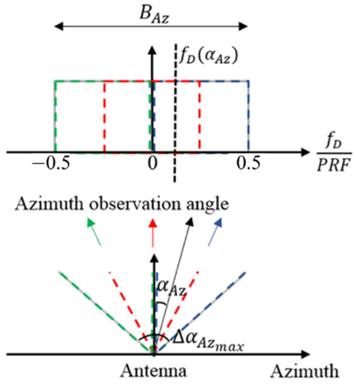
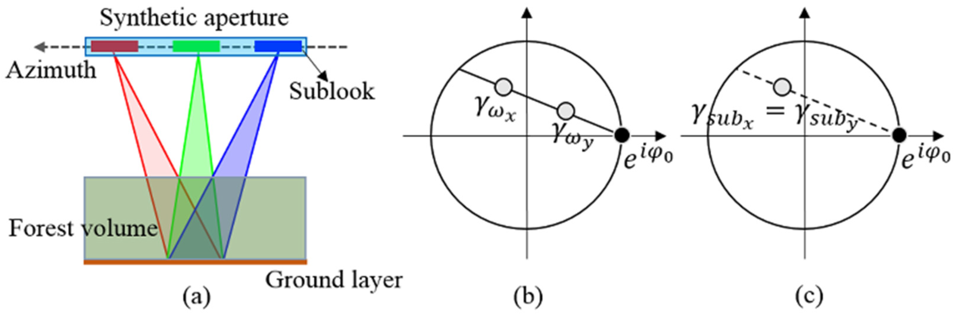
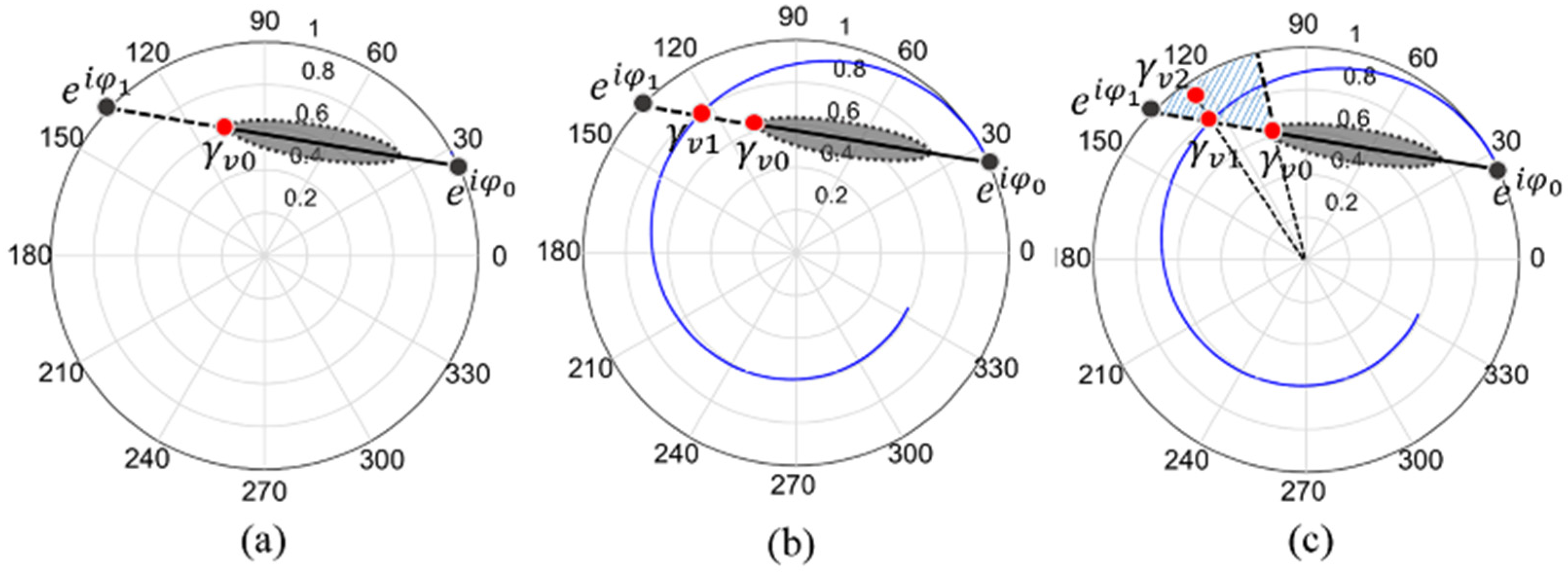
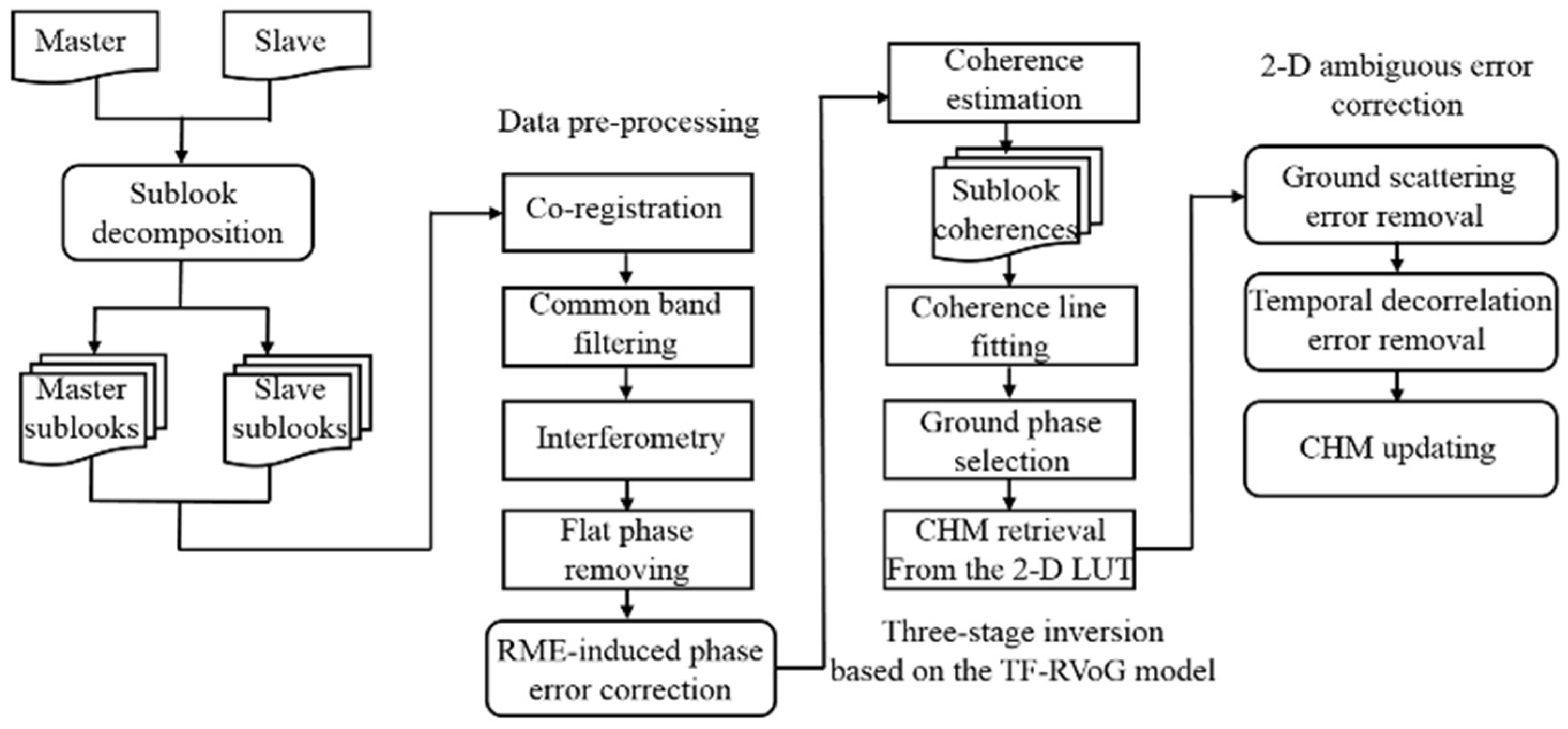
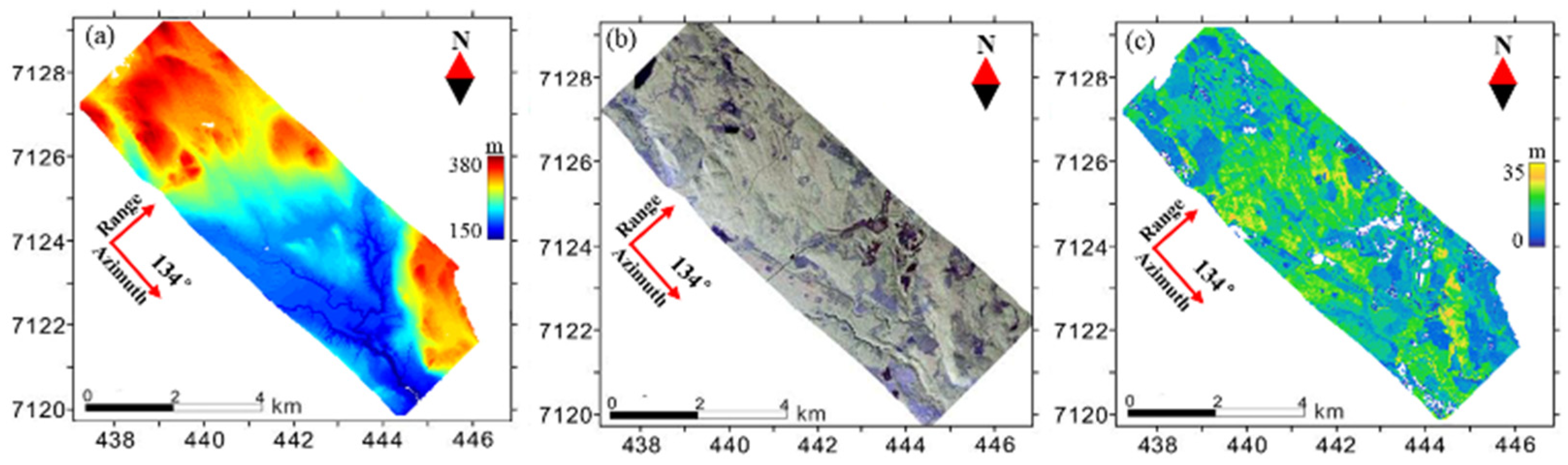
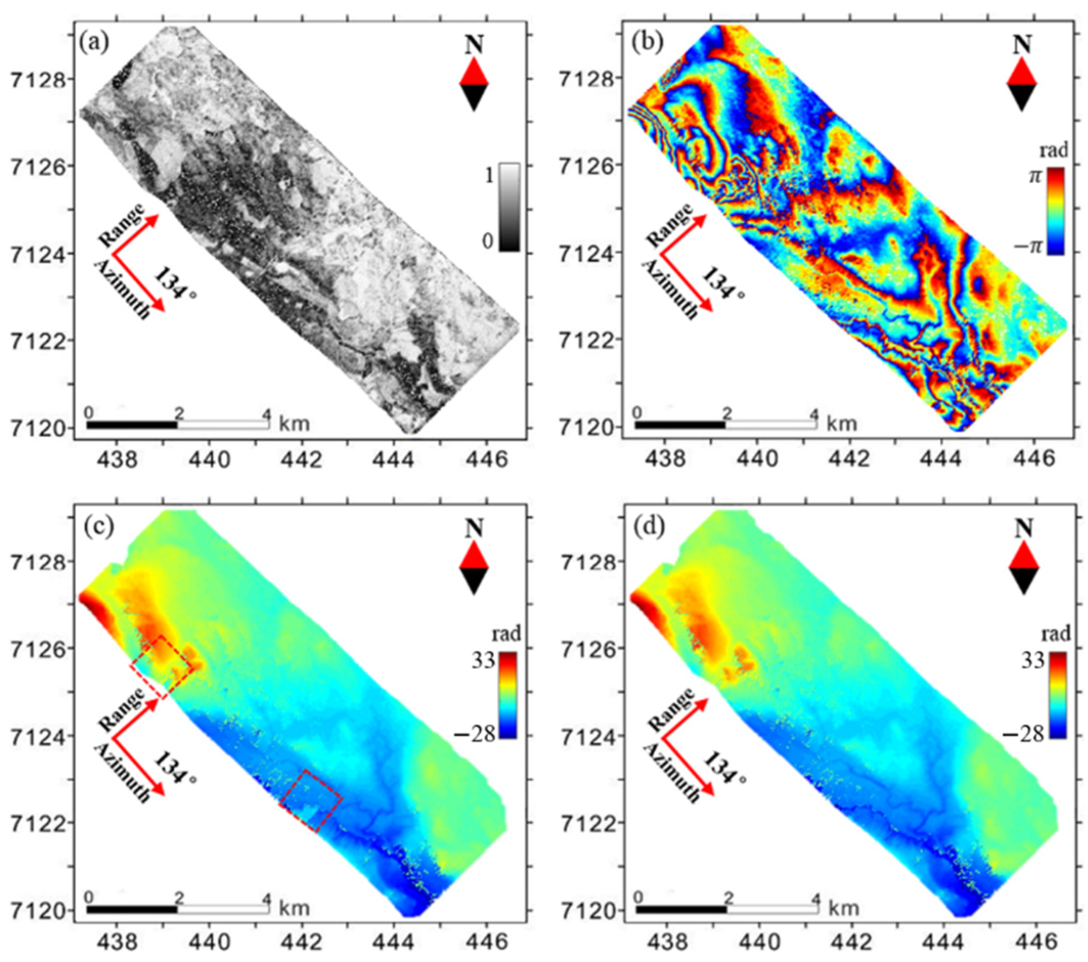
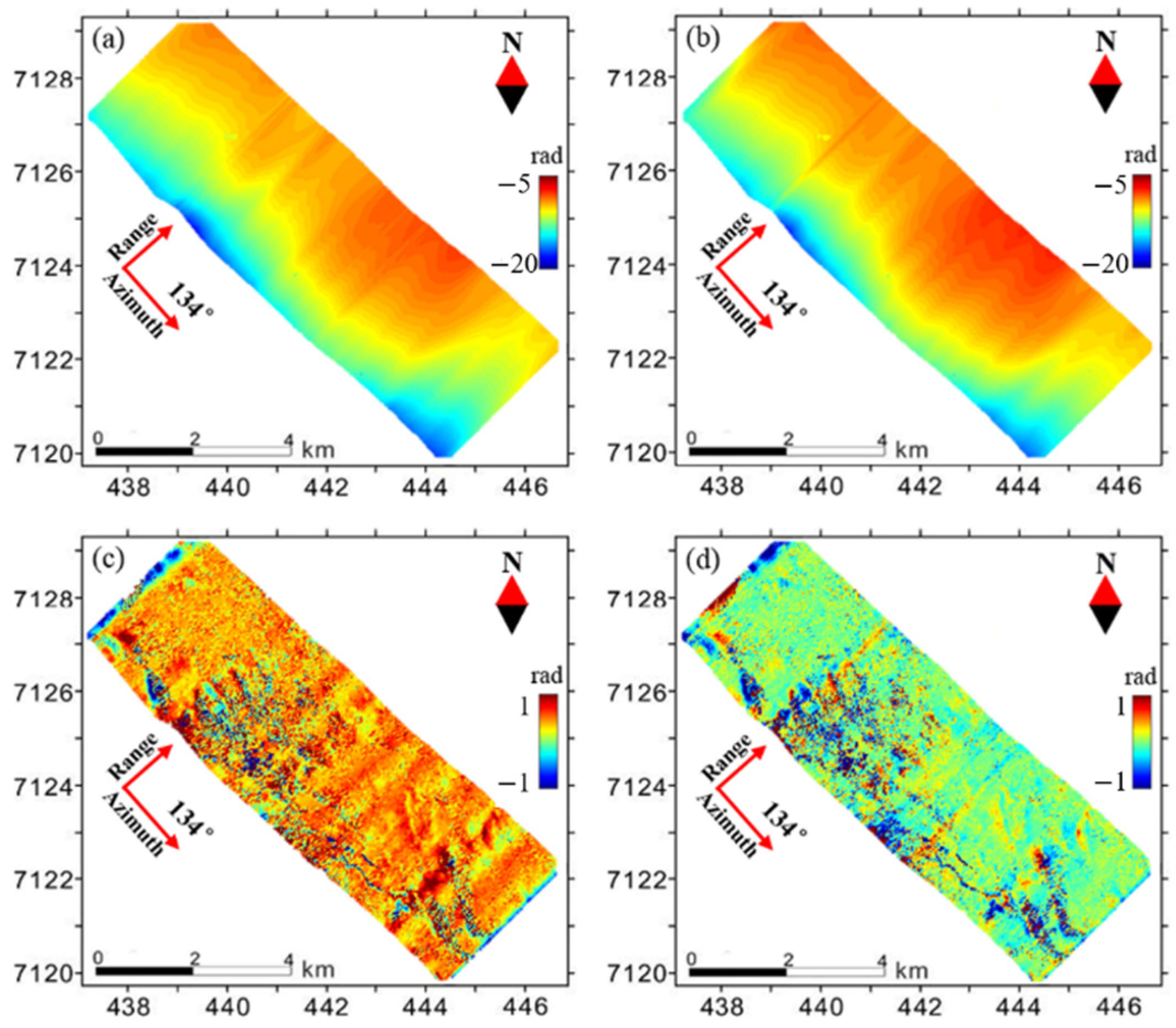
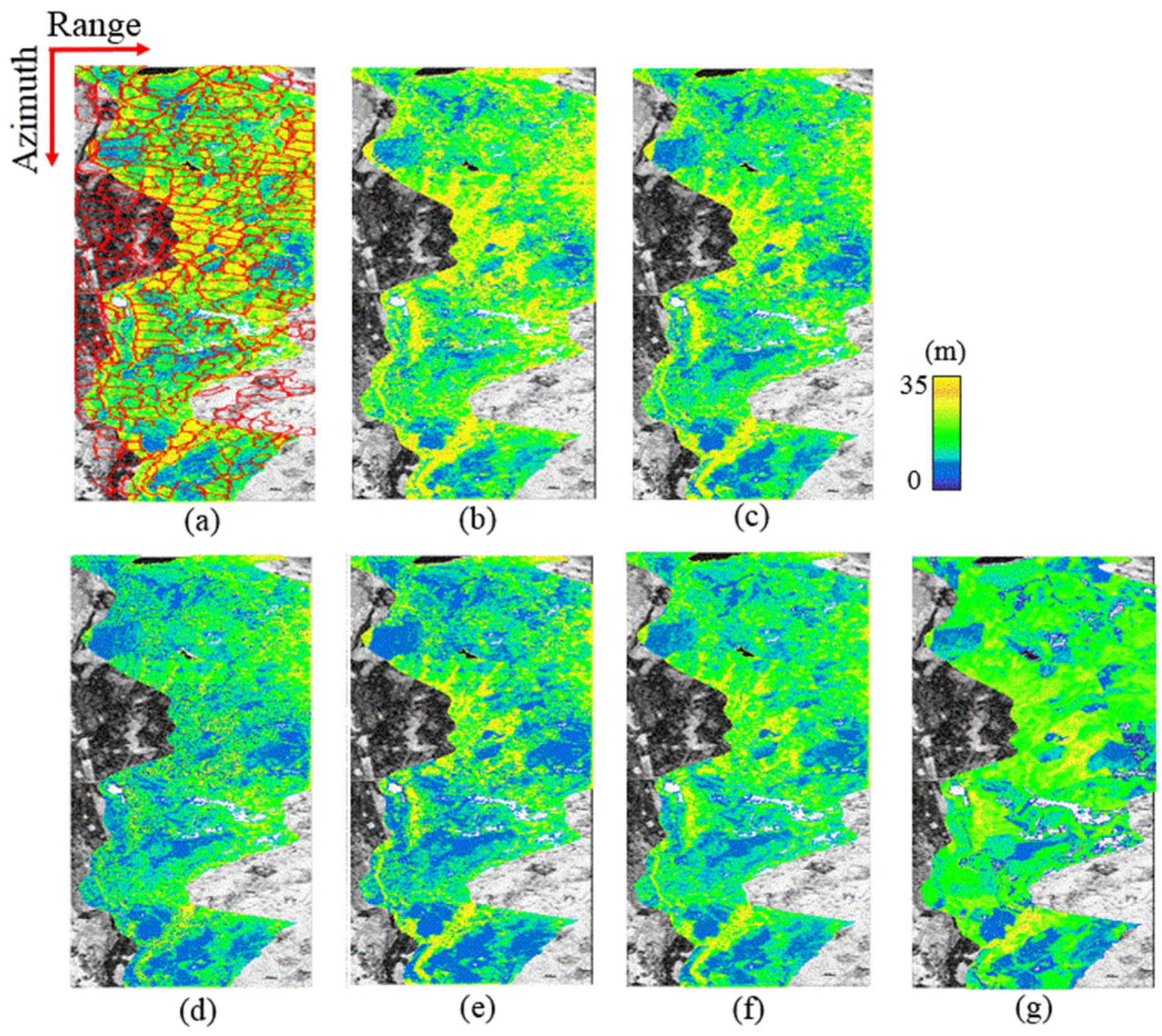
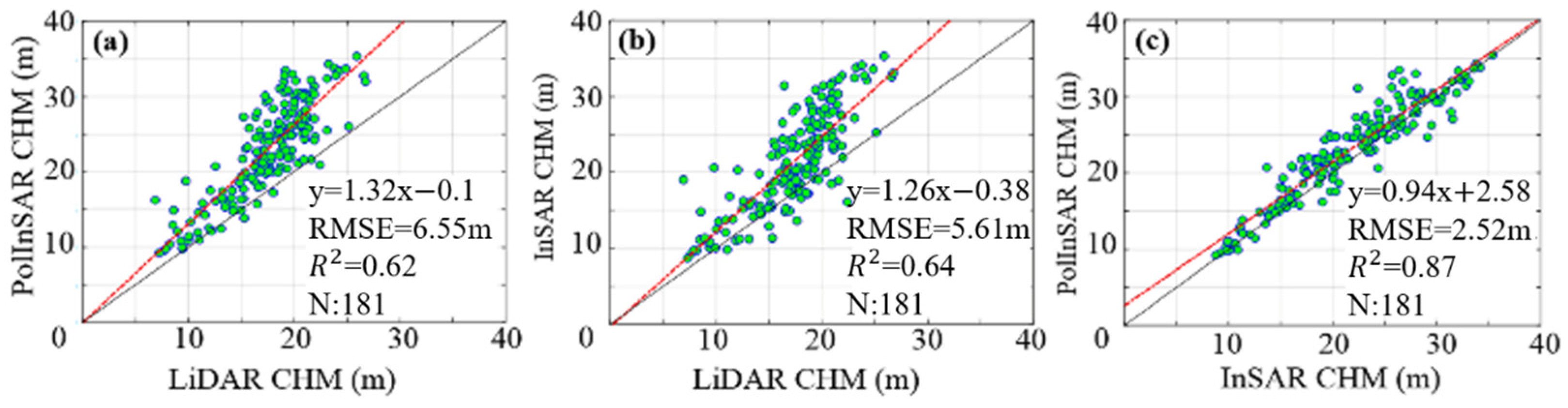
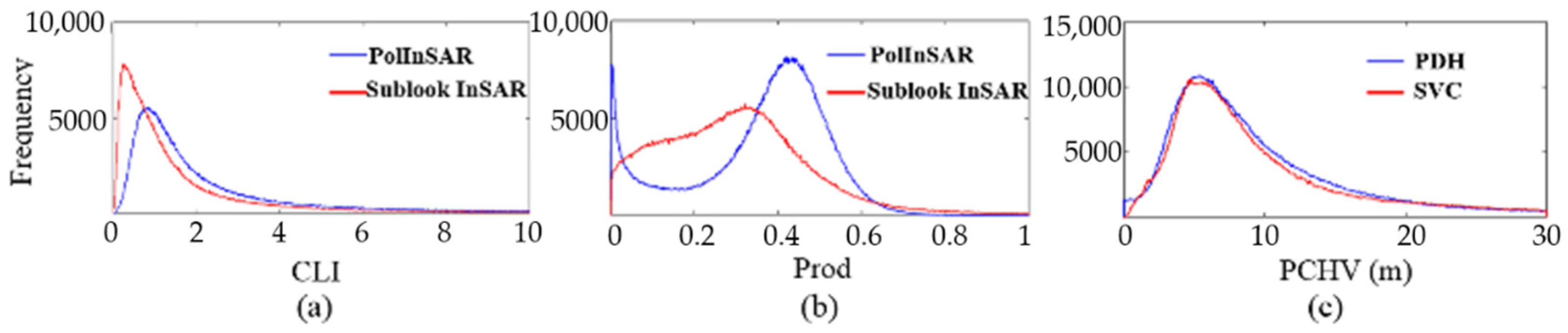
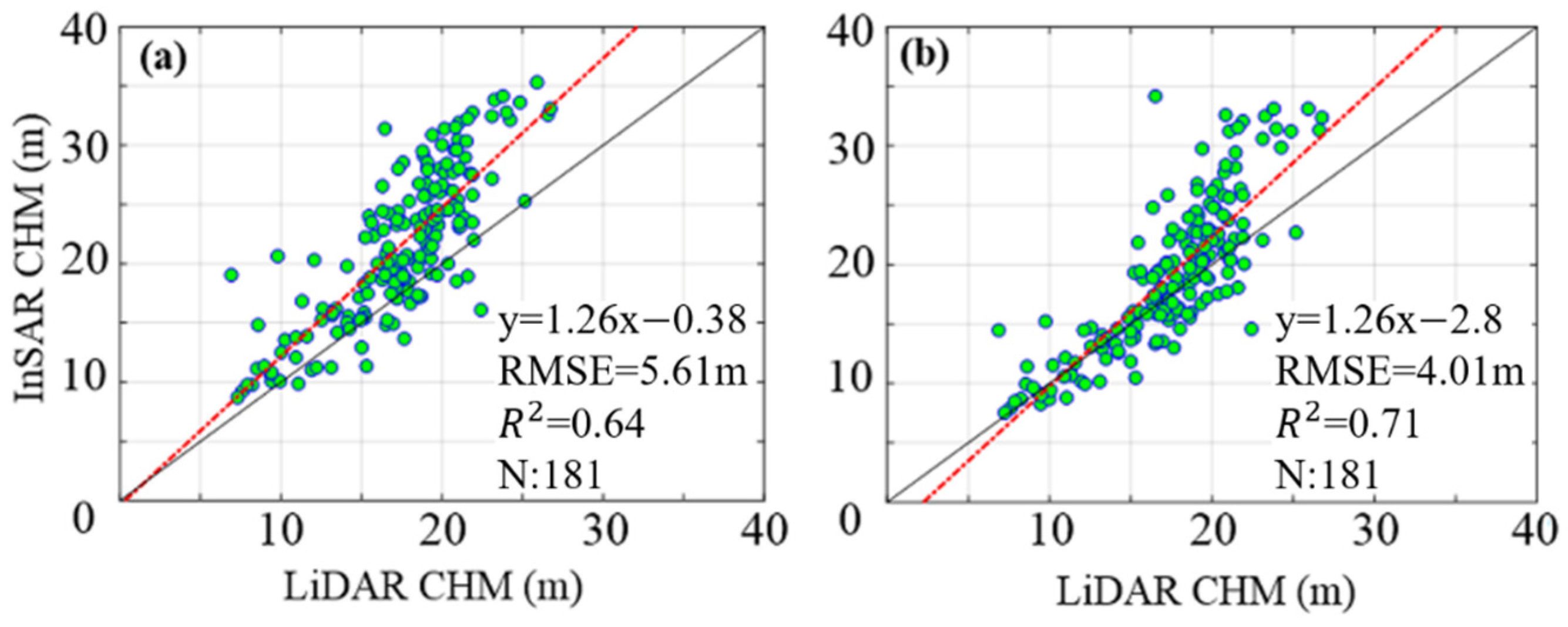
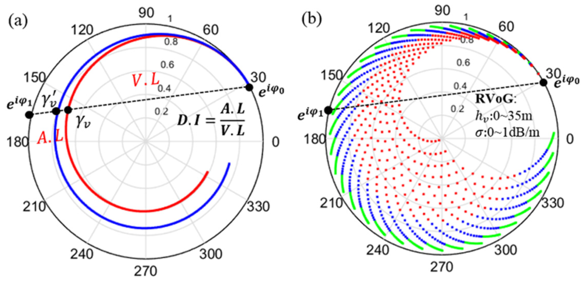
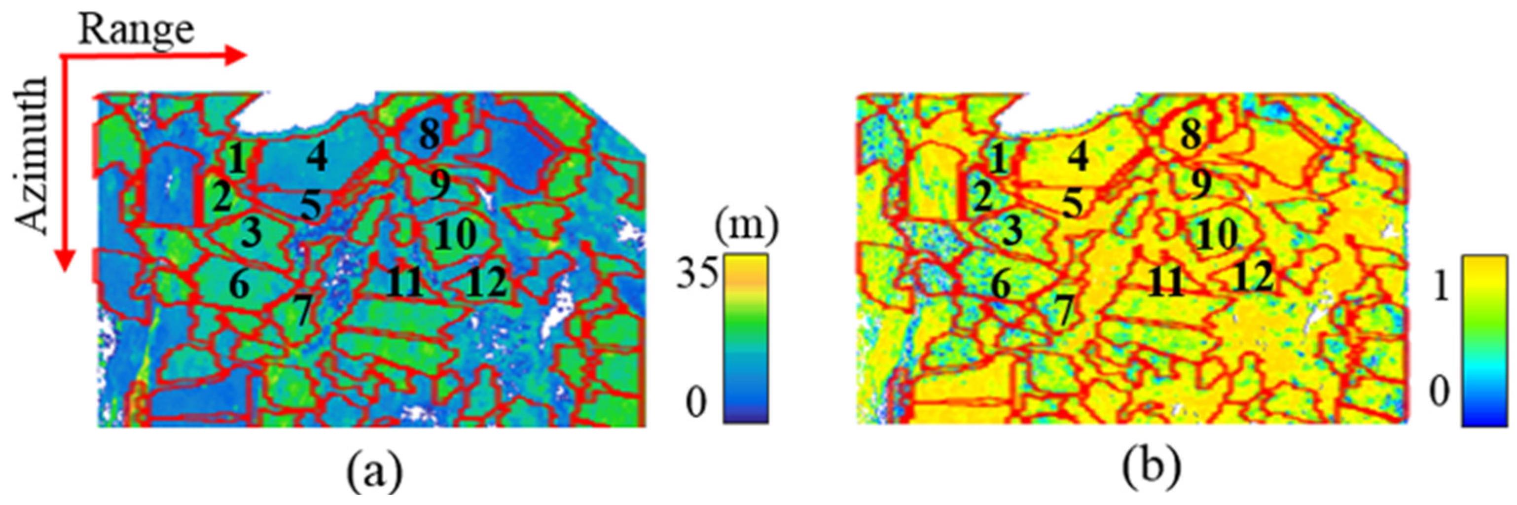
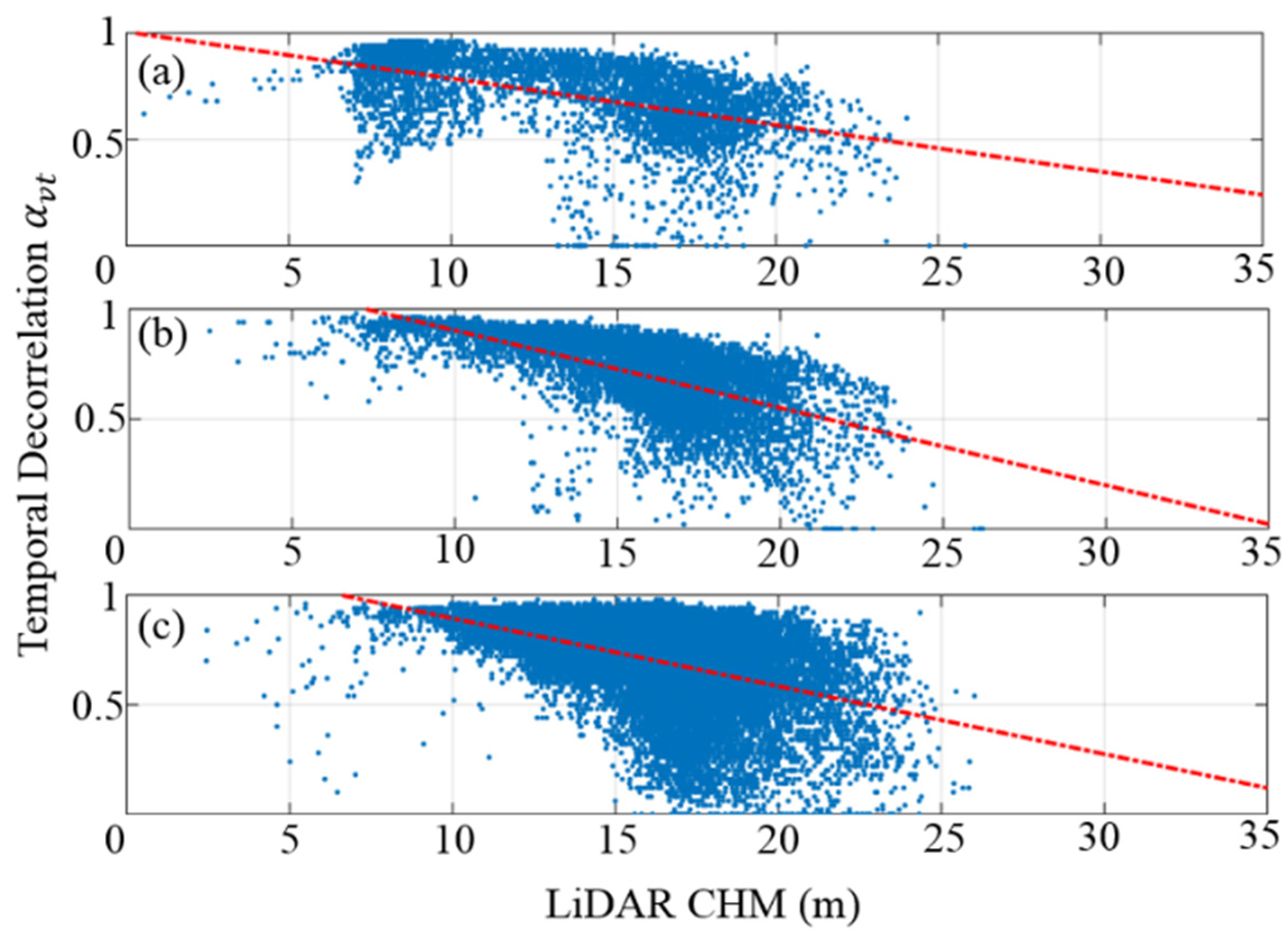
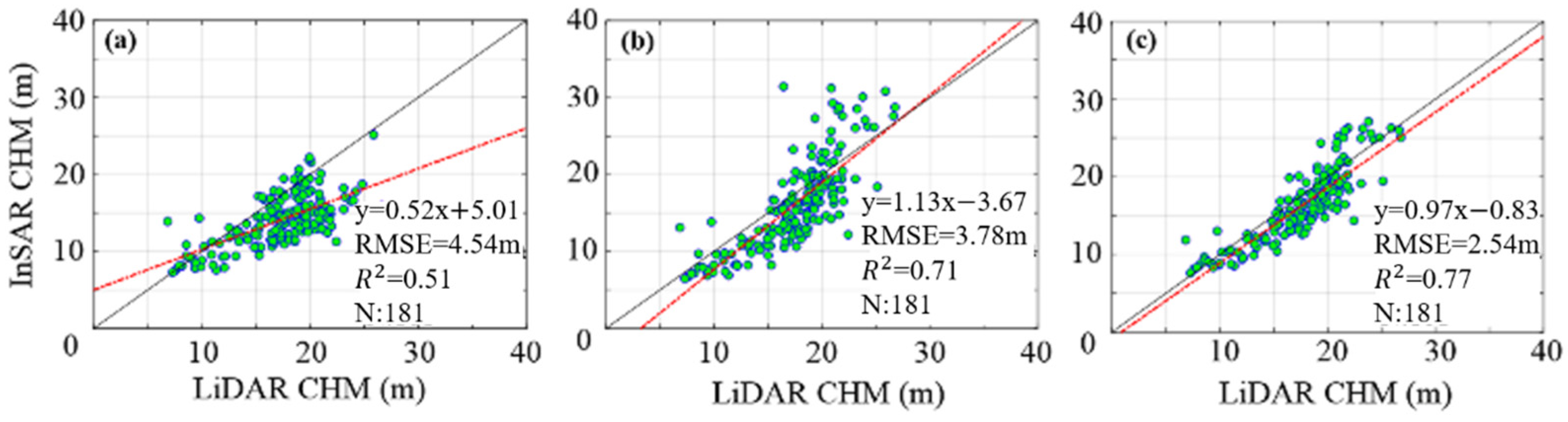
Table 1.
The Limited Extinction Coefficient BASED ON the Geometrical Index.
| Index Range | Extinction Coefficient Range (dB/m) |
|---|---|
| 0–0.4 | 0.6–1 |
| 0.4–0.65 | 0.3–0.6 |
| >0.65 | 0–0.3 |
Table 2.
Comparison of the CHMs before and after using the limited extinction coefficient.
| InSAR CHM (m) | InSAR CHM with a Limited | ||
|---|---|---|---|
| 0.4 | 14.5 | 9.5 | 0.126 |
| 0.32 | 21 | 14.5 | 0.267 |
| 0.43 | 20.5 | 14 | 0.198 |
| 0.71 | 35 | 35 | 0 |
| 0.22 | 17 | 12.5 | 0.055 |
| 0.23 | 22.5 | 15 | 0.054 |
| 2.02 | 6.5 | 6.5 | 0 |
| 0.82 | 32 | 32 | 0 |
Disclaimer/Publisher’s Note: The statements, opinions and data contained in all publications are solely those of the individual author(s) and contributor(s) and not of MDPI and/or the editor(s). MDPI and/or the editor(s) disclaim responsibility for any injury to people or property resulting from any ideas, methods, instructions or products referred to in the content. |
© 2022 by the authors. Licensee MDPI, Basel, Switzerland. This article is an open access article distributed under the terms and conditions of the Creative Commons Attribution (CC BY) license (https://creativecommons.org/licenses/by/4.0/).
Share and Cite
MDPI and ACS Style
Wang, L.; Zhou, Y.; Shen, G.; Xiong, J.; Shi, H. Forest Height Inversion Based on Time–Frequency RVoG Model Using Single-Baseline L-Band Sublook-InSAR Data. Remote Sens. 2023, 15, 166. https://0-doi-org.brum.beds.ac.uk/10.3390/rs15010166
AMA Style
Wang L, Zhou Y, Shen G, Xiong J, Shi H. Forest Height Inversion Based on Time–Frequency RVoG Model Using Single-Baseline L-Band Sublook-InSAR Data. Remote Sensing. 2023; 15(1):166. https://0-doi-org.brum.beds.ac.uk/10.3390/rs15010166
Chicago/Turabian StyleWang, Lei, Yushan Zhou, Gaoyun Shen, Junnan Xiong, and Hongtao Shi. 2023. "Forest Height Inversion Based on Time–Frequency RVoG Model Using Single-Baseline L-Band Sublook-InSAR Data" Remote Sensing 15, no. 1: 166. https://0-doi-org.brum.beds.ac.uk/10.3390/rs15010166
Note that from the first issue of 2016, this journal uses article numbers instead of page numbers. See further details here.