Article

First Demonstration of Space-Borne Polarization Coherence Tomography for Characterizing Hyrcanian Forest Structural Diversity

1
Department of Electronics and Nanoengineering, Aalto University, 02150 Espoo, Finland
2
Department of Forestry, Gorgan University of Agricultural Sciences and Natural Resources, Gorgan 49189-43464, Iran
3
Department of Earth Observation Science, University of Twente, 7514AE Enschede, The Netherlands
4
Department of Forest Sciences, University of Helsinki, 00014 Helsinki, Finland
*
Author to whom correspondence should be addressed.
Submission received: 7 December 2022 / Revised: 9 January 2023 / Accepted: 11 January 2023 / Published: 17 January 2023
(This article belongs to the Special Issue SAR for Forest Mapping II)

Abstract

:
Structural diversity is recognized as a complementary aspect of biological diversity and plays a fundamental role in forest management, conservation, and restoration. Hence, the assessment of structural diversity has become a major effort in the primary international processes, dealing with biodiversity and sustainable forest management. Because of prohibitive costs associated with the ground measurements of forest structure, despite their high accuracy, space-borne polarization coherence tomography (PCT) can introduce an alternative approach given its ability to provide a vertical reflectivity profile and spatiotemporal resolutions related to detecting forest structural changes. In this study, for the first time ever, the potential of space-borne PCT was evaluated in a broad-leaved Hyrcanian forest of Iran over 308 circular sample plots with an area of 0.1 ha. Two aspects of horizontal structure diversity, including standard deviation of diameter at breast height ( σ d b h ) and the number of trees ( N ), were predicted as important characteristics in wood production and biomass estimation. In addition, the performance of prediction algorithms, including multiple linear regression (MLR), k-nearest neighbors (k-NN), random forest (RF), and support vector regression (SVR) were compared. We addressed the issue of temporal decorrelation in space-borne PCT utilizing the single-pass TanDEM-X interferometer. The data were acquired in standard DEM mode with single polarization of HH. Consequently, airborne laser scanning (ALS) was used to estimate initial values of height h v and ground phase φ 0 . The Fourier–Legendre series was used to approximate the relative reflectivity profile of each pixel. To link the relative reflectivity profile averaged within each plot with corresponding ground measurements of σ d b h and N , thirteen geometrical and physical parameters were defined ( P 1 P 13 ). Leave-one-out cross validation (LOOCV) showed a better performance of k-NN than the other algorithms in predicting σ d b h and N . It resulted in a relative root mean square error (rRMSE) of 32.80%, mean absolute error (MAE) of 4.69 cm, and R2* of 0.25 for σ d b h , whereas only 22% of the variation in N was explained using the PCT algorithm with an rRMSE of 41.56%. This study revealed promising results utilizing TanDEM-X data even though the accuracy is still limited. Hence, an entire assessment of the used framework in characterizing the reflectivity profile and the possible effect of the scale is necessary for future studies.

Graphical Abstract

1. Introduction

Forest structure is an indicator of forest succession, development, and sustainability, which could be described by indices-based approaches [1,2]. Different aspects of stand density, species composition, horizontal and vertical tree distribution patterns, tree size distribution, and age composition characterize forest structure [2]. Thus, forest structure is an important parameter in assessing forest productivity, biomass, and especially biodiversity [3,4]. Structurally diverse forest stands with multiple canopy stories and high variation in diameter at breast height (dbh) provide potential habitats for forest-dependent species [5]. Therefore, the evaluating, retrieving, and preserving of forest structural diversity have been the main attempts to prevent biodiversity loss [6,7]. From a management point of view, the spatially explicit structural diversity maps are reasonably assumed to assist in planning conservation strategies [8]. A variety of structural diversity indices have been introduced to evaluate habitat functions and forest management planning [9,10]. However, the most common ones are structural diversity indices in horizontal and vertical dimensions based on the dbh and height [5,8,11,12,13]. They are in line with the findings of Working Group 3 of Action E43 of the European program Cooperation in Science and Technology (COST), i.e., Harmonization of National Forest Inventories (NFIs) in Europe: Techniques for Common Reporting. Hence, NFIs that have traditionally been designed for forest coverage and productivity assessment can represent a main component of the global biodiversity monitoring network by introducing easy-to-measure structural diversity indices [6].
A wide range of applications needs structural diversity information. Each of them has specific spatio-temporal requirements that cannot be satisfied by ground measurements. In addition to the costs associated with ground measurements, they are labor intensive and only cover local areas. In contrast, remote sensing technologies, especially the rapid development in synthetic aperture radar (SAR) technology, can overcome some of these limitations by measuring forests in a cost-effective and reliable manner at a large scale [14]. Many studies have been conducted based on SAR backscattering coefficients [15,16,17,18,19]. Nevertheless, SAR systems provide 2D images that only represent a projection of 3D scene scattering properties along the elevation direction that contradicts the 3D reality of forest structure [20]. One of the most recent innovations in SAR processing is the extending of imaging process from 2D into 3D using multi-baseline datasets [21]. SAR Tomography (TomoSAR) is an advanced interferometric SAR (InSAR) technique based on multi-baseline observations. It can separate scattering contributions at different heights within the same slant range azimuth resolution cell and has emerged for the investigation of the forested area as a main approach [22,23]. However, TomoSAR application using repeat-pass space-borne acquisitions is often hindered by temporal decorrelation. Additionally, atmospheric propagation delay is a dominant phase noise in space-borne SAR data [24]. For these reasons, tomography studies have been mostly conducted on airborne datasets [25,26,27,28].
Polarization coherence tomography (PCT) is an alternative approach when a limited number of acquisitions are available. It uses a priori knowledge of height and ground phase for approximating unknown vertical reflectivity profile by the Fourier–Legendre series [29]. A few studies have conducted PCT technique for forestry applications using experimental airborne datasets in specific areas [30,31,32,33,34,35,36]. For instance, Luo et al. [37] have estimated forest aboveground biomass (AGB) using single-baseline E-SAR L-band PolInSAR data in a mountainous mixed forest of southern Germany. They defined nine parameters to characterize the mean reflectivity profile over 20 stands. The results showed higher sensitivity of tomographic parameters for forest AGB estimation than PolInSAR-derived forest height. Following the mentioned study, similar results were obtained by Li et al. [34] at the stand-level, where tomographic forest height individually, and in combination with other parameters derived from vertical reflectivity profile, resulted in higher forest AGB estimation accuracy than PolInSAR-derived forest height, 50.76, 39.98, and 71.80 Mg.ha−1, respectively. In another study, Zhang et al. [35] examined the potential of single baseline Bio-SAR P-band data for forest AGB estimation in northern Sweden. They introduced a new tomographic height based on analyzing loss backscatter power, which resulted in an improved RMSE of 18.325 Mg.ha−1 when combined with the nine parameters defined by Lu et al. [34], whereas Neuman et al. [38] reported an RMSE of 23 Mg.ha−1 using the PolInSAR technique in the same study area.
However, the large-area estimation of forest structural parameters is still challenging. By launching TerraSAR-X and TanDEM-X platforms, the first space-borne single-pass interferometer has formed [39]. They provide high-resolution polarimetric acquisitions with a temporal baseline of zero (bistatic mode) and near-zero (pursuit monostatic) that could be a compensation for the key issues of space-borne PCT (see [40]). Although X-band is a rather suboptimal frequency in forest studies because of the lower penetration depth into the canopy, the sensitivity of InSAR measurements at the X-band to forest vertical structure has been shown for cases of both single-baseline [41,42,43] and multi-baseline [39,44,45]. Such results stimulate more attempts to investigate X-band potentials in a wide range of forest sites. Praks et al. [30] demonstrated the sensitivity of PCT accuracy to the initial values of height and especially the ground phase. Their results showed initial values derived from airborne laser scanning data (ALS) have improved the performance of fully polarimetric repeat pass L-band PCT than when they are derived from the random volume over ground (RVoG) model [46]. On the other hand, the standard DEM mode of the TanDEM-X interferometer is single-pol operated in HH (or VV) polarization. Consequently, additional research would also be necessary for parametrizing complex coherence [30,43]. In this study, for the first time ever, single-pol (HH) TanDEM-X interferometer was used for approximating the vertical reflectivity profile of the Hyrcanian forest using the PCT technique. In addition, multiple prediction techniques, each based on different underlying assumptions and complexity, have been used to predict forest structural parameters [47,48,49,50]. Regression models are among them with demonstrated capability in predicting structural attributes while the results may be poor in the cases of weak regression relationship and/or insufficient ground sample sizes. Non-parametric algorithms, some of which use machine learning, have been shown to be an alternative approach. Therefore, the main research question is how accurately the variation in forest reflectivity profile can describe the horizontal structural diversity of the Hyrcanian forest, including the standard deviation of dbh ( σ d b h ) and the number of trees ( N ). Moreover, we compare prediction algorithms of multiple linear regression (MLR), k-nearest neighbors (k-NN), random forest (RF), and support vector regression (SVR) in their performances. Our study provides insight into the feasibility of TanDEM-X interferometer in studying forest structure diversity by approximating the vertical reflectivity profile.

2. Materials and Methods

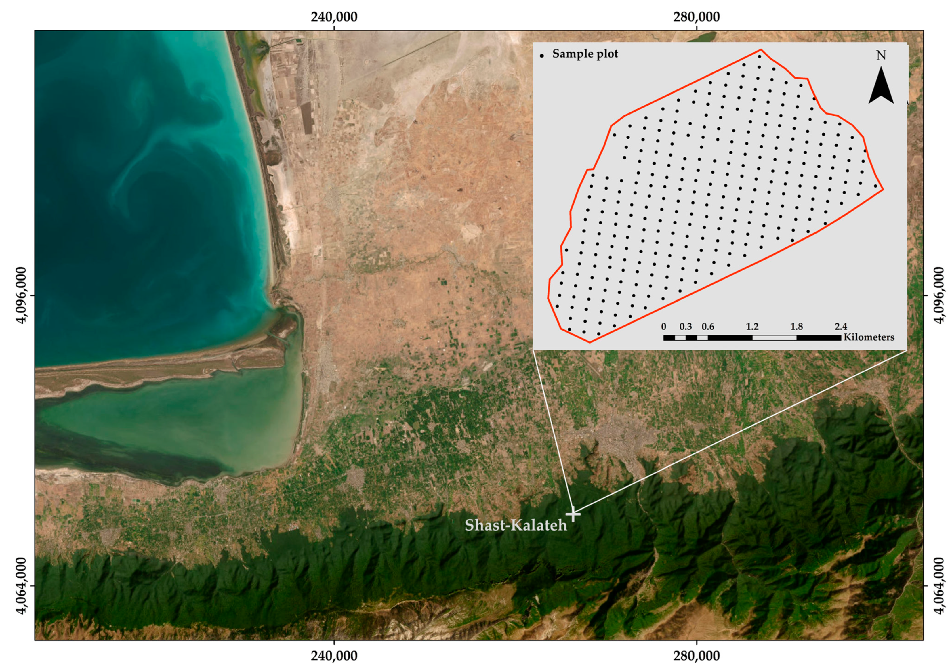
2.1. Site Description

The study area is located in the Shast-Kalateh forest, which is a part of the temperate deciduous Hyrcanian forests of Iran on the shores of the Caspian Sea (Figure 1). It includes logged managed and unmanaged forests dominated by Parotia persica, Carpinus betulus, Fagus orientalis, and Diospyrus lotus. The area spreads over 1100 ha and is bounded by 54°31′–54°42′ E and 36°73′–36°78′ N. The elevation ranges from 270 to 740 m above sea level and is characterized as a middle humid climate with mean annual precipitation of 649 mm and a mean annual temperature of 15.4 °C.

2.2. Field Data and Structural Diversity Indices

The field survey was conducted across 308 circular sample plots with a size of 0.1 ha (radius = 17.84 m) in 2011 [51]. A systematic sampling design on the grid size of 150 × 200 m with a random starting point was used to locate sample plots (Figure 1). The plot center coordinates were also estimated by the differential global positioning system (DGPS). All the trees with a diameter at breast height (dbh) of at least 12.5 cm were measured for the dbh with a caliper, height with a Vertex (VL 402), and tree species. Accordingly, the basal area, as a cross-sectional area of a tree that is assumed to be circular, and volume based on species-specific local volume tables with dbh and height as predictor variables were calculated. Table 1 shows the summary of plot-level field data, including basal-area-weighted mean dbh and height, mean volume, the standard deviation of dbh, and the number of trees.
A variety of structural indices have been developed to measure the diversity of forest stands in the literature [9,10,52,53]. In this study, two commonly used structural diversity indices of standard deviation of dbh ( σ d b h , Equation (1)) and the number of trees ( N ) were used (Table 1).
  σ d b h = n = 1 N ( d b h n d b h ¯ ) 2 N 1
where n denotes the trees and N is the number of trees in sample plot. The following criteria were met in the selection of indices. First, they are easy to measure, reliable, and relevant to biodiversity [9,53,54,55,56]. The stands with high variation in size and number of stems are prone to having large distributions of forest-dependent species. Second, both the indices can be estimated from the national forest inventory (NFI) dataset, which can be an advantage for future global biodiversity monitoring networks [57,58]. Third, these are indicators introduced in the primary international processes dealing with biodiversity and sustainable forest management (e.g., Convention on Biological Diversity (CBD), Forest Europe, Streamlining European Biodiversity Indicators 2010 of the European Environmental Agency, and the Montréal Process).

2.3. TanDEM-X Data

Bistatic single polarized (HH) TanDEM-X data was acquired on February 2011 in strip map mode. It was collected at ascending pass with look angles of 46.22° m and height of ambiguity (HOA) of 40.39 m. The delivered product was in a co-registered single-look slant range complex (CoSSCs) format with range and azimuth spacing of 1.36 and 2.16 m. By calculating the normalized complex interferometric coherence of s 1 and s 2 signals received at either end of the baseline ( γ ˜ , Equation (2)), the interferogram was generated and filtered to reduce speckle noises.
γ ˜ = E { s 1 . s 2 * } E { | s 1 | 2 } .   E { | s 2 | 2 }
where * represents the complex conjugate, E is the expectation, and 0 < | γ ˜ | < 1 [46]. Furthermore, the flat earth effect was subtracted from the phase image to obtain valid height information.

2.4. Airborne Laser Scanning Data

ALS data were collected in 2011 across the study area. Riegl LMS Q560 were used to collect row data at a mean flying altitude of 1000 m above sea level under leaf-on condition. The pulse repetition frequency of 240 kHz and a scan angle of 22.5°–30° resulted in an average density of 4 pulses m2. The digital terrain model (DTM) was generated using the Kraus and Pfeifer [59] algorithm with the triangulated irregular network (TIN) interpolation. Its accuracy was investigated based on 90 ground control points and a 40 cm accuracy was achieved. TIN interpolation was also used to obtain DSM from the highest point within 1 m grid, and, simply by subtracting DTM from DSM a canopy height model was generated.

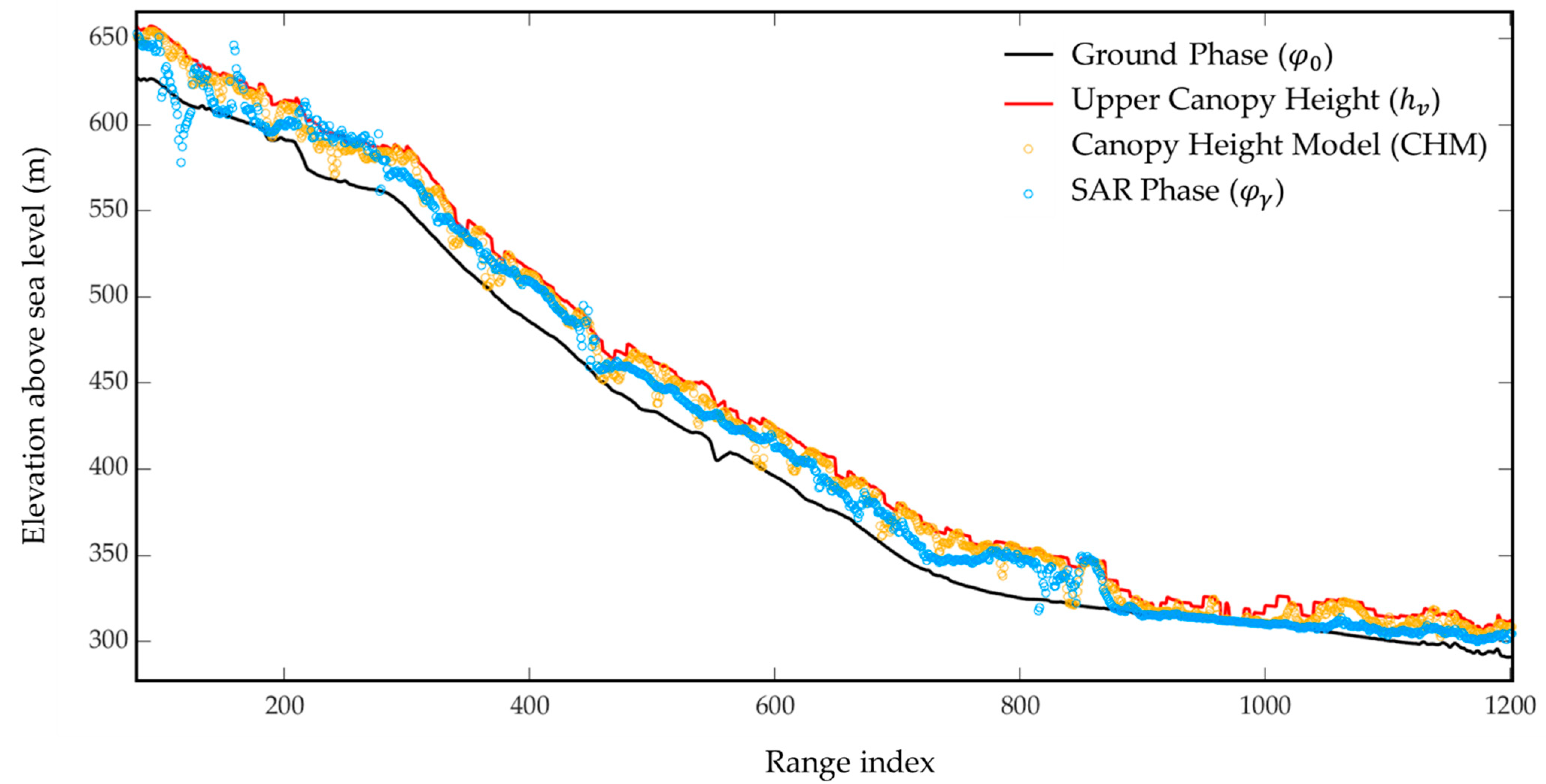
2.4.1. Forest Height and Ground Phase Estimation

Upper canopy height is a standard forestry parameter, defining the basal area-weighted height average of the 100 highest trees per hectare. Many studies showed its relevance to volume height measured by SAR data [30,43,60]. Considering the laser penetration into the forest, an estimate of upper canopy height was achieved by filtering CHM to the highest point in a 10 × 10 m window, called h v . This allows compensation for underestimated lidar forest height estimation [60,61]. Finally, DTM and H100 were converted to slant range TanDEM-X coordinate to use as initial values of the PCT algorithm (Section 2.5).
Moreover, unfiltered DTM was wrapped into the ground phase φ 0 using SAR vertical wavenumber k z and the train elevation h D T M (Equation (3)) [30,43].
φ 0 = k z ( h D T M + h f ) + f
where h f and f are unknown parameters. They were computed by fitting obtained φ 0 and SAR phase φ γ ˜ on open areas with sufficient high coherence, i.e., | γ ˜ | > 0.90 by minimizing the cost distance function E using the Nelder–Mead simplex method (Equation (4)). Figure 2 shows a view of φ 0 , φ γ ˜ , and h v along a transect in slant range coordinates. As you can see, the ground phase has good accordance with the dataset, especially in the open areas.
E = | e i φ D T M e i φ γ ˜ | 2

2.5. Polarization Coherence Tomography (PCT)

PCT employs the variation of the complex interferometric coherence γ ˜ to reconstruct forest vertical structure function in the penetrable depth of volume scattering (Section 2.3). Moreover, the initial values of h v and φ 0 , estimated in Section 2.4.1, are used in the reconstruction. According to the RVoG scattering model, in forested areas with the randomly vertical distribution of scatterers, γ ˜ is formulated in Equation (5) [62].
γ ˜ ( w ) = e i φ 0 0 h v F ( z ) e i k z z d z 0 h v F ( z ) d z       0 | γ ˜ | 1
where w is the polarization unitary vector, φ 0 is the ground topographic phase, h v is the vegetation height, k z is the vertical wavenumber, and F ( z ) is the vertical structure function. F ( z ) is defined as the vertical variation in microwave reflectivity at a point in 2D radar image. We reconstructed a new structure function, called F ( z ´ ) , based on the dependency between γ ˜ ( w ) and F ( z ) in the absence of temporal decorrelation, as shown in Equation (5) [63]. For this purpose, φ 0 was removed and the integral range normalized to derive Equation (6). Therefore, F ( z ´ ) can be expanded as simpler functions of the Fourier–Legendre series. (Equation (7)) [29].
γ ˜ ( w ) = h v 2 e i k z h v 2 1 1 ( 1 + F ( z ´ ) ) e i k z h v 2 z ´ d z ´ h v 2 1 1 ( 1 + F ( z ´ ) )   d z ´ ,   z ´ = 2 z h v 1
F ( z ´ ) = n a n p n ( z ´ ) ,   a n = 2 n + 1 2 1 1 F ( z ) ´ p n ( z ) ´ d z ´
where p n ( z ´ ) denotes Legendre polynomials with the vertical variable of z ´ , and a n denotes unknown Legendre coefficients. Then, γ ˜ ( w ) can be directly related to the unknown coefficients of Legendre by Equation (8) [63]:
γ ˜ ( w ) e i k v = γ ˜ k = f 0 + a 10 f 1 + a 20 f 2 + a n 0 f n
where f ( n ) are weighted integrals over the Legendre polynomials, which are a function of a single parameter k v = k z h v 2 . As it can be seen, γ ˜ ( w ) is the algebraic sum of series structure functions. In our single baseline case, the series was truncated for the second order, i.e., only f 0 , f 1 , and f 2 were computed (Equation (9)).
f 0 = s i n k v k v
f 1 = i ( s i n k v k v 2 c o s k v k v )
f 2 = 3 c o s k v k v 2 ( 6 3 k v 2 2 k v 3 + 1 2 k v ) s i n k v
Although improved tomographic resolution can be achieved by multi-baselines, it increases the number of unknown parameters and computational complexity [35]. Hence, single baseline PCT is the simplest way of forest vertical structure approximation, which only requires a 10 and a 20 . They were estimated through matrix inversion, as shown in Equation (10). Finally, the normalized structure function for each pixel at a known layer depth of h v was obtained using estimated Legendre coefficients (Equation (11)) [40]. We approximated the relative tomographic profiles with 0.2 m intervals in vegetation height [34,35,64,65].
[ 1 0 0 0 f 1 0 0 0 f 2 ] [ a 00 a 10 a 20 ] = [ 1 I m ( γ ˜ k ) R e ( γ ˜ k ) f 0 ]
[ f ] a _ = g _ a ^ _ = [ f ] 1 g _
F ^ ( z ´ ) = 1 h v { 1 a ^ 10 + a ^ 20 + 2 z ´ h v ( a ^ 10 3 a ^ 20 ) + a ^ 20 6 z ´ 2 h v 2 }               0 z ´ h v  

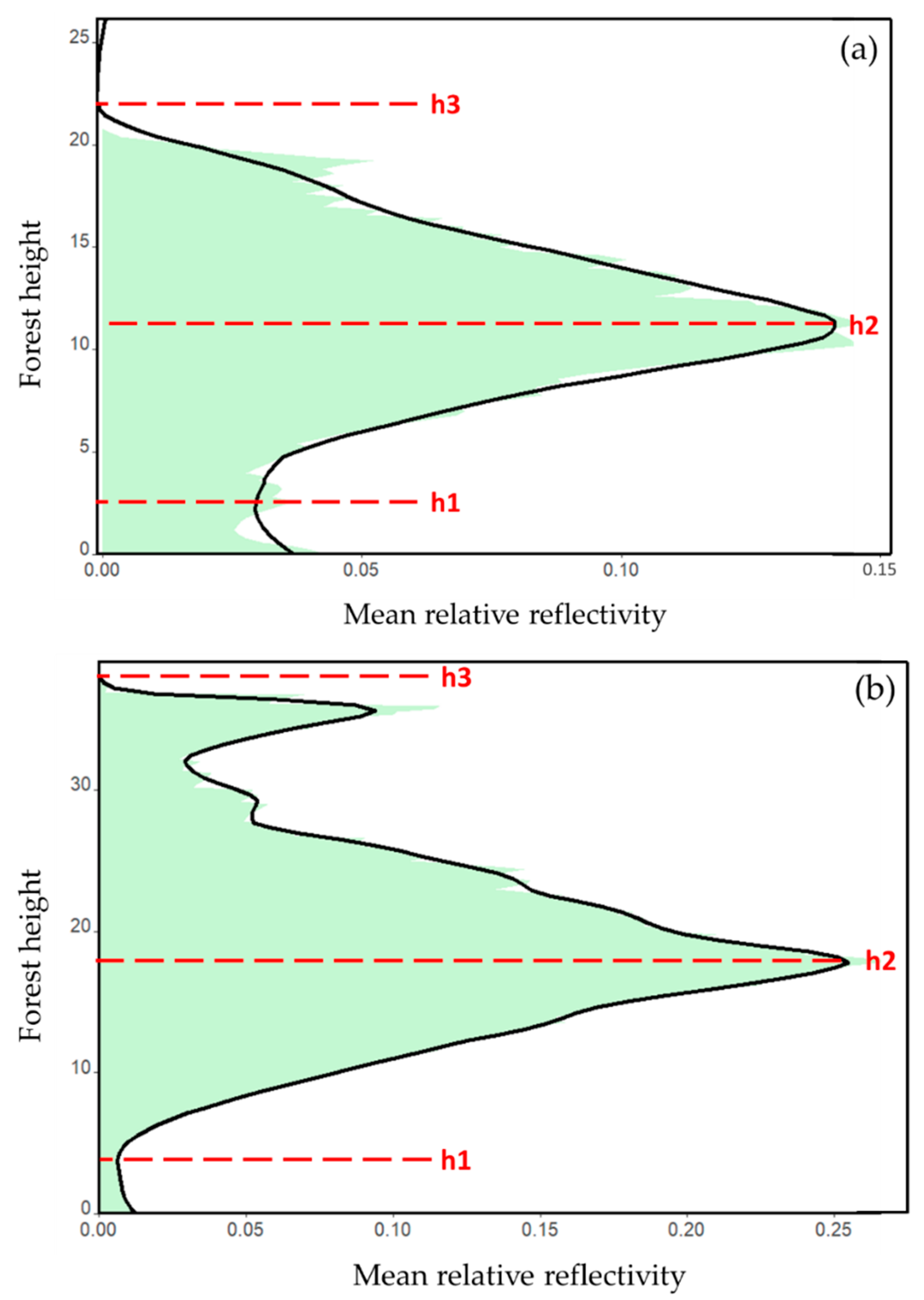
Characterizing Tomographic Profiles

The objective of this section was to define a framework to link tomographic profiles with forest structural diversity. A direct transformation of ecology and forestry metric into PCT profile is a difficult challenge as individual tree measures are usually impossible to retrieve from tomographic profiles [66]. In this study, we mainly extracted geometric descriptors of the tomographic profile based on the method originally described by Lue et al. [37]. The arithmetic average of tomographic profiles was computed for the pixels inside each plot to further plot-level analysis [34,35,37]. Because of irregularly obtained mean profiles, i.e., the highly varied vertical reflectivity between adjacent pixels, we fitted the gaussian model for further use. Two plot-level mean relative reflectivity profiles are shown in Figure 3a, and b as examples corresponding to low ( σ d b h = 9.38 cm) and high ( σ d b h = 39.65 cm) structural diversity, respectively. By dividing the curve into two envelopes and defining h1, h2, and h3, ten geometrical parameters were defined ( P 1 P 10 , Table 2).
The first envelope comprised the reflectivity values between h1 and h3 corresponded to the canopy phase zone, where h1 is the inflection point between the lower and upper parts of the mean relative reflectivity curve and h3 is considered as a height with mean relative reflectivity closest to 0.001. The h2 corresponds to the height position where the mean relative reflectivity is maximum. Notably, the data between 0 and h2 constitutes the second envelope. Moreover, the mean relative reflectivity profiles were also characterized as reflectivity power distribution, according to Zhang et al. [35], and P 11 was computed. It is a physical scattering attenuation parameter obtained by introducing the area between h2 and h3 as a reflectivity power loose zone and above h3 that is mostly contributed by the noise (Table 2). In addition, the location of 3D reflectivity peaks appears significantly more robust to reflectivity variation induced by system features and environmental conditions [66]. Hence, we used the number and 3D distribution of reflectivity peaks for structure diversity estimation that were estimated by package splus2R of R ( P 12 P 13 , Table 2) [67].

2.6. Prediction Algorithms

Multiple linear regression (MLR) and three non-parametric algorithms, k-nearest neighbors (k-NN), random forest (RF), and support vector regression (SVR), were employed to estimate plot-level forest structural diversity of σ d b h and N using P 1 P 13 . These algorithms and tuning parameters are described briefly below.
MLR algorithm was conducted with the stepwise AIC (Akaike information criterion) method to obtain the best combination of predictors to estimate forest structural diversity. The algorithm can treat the problem of collinearity and evaluation of predictor variables using leave-k-out stepwise AIC and clustering input variables [47].
The k-NN has been found as the most popular technique in remote sensing-assisted forest attribute prediction [48,68,69]. To predict ith population unit by the k-NN algorithm, a linear combination of observation in population units in a k nearest sample units (neighbors) in the feature space is calculated [68]. In this study, the rectangular kernel (standard unweighted k-NN) with k values ranging from 1 to 20 was considered. Additionally, four different distance metrics of Euclidian, Manhattan, Chebyshev, and Euclidian squared were compared to optimize k-NN algorithm [70].
RF is a widely used prediction algorithm based on regression trees and has been shown to be useful in reducing systematic errors and overfitting [49]. In this algorithm, the regression trees continue to grow until a minimum error in the aspect of response variable is achieved. All regression trees were implemented in a range of square root of the number of predictor variables ± 2 (F).
SVR assumes a unique relationship between each set of predictor variables and response variables and that the grouping among predictor variables is sufficient in formulating prediction rules [71,72]. This task is accomplished by hyperplanes in multi-dimensional space built from axes, representing predictor variables [50]. Here, kernels of linear, polynomials of degrees 2 and 3, radial base function, and sigmoid were compared in terms of prediction accuracy. A grid search approach based on gradient descent convergence is applied for optimizing SVR parameters, including cost (C), which regularized the slack from observation-to-kernel margin [50].

2.7. Accuracy Assessment

We used leave-one-out cross validation (LOOCV) to train prediction models and validation. In this method, the number of folds is equal to the number of sample plots in dataset. So, the learning algorithm is applied to each sample once that is withheld as a validation sample, while the remaining samples are used in training the model [73,74]. Although LOOCV ignores the independence requirement for accuracy assessment, it improves the reliability of accuracy assessment by reducing the random error caused by splitting sample data into train and test subsets [75,76,77]. All model predictions were evaluated by the absolute and relative root mean square error (RMSE), mean absolute error (MAE), and pseudo-R2 (R2*) (Equations (12)–(16)).
R M S E = i n ( y ^ i y i ) 2 n
r R M S E = R M S E y ¯ × 100
M A E = i n | y ^ i y i | n
r M A E = M A E y ¯ × 100
R 2 * = i n ( y i y ¯ ) 2 i n ( y ^ i y i ) 2 i n ( y i y ¯ ) 2
where y ^ i is the predicted value, y i is the observed value, y ¯ is the mean of observed values, and n is the sample size.

3. Results

3.1. Correlation Analysis

Table 3 shows the correlations of known coherency, initial value of h v , and Legendre coefficients with σ d b h and N at sample plots. Moreover, the thirteen parameters extracted from the mean relative reflectivity profile were included in the correlation analysis (Table 3). As can be seen, some extracted parameters were meaningful when compared with a 10 and a 20 as intermediate products of PCT and coherency itself. However, upper canopy height showed the highest correlation of 0.4 with σ d b h . On the other hand, PCT parameters were more gainful to correlate with N when compared with h v . Generally, P 9 , P 10 , P 11 , P 12 , and P 13 are common PCT parameters with the highest correlation with σ d b h and N .

3.2. Model Developments for Prediction of σ d b h

Table 4 shows the results of σ d b h prediction with different algorithms of MLR, k-NN, RF, and SVR. The best MLR algorithm (AIC = 1085.23) predicted σ d b h with rRMSE = 33.09% and R2* = 0.25. Among different distance metrics of k-NN, Manhattan with optimum k = 18 had the best performance for predicting σ d b h . It resulted in an RMSE of 5.99 cm (32.80%) (Figure 4). Whereas we did not find any obvious difference in σ d b h prediction accuracies by changing the number of F predictor variables in each tree node. Although, the RF model with F = 6 had marginally better accuracy than the others with an RMSE of 5.99 cm while explaining 25% of the σ d b h variation in our study area. It is worth mentioning that P 11 , P 13 , P 9 , P 10 , and P 3 are the most important variables according to the RF algorithm. SVR with optimum RBF kernel was able to predict σ d b h with rRMSE of 33.09%, and rMAE of 25.44% that had a similar performance to what was obtained with the MLR algorithm.

3.3. Model Developments for Prediction of N

The performance of MLR and non-parametric algorithms of k-NN, RF, and SVR in predicting N are shown in Table 5. The best model of MLR with AIC of 1344.05 was able to predict N with an MAE of 69.19 n ha−1 and R2* of 0.16. Manhattan with an optimum number of k = 18 led to better results when compared to the other distance metrics of Euclidian, Euclidian squared, and Chebyshev (rRMSE = 41.56%, R2* = 0.22). A graph of the observed plot-level N against k-NN predictions has illustrated in Figure 5. The accuracy of N prediction using the RF algorithm with three predictor variables in each node was MAE and RMSE of 67.09 n ha−1 and 91.42 n ha−1, respectively. The first variables with large importance, as estimated from the RF algorithm, were P 11 , P 9 , P 5 , P 3 , and P 1 . SVR with RBF kernel tuned out to predict N more accurately than the other kernels with rRMSE of 42.69% and rMAE of 30.55%.

4. Discussion

In this study, for the first time ever, the potential of space-borne PCT technique was investigated to predict structural diversities in a mixed uneven-aged deciduous forest. Two structural diversity indices of the standard deviation of dbh ( σ d b h ) and the number of trees ( N ) were predicted and validated based on plot-level field data. Unlike traditional tomographic studies concentrating on profile generation, it was characterized into geometrical descriptors ( P 1 P 10 , P 12 , and P 13 ). We also included a P 11 parameter through analyzing the vertical backscatter power variation. Moreover, the performance of MLR, k-NN, RF, and SVR algorithms were compared for forest structural diversity estimation. The results revealed no obvious difference between parametric and non-parametric algorithms in predicting σ d b h . However, k-NN with rRMSE of 32.80%, rMAE of 25.69%, and R2* of 0.25 showed the greatest accuracy in predicting σ d b h with the PCT technique. It produced an accuracy similar to the RF algorithm while improving the rRMSE of MLR and SVR by 0.29% (Table 4). σ d b h is a measure of variability in tree size and indicative index of the presence and diversity of microhabitats within the forest [78]. Neumann and Starlinger [9] observed a high correlation between σ d b h and a set of more complex structural diversity indices. Similarly, Zenner and Hibbs [79] found σ d b h to be a highly correlated index with structural complexity index resulting from the 3D model of forest structure. However, most of the studies related to σ d b h have been in coniferous rather than broad-leaved forests, where the simple structure of coniferous forests was the main driver of reliable predictions [8]. In particular, tomographic studies on the quantification of forest structural diversity, especially in horizontal dimension, are limited. For instance, Tello et al. [80] proposed a method to evaluate field and TomoSAR-derived σ d b h maps in specific spatial scales. They showed a rather high level of accordance (r = 0.77) between them while it was r = 0.75 when field-derived σ d b h was assessed against ALS-derived σ d b h . Notably, the study was implemented using multi-baselines’ experimental tomographic data acquired at the L-band over the temperate forest in Germany. So, their higher level of accuracy compared to our predictions was expected. Considering AGB as a volumetric index related to height, a few PCT studies have addressed AGB prediction by long wavelength airborne tomographic acquisitions (L/P bands), and a high level of accuracy with R2 of 0.77–0.86 and RMSE of 18.32–47.76 Mg.ha−1 have been obtained [34,35,37]. N is an important index in forestry and does not exclusively means the number of trees per area but also reflects the site occupancy and growing volume stock [55]. In this study, we also predicted N by means of characterizing PCT vertical reflectivity profile. The greatest accuracy of N prediction was found using k-NN algorithms; the accuracy was rRMSE = 41.56% and R2* = 0.22. It is worth mentioning that different parameters in prediction algorithms caused differences in their performance for predicting N in our study area. The k-NN algorithm with Manhattan distance as the most accurate algorithm improved the rRMSE of RF, SVR, and MLR by 1.36%, 1.13%, and 3% (Table 5), whereas Tello et al. [80] have reported a high correlation of 0.83 between field-measured and TomoSAR-derived N that can be explained by the high vertical resolution of multi-baseline TomoSAR.
According to natural forest dynamics, greater height variation that appears in the multi-stories canopy corresponds to a higher value of σ d b h and N resulting from different tree sizes of dominant, codominant, and suppressed trees that are competing and vice versa. Hence, the high potential of ALS data is expected for structural diversity estimation. Our results were comparable with Bottalico et al. [5], where σ d b h was estimated by the R2 of 0.23–0.25 and the rRMSE of 41.2%-41.9%, using ALS data in the Mediterranean forests. They also investigated the capability of ALS in N estimation and an rRMSE of 82.9–89.6% was achieved. It should be noted that they adopted a linear conservative regression modeling approach with a few predictor variables and the study area was subjected to a complex forest in terms of structure and composition. In a similar study using ALS data in central Italy, the estimated accuracy for predicting σ d b h was RMSE of 3.64 cm, rRMSE of 65.47%, and adjusted R2 of 0.35 [81]. They further predicted σ d b h using k-NN, and R2 of 0.50 was achieved in the optimized configuration [8]. Although, our accuracy was lower than what Monnet et al. [82] obtained in a French alpine forest dominated by broad-leaved species using ALS data. They predicted σ d b h and N with rRMSE of 23.5% (R2 of 0.63) and 29.2% (R2 of 0.43), respectively. They also showed higher accuracy of ALS-derived estimates than values obtained by interpolation of field data. These differences are likely attributable to our more heterogenous structure that is deduced from Table 1.
This study provides promising results for the use of TanDEM-X data and single-baseline PCT technique in highly diverse Hyrcanian forest structure, even though the accuracy is still limited and the predictions involves uncertainties. Constructing the link between PCT vertical reflectivity profile and forest structure is not well established yet. Forest structure is defined based on the geometrical properties of tree and forest stands, while the SAR reflectivity additionally depends on dielectric properties of forest elements, system frequency, polarization, and acquisition geometry. Hence, the interpretation of approximated vertical reflectivity profile and its change would be ambiguous. Notably, forest structure descriptors are computed on an individual-tree basis and do not have a direct correspondence in the SAR reflectivity profile because of its insufficient spatial resolution. Cloud [40] outlined the key issues in implementing space-borne PCT. We met the temporal decorrelation using a single-pass TanDEM-X interferometer; however, signal-to-noise ratio (SNR) and the effective number of looks in coherence estimation, as well as its consequent error on Legendre coefficients estimates, can be studied further. Moreover, the quantitative characterization of forest structure that we used unavoidably incurs a loss of information as the 3D vertical reflectivity profile was projected into a 2D plan by the defining parameters of P 1 P 13 . In particular, we approximated the relative vertical reflectivity profile at a rather small scale of 0.1 ha, which could have affected the results. Therefore, future work needs to entirely assess the limitation of the used framework and the scale in representing forest structural diversity.

5. Conclusions

Forests are 3D ecosystems whose structure is affected by dynamic procedures, such as growth, regeneration, decay, and disturbance. Accordingly, 3D information on forests is important for understanding and modeling forest ecosystem succession and function. In particular, structure diversity is an essential criterion in biodiversity and sustainable assessments. Hence, the PCT technique with the approximating 3D vertical reflectivity profile of forests can introduce the potential for modeling structural diversity. Moreover, utilizing the single-pass TanDEM-X interferometer makes it applicable for large-area predictions and monitoring purposes. In this study, the potential of space-borne PCT at a highly diverse forest structure using a single-pol (HH) TanDEM-X interferometer was evaluated for the first time ever. We characterized PCT vertical mean reflectivity profile in each plot by defining geometrical and physical parameters of P 1 P 13 to predict forest horizontal structural diversity, including the standard deviation of dbh ( σ d b h ) and the number of trees ( N ). The performances of different prediction algorithms of MLR, k-NN, RF, and SVR were also compared. Generally, tomographic-derived parameters were meaningful when compared with Legendre coefficients of a 10 and a 20 as intermediate products of PCT and coherency itself. Interestingly, N was more correlated with tomographic parameters than upper canopy height h v . According to the results, σ d b h was predicted more accurately than N with an RMSE of 5.99 cm, rRMSE of 32.80%, rMAE of 25.69%, and R2* of 0.25, whereas only 22% of the variation in N was explained using the PCT algorithm with rRMSE of 41.56%. The k-NN was the most accurate prediction algorithm for both σ d b h and N . Considering the deficiency of the used framework in characterizing the vertical reflectivity profile from the 3D into the 2D plan and the possible effects of scale, an entire assessment of limitations is needed for further studies. Notably, we only evaluated the constructed models based on sample plots, while inference at population units would also be necessary for forest management and planning.

Author Contributions

Conceptualization and methodology, M.P., S.S. and J.P.; formal analysis, M.P.; funding and other resources, J.P.; data curation, S.S.; writing—original draft preparation, M.P.; writing—review and editing, M.P., S.S., H.A., E.T. and J.P.; visualization, M.P.; supervision, S.S. and J.P. All authors have read and agreed to the published version of the manuscript.

Funding

This research received no funding.

Data Availability Statement

Not applicable.

Acknowledgments

This research was conducted under the DLR proposal number of NTI POLI6701.

Conflicts of Interest

The authors declare no conflict of interest.

References

  1. Spies, T.A. Forest Structure: A Key to the Ecosystem. Northwest Sci. 1998, 72, 34–39. [Google Scholar]
  2. Del Río, M.; Pretzsch, H.; Alberdi, I.; Bielak, K.; Bravo, F.; Brunner, A.; Condés, S.; Ducey, M.J.; Fonseca, T.; von Lüpke, N.; et al. Characterization of the Structure, Dynamics, and Productivity of Mixed-Species Stands: Review and Perspectives. Eur. J. For. Res. 2016, 135, 23–49. [Google Scholar] [CrossRef]
  3. Bergen, K.M.; Goetz, S.J.; Dubayah, R.O.; Henebry, G.M.; Hunsaker, C.T.; Imhoff, M.L.; Nelson, R.F.; Parker, G.G.; Radeloff, V.C. Remote Sensing of Vegetation 3-D Structure for Biodiversity and Habitat: Review and Implications for Lidar and Radar Spaceborne Missions. J. Geophys. Res. Biogeosciences 2009, 114. [Google Scholar] [CrossRef] [Green Version]
  4. Pakkala, T.; Hanski, I.; Tomppo, E. Spatial Ecology of the Three-Toed Woodpecker in Managed Forest Landscapes. Silva Fenn. 2002, 36, 279–288. [Google Scholar] [CrossRef] [Green Version]
  5. Bottalico, F.; Chirici, G.; Giannini, R.; Mele, S.; Mura, M.; Puxeddu, M.; McRoberts, R.E.; Valbuena, R.; Travaglini, D. Modeling Mediterranean Forest Structure Using Airborne Laser Scanning Data. Int. J. Appl. Earth Obs. Geoinf. 2017, 57, 145–153. [Google Scholar] [CrossRef]
  6. Chirici, G.; McRoberts, R.E.; Winter, S.; Bertini, R.; Bröändli, U.B.; Asensio, I.A.; Bastrup-Birk, A.; Rondeux, J.; Barsoum, N.; Marchetti, M. National Forest Inventory Contributions to Forest Biodiversity Monitoring. For. Sci. 2012, 58, 257–268. [Google Scholar] [CrossRef] [Green Version]
  7. McRoberts, R.E.; Winter, S.; Chirici, G.; la Point, E. Assessing Forest Naturalness. For. Sci. 2012, 58, 294–309. [Google Scholar] [CrossRef]
  8. Mura, M.; McRoberts, R.E.; Chirici, G.; Marchetti, M. Statistical Inference for Forest Structural Diversity Indices Using Airborne Laser Scanning Data and the K-Nearest Neighbors Technique. Remote Sens. Environ. 2016, 186, 678–686. [Google Scholar] [CrossRef]
  9. Neumann, M.; Starlinger, F. The Significance of Different Indices for Stand Structure and Diversity in Forests. For. Ecol. Manage. 2001, 145, 91–106. [Google Scholar] [CrossRef]
  10. Pommerening, A. Approaches to Quantifying Forest Structures. Forestry 2002, 75, 305–324. [Google Scholar] [CrossRef]
  11. Müller, J.; Vierling, K. Assessing Biodiversity by Airborne Laser Scanning; Springer: Dordrecht, The Netherlands, 2014. [Google Scholar]
  12. McRoberts, R.E.; Winter, S.; Chirici, G.; Hauk, E.; Pelz, D.R.; Moser, W.K.; Hatfield, M.A. Large-Scale Spatial Patterns of Forest Structural Diversity. Can. J. For. Res. 2008, 38, 429–438. [Google Scholar] [CrossRef]
  13. Staudhammer, C.L.; LeMay, V.M. Introduction and Evaluation of Possible Indices of Stand Structural Diversity. Can. J. For. Res. 2001, 31, 1105–1115. [Google Scholar] [CrossRef]
  14. Hall, F.G.; Bergen, K.; Blair, J.B.; Dubayah, R.; Houghton, R.; Hurtt, G.; Kellndorfer, J.; Lefsky, M.; Ranson, J.; Saatchi, S.; et al. Characterizing 3D Vegetation Structure from Space: Mission Requirements. Remote Sens. Environ. 2011, 115, 2753–2775. [Google Scholar] [CrossRef] [Green Version]
  15. Tian, X.; Su, Z.; Chen, E.; Li, Z.; van der Tol, C.; Guo, J.; He, Q. Estimation of Forest Above-Ground Biomass Using Multi-Parameter Remote Sensing Data over a Cold and Arid Area. Int. J. Appl. Earth Obs. Geoinf. 2012, 14, 160–168. [Google Scholar] [CrossRef]
  16. Tsui, O.W.; Coops, N.C.; Wulder, M.A.; Marshall, P.L. Integrating Airborne LiDAR and Space-Borne Radar via Multivariate Kriging to Estimate above-Ground Biomass. Remote Sens. Environ. 2013, 139, 340–352. [Google Scholar] [CrossRef]
  17. Poorazimy, M.; Shataee, S.; Attarchi, S.; Mohammadi, J. Estimation of Aboveground Biomass Using Alos-Palsar Data in Hyrcanian Forests (Case Study: ShastKalateh, Gorgan). For. Wood Prod. 2017, 70, 479–488. [Google Scholar]
  18. Poorazimy, M.; Shataee, S.; McRoberts, R.E.; Mohammadi, J. Integrating Airborne Laser Scanning Data, Space-Borne Radar Data and Digital Aerial Imagery to Estimate Aboveground Carbon Stock in Hyrcanian Forests, Iran. Remote Sens. Environ. 2020, 240, 111669. [Google Scholar] [CrossRef]
  19. Ronoud, G.; Fatehi, P.; Darvishsefat, A.A.; Tomppo, E.; Praks, J.; Schaepman, M.E. Multi-Sensor Aboveground Biomass Estimation in the Broadleaved Hyrcanian Forest of Iran. Can. J. Remote Sens. 2021, 47, 818–834. [Google Scholar] [CrossRef]
  20. Fornaro, G.; Lombardini, F.; Serafino, F. Three-Dimensional Multipass SAR Focusing: Experiments with Long-Term Spaceborne Data. IEEE Trans. Geosci. Remote Sens. 2005, 43, 702–714. [Google Scholar] [CrossRef]
  21. Moreira, A.; Ponce, O.; Nannini, M.; Pardini, M.; Prats, P.; Reigber, A.; Papathanassiou, K.; Krieger, G. Multi-Baseline Spaceborne SAR Imaging. In Proceedings of the 2016 IEEE International Geoscience and Remote Sensing Symposium (IGARSS), Beijing, China, 10–15 July 2016; pp. 1420–1423. [Google Scholar] [CrossRef]
  22. Lombardini, F.; Tebaldini, S. Multidimensional SAR Tomography: Methods and Applications. In Proceedings of the 2017 IEEE International Geoscience and Remote Sensing Symposium (IGARSS), Worth, TX, USA, 23–28 July 2017; pp. 2460–2463. [Google Scholar] [CrossRef]
  23. Aghababaei, H.; Ferraioli, G.; Ferro-Famil, L.; Huang, Y.; Mariotti D’Alessandro, M.; Pascazio, V.; Schirinzi, G.; Tebaldini, S. Forest SAR Tomography: Principles and Applications. IEEE Geosci. Remote Sens. Mag. 2020, 8, 30–45. [Google Scholar] [CrossRef]
  24. Lin, Q. Spaceborne Multibaseline SAR Tomography for Retrieving Forest Heights. Ph.D. Thesis, Stanford University, Stanford, CA, USA, 2017; p. 136. [Google Scholar]
  25. Huang, Y.; Ferro-Famil, L.; Neumann, M. Tropical Forest Structure Estimation Using Polarimetric SAR Tomography at P-Band. In Proceedings of the 2012 IEEE International Geoscience and Remote Sensing Symposium, Munich, Germany, 22–27 July 2012; pp. 7593–7596. [Google Scholar] [CrossRef]
  26. Tebaldini, S.; Rocca, F. Multibaseline Polarimetric SAR Tomography of a Boreal Forest at P- and L-Bands. IEEE Trans. Geosci. Remote Sens. 2012, 50, 232–246. [Google Scholar] [CrossRef]
  27. Ho Tong Minh, D.; Le Toan, T.; Rocca, F.; Tebaldini, S.; D’Alessandro, M.M.; Villard, L. Relating P-Band Synthetic Aperture Radar Tomography to Tropical Forest Biomass. IEEE Trans. Geosci. Remote Sens. 2014, 52, 967–979. [Google Scholar] [CrossRef]
  28. Ferro-Famil, L.; Huang, Y.; El Hajj Chehade, B.; Reigber, A.; Tebaldini, S. 3-D Imaging Using Polarimetric Diversity, Processing Techniques and Applications. In Proceedings of the 2016 10th European Conference Antennas Propagation, EuCAP, Davos, Switzerland, 10–15 April 2016. [Google Scholar] [CrossRef]
  29. Cloude, S.R. Polarization Coherence Tomography. Radio Sci. 2006, 41, 1–27. [Google Scholar] [CrossRef]
  30. Praks, J.; Kuglet, F.; Hyyppa, J.; Papathanassiou, K.; Hallikainen, M. SAR Coherence Tomography for Boreal Forest with Aid of Laser Measurements. In Proceedings of the IGARSS 2008—2008 IEEE International Geoscience and Remote Sensing Symposium, Boston, MA, USA, 7–11 July 2008; p. 2. [Google Scholar] [CrossRef] [Green Version]
  31. Huan Min, L.; Xiao Wen, L.; Er Xue, C.; Jian, C.; Chun Xiang, C. Analysis of Forest Backscattering Characteristics Based on Polarization Coherence Tomography. Sci. China Technol. Sci. 2010, 53, 166–175. [Google Scholar]
  32. Papathanassiou, K.; Pardini, M. Estimation of The Vertical Structure of Forests with\Rcoherence Tomography. In Proceedings of the ESA POLinSAR Workshop, Frascati, Italy, 24–28 January 2011. [Google Scholar]
  33. Renaudin, E.; Mercer, B. Forest Biomass Derivation from Single Pass Dual Baseline Polarisation Coherence Tomography. In Proceedings of the 2012 IEEE International Geoscience and Remote Sensing Symposium, Munich, Germany, 22–27 July 2012; pp. 479–482. [Google Scholar] [CrossRef]
  34. Li, W.; Chen, E.; Li, Z.; Ke, Y.; Zhan, W. Forest Aboveground Biomass Estimation Using Polarization Coherence Tomography and PolSAR Segmentation. Int. J. Remote Sens. 2015, 36, 530–550. [Google Scholar] [CrossRef]
  35. Zhang, H.; Wang, C.; Zhu, J.; Fu, H.; Xie, Q.; Shen, P. Forest Above-Ground Biomass Estimation Using Single-Baseline Polarization Coherence Tomography with P-Band PolInSAR Data. Forests 2018, 9, 163. [Google Scholar] [CrossRef] [Green Version]
  36. Ghasemi, N.; Tolpekin, V.A.; Stein, A. Estimating Tree Heights Using Multibaseline PolInSAR Data with Compensation for Temporal Decorrelation, Case Study: AfriSAR Campaign Data. IEEE J. Sel. Top. Appl. Earth Obs. Remote Sens. 2018, 11, 3464–3477. [Google Scholar] [CrossRef]
  37. Huanmin, L.U.O.; Erxue, C.; Zengyuan, L.I.; Chunxiang, C.A.O. Forest above Ground Biomass Estimation Methodology Based on Polarization Coherence Tomography. Yaogan Xuebao J. Remote Sens. 2011, 15, 1138–1155. [Google Scholar]
  38. Neumann, M.; Saatchi, S.S.; Ulander, L.M.H.; Fransson, J.E.S. Assessing Performance of L- and P-Band Polarimetric Interferometric SAR Data in Estimating Boreal Forest above-Ground Biomass. IEEE Trans. Geosci. Remote Sens. 2012, 50, 714–726. [Google Scholar] [CrossRef]
  39. Khati, U.; Ferro-Famil, L.; Singh, G. First Demonstration of Space-Borne Tomosar Using Terrasar-x/Tandem-x Full-Polarimetric Acquisitions. In Proceedings of the 2017 IEEE International Geoscience and Remote Sensing Symposium (IGARSS), Fort Worth, TX, USA, 23–28 July 2017; pp. 5275–5276. [Google Scholar] [CrossRef]
  40. Cloude, S. Multibaseline Polarization Coherence Tomography. Sci. Appl. SAR Polarim. Polarim. Interferom. 2007, 644, 8. [Google Scholar]
  41. Choi, C.; Pardini, M.; Papathanassiou, K. Quantification of Horizontal Forest Structure from High Resolution TanDEM-X Interferometric Coherences. In Proceedings of the IGARSS 2018 - 2018 IEEE International Geoscience and Remote Sensing Symposium, Valencia, Spain, 22–27 July 2018; pp. 376–379. [Google Scholar] [CrossRef]
  42. Pulella, A.; Bispo, P.C.; Pardini, M.; Kugler, F.; Cazcarra, V.; Tello, M.; Papathanassiou, K.; Balzter, H.; Rizaev, I.; Santos, M.N.; et al. Tropical Forest Structure Observation with TanDEM-X Data. In Proceedings of the 2017 IEEE International Geoscience and Remote Sensing Symposium (IGARSS), Fort Worth, TX, USA, 23–28 July 2017; pp. 918–921. [Google Scholar] [CrossRef] [Green Version]
  43. Kugler, F.; Schulze, D.; Hajnsek, I.; Pretzsch, H.; Papathanassiou, K.P. TanDEM-X Pol-InSAR Performance for Forest Height Estimation. IEEE Trans. Geosci. Remote Sens. 2014, 52, 6404–6422. [Google Scholar] [CrossRef]
  44. Soja, M.J.; Baker, S.C.; Jordan, G.J.; Lucieer, A.; Musk, R.; Ulander, L.M.H.; Williams, M.L.; White, R.J. Unveiling the Complex Structure of Tasmanian Temperate Forests with Model-Based TanDEM-X Tomography. In Proceedings of the IGARSS 2018—2018 IEEE International Geoscience and Remote Sensing Symposium, Valencia, Spain, 22–27 July 2018; pp. 383–386. [Google Scholar] [CrossRef]
  45. Pardini, M.; Torano-Caicoya, A.; Kugler, F.; Papathanassiou, K. Estimating and Understanding Vertical Structure of Forests from Multibaseline TanDEM-X Pol-InSAR Data. In Proceedings of the 2013 IEEE International Geoscience and Remote Sensing Symposium—IGARSS, Melbourne, VIC, Australia, 21–26 July 2013; pp. 4344–4347. [Google Scholar] [CrossRef] [Green Version]
  46. Cloude, S.R.; Papathanassiou, K.P. Polarimetric Optimisation in Radar Interferometry. Electron. Lett. 1997, 33, 1176–1178. [Google Scholar] [CrossRef]
  47. Yamashita, T.; Yamashita, K.; Kamimura, R. A Stepwise AIC Method for Variable Selection in Linear Regression. Commun. Stat. Theory Methods 2007, 36, 2395–2403. [Google Scholar] [CrossRef]
  48. Tomppo, E.; Olsson, H.; Ståhl, G.; Nilsson, M.; Hagner, O.; Katila, M. Combining National Forest Inventory Field Plots and Remote Sensing Data for Forest Databases. Remote Sens. Environ. 2008, 112, 1982–1999. [Google Scholar] [CrossRef]
  49. Breiman, L. Random Forests. Mach. Learn. 2001, 45, 5–32. [Google Scholar] [CrossRef] [Green Version]
  50. Gleason, C.J.; Im, J. Forest Biomass Estimation from Airborne LiDAR Data Using Machine Learning Approaches. Remote Sens. Environ. 2012, 125, 80–91. [Google Scholar] [CrossRef]
  51. Mohammadi, J. Improving in Estimation of Some Forest Structure Quantitative Characteristics by Combining the Lidar and Digital Aerial Images in Shastkalateh Hardwood Forests of Gorgan. Ph.D Thesis, Gorgan University of Agricultural Sciences and Natural Resources, Gorgan, Iran, 2012. [Google Scholar]
  52. Lexerød, N.L.; Eid, T. An Evaluation of Different Diameter Diversity Indices Based on Criteria Related to Forest Management Planning. For. Ecol. Manage. 2006, 222, 17–28. [Google Scholar] [CrossRef]
  53. Latifi, H. Characterizing Forest Structure by Means of Remote Sensing: A Review. In Remote Sensing—Advanced Techniques and Platforms; IntechOpen: London, UK, 2012. [Google Scholar] [CrossRef] [Green Version]
  54. Uotila, A.; Kouki, J.; Kontkanen, H.; Pulkkinen, P. Assessing the Naturalness of Boreal Forests in Eastern Fennoscandia. For. Ecol. Manage. 2002, 161, 257–277. [Google Scholar] [CrossRef]
  55. McElhinny, C.; Gibbons, P.; Brack, C.; Bauhus, J. Forest and Woodland Stand Structural Complexity: Its Definition and Measurement. For. Ecol. Manage. 2005, 218, 1–24. [Google Scholar] [CrossRef]
  56. Motz, K.; Sterba, H.; Pommerening, A. Sampling Measures of Tree Diversity. For. Ecol. Manage. 2010, 260, 1985–1996. [Google Scholar] [CrossRef]
  57. Winter, S.; Chirici, G.; McRoberts, R.E.; Hauk, E.; Tomppo, E. Possibilities for Harmonizing National Forest Inventory Data for Use in Forest Biodiversity Assessments. Forestry 2008, 81, 33–44. [Google Scholar] [CrossRef] [Green Version]
  58. Winter, S.; Böck, A.; McRoberts, R.E. Uncertainty of Large-Area Estimates of Indicators of Forest Structural Gamma Diversity: A Study Based on National Forest Inventory Data. For. Sci. 2012, 58, 284–293. [Google Scholar] [CrossRef]
  59. Karl, K.; Pfeifer, N. Determination of Terrain Models in Wooded Areas with Airborne Laser Scanner Data. J. Photogramm. Remote Sens. 1998, 53, 193–203. [Google Scholar]
  60. Aulinger, T.; Mette, T.; Papathanassiou, K.P.; Hajnsek, I.; Heurich, M.; Krzystek, P. Validation of Heights from Interferometric SAR and Lidar over the Temperate Forest Site Nationalpark Bayerischer Wald; ESA Special Publication: Frascati, Italy, 2005; pp. 67–72. [Google Scholar]
  61. Hajnsek, I.; Kugler, F.; Lee, S.K.; Papathanassiou, K.P. Tropical-Forest-Parameter Estimation by Means of Pol-InSAR: The INDREX-II Campaign. IEEE Trans. Geosci. Remote Sens. 2009, 47, 481–493. [Google Scholar] [CrossRef]
  62. Cloude, S.R.; Papathanassiou, K.P. Three-Stage Inversion Process for Polarimetric SAR Interferometry. IEE Proc. Radar Sonar Navig. 2003, 150, 125–134. [Google Scholar] [CrossRef] [Green Version]
  63. Cloude, S.R.; Papathanassiou, K.P. Forest Vertical Structure Estimation Using Coherence Tomography. Int. Geosci. Remote Sens. Symp. 2008, 5, 275–278. [Google Scholar] [CrossRef]
  64. Cloude, S.R. Polarisation: Applications in Remote Sensing; Oxford University Press: New York, NY, USA, 2010. [Google Scholar]
  65. Albinet, C.; Borderies, P.; Hamadi, A.; Dubois-Fernandez, P.; Koleck, T.; Angelliaume, S. High-Resolution Vertical Polarimetric Imaging of Pine Forests. Radio Sci. 2014, 49, 231–241. [Google Scholar] [CrossRef]
  66. Cazcarra-Bes, V.; Tello-Alonso, M.; Fischer, R.; Heym, M.; Papathanassiou, K. Monitoring of Forest Structure Dynamics by Means of L-Band SAR Tomography. Remote Sens. 2017, 9, 1229. [Google Scholar] [CrossRef] [Green Version]
  67. Constantine, W.; Hesterberg, T. Splus2R: Supplemental S-PLUS Functionality in R; R Package Version 1.3-3. 2021. Available online: https://cran.r-project.org/web/packages/splus2R/index.html (accessed on 15 January 2023).
  68. McRoberts, R.E. Estimating Forest Attribute Parameters for Small Areas Using Nearest Neighbors Techniques. For. Ecol. Manage. 2012, 272, 3–12. [Google Scholar] [CrossRef]
  69. Zhou, G.; Xu, X.; Du, H.; Ge, H.; Shi, Y.; Zhou, Y. Estimating Aboveground Carbon of Moso Bamboo Forests Using the K Nearest Neighbors Technique and Satellite Imagery. Photogramm. Eng. Remote Sensing 2011, 77, 1123–1131. [Google Scholar] [CrossRef]
  70. Gjertsen, A.K. Accuracy of Forest Mapping Based on Landsat TM Data and a KNN-Based Method. Remote Sens. Environ. 2007, 110, 420–430. [Google Scholar] [CrossRef]
  71. Vapnik, V.N. The Nature of Statistical Learning Theory; Springer: Berlin/Heidelberg, Germany, 2000. [Google Scholar]
  72. Cortes, C.; Vapnik, V. Support-Vector Networks. Mach. Learn. 1995, 297, 273–297. [Google Scholar] [CrossRef]
  73. Sammut, C.; Webb, G.I. Encyclopedia of Machine Learning; Springer Science & Business Media: Berlin/Heidelberg, Germany, 2011. [Google Scholar]
  74. Brede, B.; Terryn, L.; Barbier, N.; Bartholomeus, H.M.; Bartolo, R.; Calders, K.; Derroire, G.; Krishna Moorthy, S.M.; Lau, A.; Levick, S.R.; et al. Non-Destructive Estimation of Individual Tree Biomass: Allometric Models, Terrestrial and UAV Laser Scanning. Remote Sens. Environ. 2022, 280, 113180. [Google Scholar] [CrossRef]
  75. Zhu, J.; Huang, Z.; Sun, H.; Wang, G. Mapping Forest Ecosystem Biomass Density for Xiangjiang River Basin by Combining Plot and Remote Sensing Data and Comparing Spatial Extrapolation Methods. Remote Sens. 2017, 9, 241. [Google Scholar] [CrossRef]
  76. Lu, D.; Chen, Q.; Wang, G.; Liu, L.; Li, G.; Moran, E. A Survey of Remote Sensing-Based Aboveground Biomass Estimation Methods in Forest Ecosystems. Int. J. Digit. Earth 2016, 9, 63–105. [Google Scholar] [CrossRef]
  77. Li, X.; Ye, Z.; Long, J.; Zheng, H.; Lin, H. Inversion of Coniferous Forest Stock Volume Based on Backscatter and InSAR Coherence Factors of Sentinel-1 Hyper-Temporal Images and Spectral Variables of Landsat 8 OLI. Remote Sens. 2022, 14, 2754. [Google Scholar] [CrossRef]
  78. Vandekerkhove, K.; van Den Meersschaut, D. Development of a Stand-Scale Forest Biodiversity Index Based on the State Forest Inventory. In Integrated Tools for Natural Resources Inventories in the 21st Century; U.S. Dept. of Agriculture, Forest Service: Washington, DC, USA; North Central Forest Experiment Station: Saint Paul, MN, USA, 2000; pp. 340–349. [Google Scholar]
  79. Zenner, E.K.; Hibbs, D.E. A New Method for Modeling the Heterogeneity of Forest Structure. For. Ecol. Manage. 2000, 129, 75–87. [Google Scholar] [CrossRef]
  80. Tello, M.; Cazcarra-Bes, V.; Pardini, M.; Papathanassiou, K. Forest Structure Characterization from SAR Tomography at L-Band. IEEE J. Sel. Top. Appl. Earth Obs. Remote Sens. 2018, 11, 3402–3414. [Google Scholar] [CrossRef] [Green Version]
  81. Mura, M.; McRoberts, R.E.; Chirici, G.; Marchetti, M. Estimating and Mapping Forest Structural Diversity Using Airborne Laser Scanning Data. Remote Sens. Environ. 2015, 170, 133–142. [Google Scholar] [CrossRef]
  82. Monnet, J.; Mermin, E.; Chanussot, J. Using Airborne Laser Scanning to Assess Forest Protection Function against Rockfall to Cite This Version. In Proceedings of the Interpraevent International Symposium in Pacific Rim, Taipei, Taiwan, 26–30 April 2010. [Google Scholar]
Figure 1. Study area in Shast-Kalateh forest and distribution of 308 circular sample plots.
Remotesensing 15 00555 g001
Figure 2. A view of ground phase ( φ 0 ) estimated from ALS data against TanDEM-X SAR phase ( φ γ ˜ ). A transect has been considered as an example in elevation scale. φ 0 is represented by the black line and φ γ ˜ is represented by the blue circles. Additionally, the canopy height model (CHM) and upper canopy height ( h v ) were included in the transect by orange circles and red line, respectively.
Remotesensing 15 00555 g002
Figure 3. Mean relative reflectivity profile of two plots with (a) low and (b) high diverse structure.
Remotesensing 15 00555 g003
Figure 4. Scatter plot of observed versus the predicted standard deviation of dbh ( σ d b h ) using the k-NN algorithm. The dashed line represents a 1:1 relationship.
Remotesensing 15 00555 g004
Figure 5. Scatter plot of observed versus the predicted number of trees ( N ) using the k-NN algorithm. The dashed line represents a 1:1 relationship.
Remotesensing 15 00555 g005
Table 1. Summary statistics of plot-level field data.
VariableMinimum1st
Quartile
Mean3rd
Quartile
MedianMaximum
Basal-area-weighted mean dbh (m)0.110.430.520.540.641.15
Basal-area-weighted mean height (m)7.2021.0923.3223.2325.3733.00
Mean volume (m3)0.4518.1526.4533.4624.9471.71
Standard deviation of dbh (cm)1.6213.9318.2722.2617.5439.90
Number of trees (n)4.0015.0021.3025.0020.0061.00
Table 2. Plot-level descriptors of mean relative reflectivity profile.
ParameterDescription/Formula
P 1 The ratio of first envelope span to the relative reflectivity at h2
P 1 = h 3 h 1 / f ^ ( h 2 )
P 2 The integral of relative reflectivity multiplied by the corresponding height in the first envelope
P 2 = z = h 1 z = h 3 z × f ^ ( z )
P 3 Maximum probability of fitted Gaussian function
P 4 Mean of fitted Gaussian function
P 5 Standard deviation of fitted Gaussian function
P 6 Reciprocal of relative reflectivity summation for the first envelope
P 6 = 1 / z = h 1 z = h 3 f ^ ( z )
P 7 Reciprocal of relative reflectivity summation for the second envelope
P 7 = 1 / z = 0 z = h 2 f ^ ( z )
P 8 The ratio of P6 to P7
P 8 = P 6 / P 7
P 9 The ratio of relative reflectivity summation in h1 and h2 to h2 and h3
P 9 = z = h 1 z = h 2 f ^ ( z ) / z = h 2 z = h 3 f ^ ( z )
P 10 The integral of relative reflectivity multiplied by the corresponding height in the whole curve
P 10 = z = 0 z = h 3 z × f ^ ( z )
P 11 Height corresponding to power loss in a z ranging from h2 to h3 with power loss value k from 0 to 1 optimized by the lidar true height value
P 11 = a r g m i n { | f ^ ( z ) f ^ ( h 2 ) k | }
P 12 Number of reflectivity peaks with span=15
P 13 The 3D distribution of reflectivity peaks
Table 3. Correlation coefficients of known coherency ( γ ˜ , φ γ ˜ ), initial value of upper canopy height ( h v ) , Legendre coefficients of a 10 and a 20 , and extracted PCT parameters of P 1 P 13 .
Attribute a 10 a 20 γ ˜ φ γ ˜ h v P 1 P 2 P 3 P 4
σ d b h 0.070.070.140.070.40−0.030.17−0.09−0.02
N 0.100.100.090.140.050.02−0.070.120.04
Attribute P 5 P 6 P 7 P 8 P 9 P 10 P 11 P 12 P 13
σ d b h −0.08−0.160.01−0.02−0.160.170.400.250.26
N 0.100.04−0.030.000.21−0.23−0.33−0.220.12
Table 4. Prediction accuracy of the standard deviation of dbh ( σ d b h ) using multiple linear regression (MLR), k-nearest neighbors (k-NN), random forest (RF), and support vector regression (SVR) algorithms.
AlgorithmTuning ParametersRMSE
(cm)
RMSE (%)MAE
(cm)
MAE
(%)
Pseudo-R2 (R2*)
MLRAIC = 1085.236.0533.094.6425.400.25
k-NNEuclidiank = 136.1633.724.7926.150.20
Euclidian squaredk = 206.1933.894.8026.260.19
Manhattank = 185.9932.804.6925.690.25
Chebyshevk = 196.2934.434.8826.730.16
RFDefault number of trees = 500F = 26.0232.974.7125.770.24
F = 36.0032.844.6825.640.25
F = 46.0032.854.7025.720.25
F = 56.0232.944.7125.770.24
F = 65.9932.804.7025.710.25
SVRLinearC = 0.5010.5557.747.6842.040.14
Polynomial degree 2C = 1.006.0533.134.6525.460.24
Polynomial degree 3C = 1.006.0633.164.6425.400.25
Radial base functionC = 0.256.1333.564.6825.590.21
SigmoidC = 0.256.0533.094.6525.440.24
Table 5. Prediction accuracy of the number of trees ( N ) using multiple linear regression (MLR), k-nearest neighbors (k-NN), random forest (RF), and support vector regression (SVR) algorithms.
AlgorithmTuning ParametersRMSE
(n ha−1)
RMSE
(%)
MAE
(n ha−1)
MAE
(%)
Pseudo-R2 (R2*)
MLRAIC = 1344.0594.9144.5669.1932.490.16
k-NNEuclidiank = 1390.1042.3065.6130.810.19
Euclidian squaredk = 1690.5342.5065.8930.940.18
Manhattank = 1888.5341.5664.5630.310.22
Chebyshevk = 1991.3242.8765.9730.970.17
RFDefault number of trees = 500F = 291.6143.0167.4931.690.17
F = 391.4242.9267.0931.500.18
F = 491.7043.0567.4131.650.18
F = 591.7643.0867.1631.530.18
F = 691.6443.0267.3031.600.18
SVRLinearC = 0.25108.0750.7476.3035.820.11
Polynomial degree 2C = 0.5091.5742.9965.6330.830.18
Polynomial degree 3C = 0.5092.3343.3565.7630.880.17
Radial base functionC = 0.2590.9342.6965.0830.550.19
SigmoidC = 0.5092.4643.4267.0631.490.16
Disclaimer/Publisher’s Note: The statements, opinions and data contained in all publications are solely those of the individual author(s) and contributor(s) and not of MDPI and/or the editor(s). MDPI and/or the editor(s) disclaim responsibility for any injury to people or property resulting from any ideas, methods, instructions or products referred to in the content.

