Article

Potential of Sentinel-1 SAR to Assess Damage in Drought-Affected Temperate Deciduous Broadleaf Forests

1
Department for Earth Observation, Institute for Geography, Friedrich-Schiller-University, Leutragraben 1, 07743 Jena, Germany
2
Department of Biogeochemical Processes, Max Planck Institute for Biogeochemistry, Hans-Knöll-Straße 10, 07745 Jena, Germany
3
Department of Reconnaissance and Security, Microwaves and Radar Institute, German Aerospace Center, 82234 Weßling, Germany
4
Institute of Geography, University of Augsburg, Alter Postweg 118, 86159 Augsburg, Germany
5
ESN EnergieSystemeNord GmbH, Kahlaische Str. 4, 07745 Jena, Germany
6
Department of Geographical Sciences, University of Maryland, College Park, MD 20742, USA
7
Institute for Forest Protection, Julius Kühn-Institute, Federal Research Centre for Cultivated Plants, 06484 Quedlinburg, Germany
*
Author to whom correspondence should be addressed.
Submission received: 20 December 2022 / Revised: 8 February 2023 / Accepted: 8 February 2023 / Published: 11 February 2023
(This article belongs to the Special Issue SAR for Forest Mapping II)

Abstract

:
Understanding forest decline under drought pressure is receiving research attention due to the increasing frequency of large-scale heat waves and massive tree mortality events. However, since assessing mortality on the ground is challenging and costly, this study explores the capability of satellite-borne Copernicus Sentinel-1 (S-1) C-band radar data for monitoring drought-induced tree canopy damage. As droughts cause water deficits in trees and eventually lead to early foliage loss, the S-1 radiometric signal and polarimetric indices are tested regarding their sensitivities to these effects, exemplified in a deciduous broadleaf forest. Due to the scattered nature of mortality in the study site, we employed a temporal-only time series filtering scheme that provides very high spatial resolution (10 m × 10 m) for measuring at the scale of single trees. Finally, the anomaly between heavily damaged and non-damaged tree canopy samples (n = 146 per class) was used to quantify the level of damage. With a maximum anomaly of −0.50 dB ± 1.38 for S-1 Span (VV+VH), a significant decline in hydrostructural scattering (moisture and geometry of scatterers as seen by SAR) was found in the second year after drought onset. By contrast, S-1 polarimetric indices (cross-ratio, RVI, H α ) showed limited capability in detecting drought effects. From our time series evaluation, we infer that damaged canopies exhibit both lower leaf-on and leaf-off backscatters compared to unaffected canopies. We further introduce an NDVI/Span hysteresis showing a lagged signal anomaly of Span behind NDVI (by ca. one year). This time-lagged correlation implies that SAR is able to add complementary information to optical remote sensing data for detecting drought damage due to its sensitivity to physiological and hydraulic tree canopy damage. Our study lays out the promising potential of SAR remote sensing information for drought impact assessment in deciduous broadleaf forests.

1. Introduction

Droughts are becoming more severe and frequent as the Earth’s climate warms [1,2,3], exacerbating forest stress and tree mortality across all major types of forest ecosystems [4]. Accurate understanding of drought effects by continuously monitoring forest decline is, therefore, crucial given the central role of forest ecosystems for global biogeochemical fluxes, human welfare, and maintaining biodiversity and ecosystem services [4,5,6]. Assessing tree mortality in the field is challenging and costly, which sets limits to both spatial and temporal coverage of ground assessments. By contrast, remote sensing can provide large-scale and temporal high-resolution data suitable for forest damage assessments. However, understanding the role and dimension of water deficits and forest structural changes to tree mortality still needs to be better linked to satellite data.
In the optical domain of remote sensing, the relation to the reflectance of the leaf area [7], photosynthetic activity [8], and surface temperature [9] can be used to derive damage assessments and has been applied to a variety of sensors and frequency bands [10,11], including large-scale mapping [12]. Due to their short wavelengths, however, only the reflections of the leafy components of tree canopies were captured. On the other hand, since measurements at longer wavelengths have higher penetrations in the canopy, their signals are physically more related to phenomena inside the tree crown, consisting of leaves and woody compartments, each of which suffers a water deficit under drought conditions [13]. In the microwave domain, plants emit, absorb, and scatter energy, varying with the forest’s dielectric properties (their water content) and structures of plant compartments (distribution of leaves, branches, and stems), owing to the complex scattering mechanisms from forests [14]. By exploiting this relationship, microwave sensors hold great potential as damage-sensitive forest health monitoring instruments that can further provide spatially gapless and temporally dense observations due to their ability to penetrate clouds. However, the main challenge remains to quantify the sensitivity of the various microwave instruments to drought-induced damage to the canopy.
The estimation of water stress is a strong indicator of drought-induced damage. Good sensitivity for measuring water stress was recently found with microwave signals mainly for sensors with high temporal coverage, primarily space-borne scatterometers [15,16], radiometers [17,18,19], or tower-based experiments [20,21,22,23], e.g., due to exploiting symptoms of water stress in diurnal variations of water uptake. However, due to the coarse spatial resolutions of radiometers and scatterometers (typically > 10 km), the retrievals of plant hydraulic parameters are still limited to regional scales.
Tree damage and mortality are oftentimes underestimated when signals of affected and unaffected vegetation mix [6,24]. The damage patterns then remain outside the measurable monitoring scale when the sensor resolution is lower than the scale of single canopies. Here, synthetic aperture radar (SAR) can fill the observation gap. Operating at very high-resolution (10 m × 10 m), the ESA Copernicus twin Sentinel-1A/B (S-1) SAR satellites ( λ = 5.6 cm, f = 5.405 GHz) are vital tools for active microwave measurements. Due to their free and open data policies and dense observation time series with 12- (global) and 6-day (Europe) repeat cycles, the sensors provide global dual-polarimetric (VV-VH) C-band SAR data of high accessibility [25]. In comparison to longer L-bands (strong ground contributions) and shorter X-bands (mostly leaf contributions), C-band SARs penetrate substantial parts of the tree canopies while measuring the integrated water and structural properties [26]. The density of the S-1 time series is a game changer for the damage assessment of single canopies since now an effective temporal speckle filtering scheme (i.e., noise reduction) can be employed without losing spatial resolution [27].
In the field of forest ecology, S-1 data were used for forest type mapping [28], change detection in deforestation [29,30], windthrow mapping [31], retrieving phenological parameters [32,33], live fuel moisture content [34], and tracking insect defoliation [35,36]. Furthermore, S-1 could be used to derive vegetation water status in agricultural settings [37,38]. However, the sensitivity of temporally dense C-band SAR data still needs to be explicitly tested to assess signal sensitivity to drought-damaged deciduous broadleaf forest canopies.
As the microwave signal relates to water and structure, the backscatter coefficient is a mixed signal [39]. Given this complexity of absorption and scattering in tree canopies and the historical sparseness of SAR time series, damage assessments have long been ineffective at disentangling the plant water status, phenology/structure, and biomass variation [40]. At the timescales of weeks to months, and in the presence of strong droughts, the progressing dehydration of plant tissue becomes the primary driver of tree mortality [13]. The dense S-1 time series can here be used to filter/aggregate acquisition periods of relative constant biomass (growing season), smoothing over short-term influences (e.g., rain interception) so that signal changes can be related to water status variability (tissue dehydration), structural decay (e.g., early leaf loss) and, finally, drought-induced damage.
Steele-Dunne et al. [41] showed that soil, branch, and trunk influences on the C-band backscatter become negligible in broadleaf canopies when sufficiently wet, at least given the model presumptions on tree geometry of very dense aspen trees [42]. Generally, with increasing canopy water content, non-canopy C-band scattering becomes proportionally attenuated by the canopy volume. Still, in the event of droughts, leaves dry out and shed, thus leading to (1) a decrease of backscatter from leaves, (2) increasing scattering from branches, trunks, and soil, and (3) changes in scattering mechanisms from the multiple scattering of canopies to the single scattering of individual branches and twigs. S-1 polarimetric properties are used to test these intermingling backscatter behaviors. In addition, the S-1 cross-ratio (CR) shows sensitivity to phenology [43,44] and leaf loss [35]. Thus, it will be used alongside VV, VH, and Span (combined VV and VH), the dual-pol radar vegetation index (RVI) [38,45], and the Entropy-Alpha space ( H α ), the latter being derived from the dual-polarimetric eigendecomposition [46].
This study explores the capability of the S-1 dual-polarimetric SAR time series specifically for assessing tree canopy damage in a deciduous broadleaf forest (DBF) under strong drought conditions in the years 2018–2020 in central Germany. The signal trajectories before, during, and in the aftermath of the drought (totaling four years) were used to investigate the physical relation of damage evolution with the SAR signal. As damage reference categories, an optically derived very high-resolution mortality dataset was created that characterizes the canopy development (CD), providing damaged and non-damaged tree sets. Finally, we display the co-evolution of the Sentinel-2 (S-2)-based NDVI and S-1 signal during the drought phases to show the complementarity of S-1 SAR to optical data for drought-induced tree canopy damage assessment.
The following hypotheses are formulated:
  • A densely-sampled C-band backscatter allows for detecting tree canopy damage characterized by the mortality of individual trees in an otherwise intact canopy of a broadleaf forest.
  • C-band SAR is influenced by the plant water status and structural changes in a tree canopy.
  • S-1 polarimetric variables offer insight into the structural changes under such circumstances.
  • Generally, C-band SAR complements measurements of optical instruments in describing temporal patterns of damage.
Two methodological implementations aim to improve the pre-processing of the dense SAR time series:
  • Reducing the influence of speckle for high-resolution SAR studies via temporal-only filters.
  • Implementing a novel technique for correcting the geoposition ambiguities of forest canopies in SAR geometry with a lidar surface model.

2. Materials and Methods

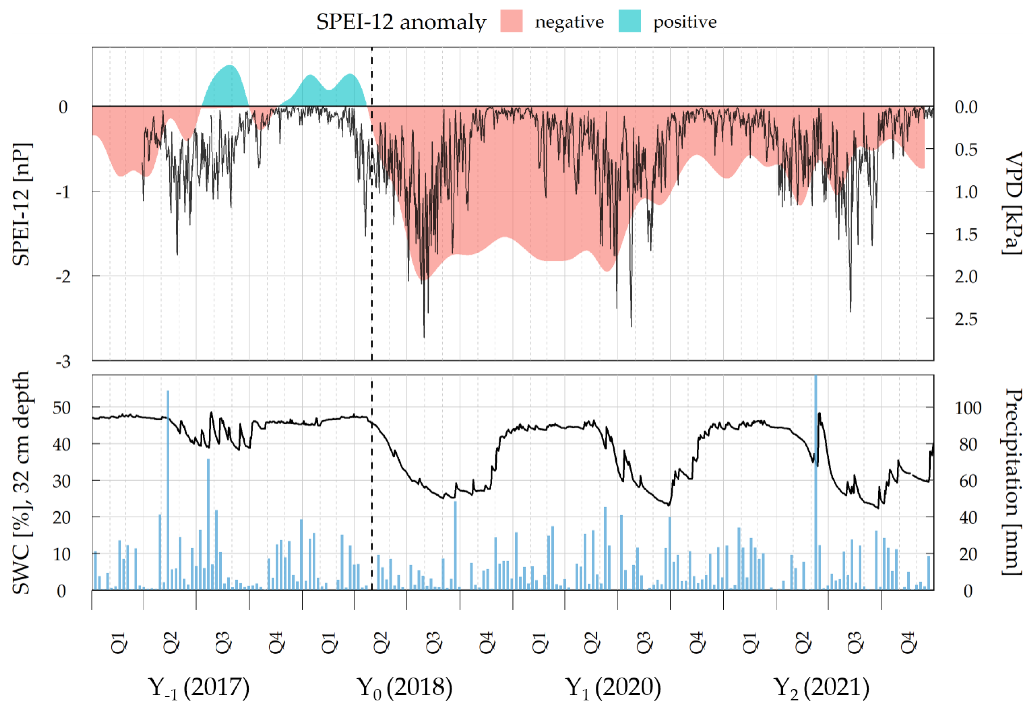
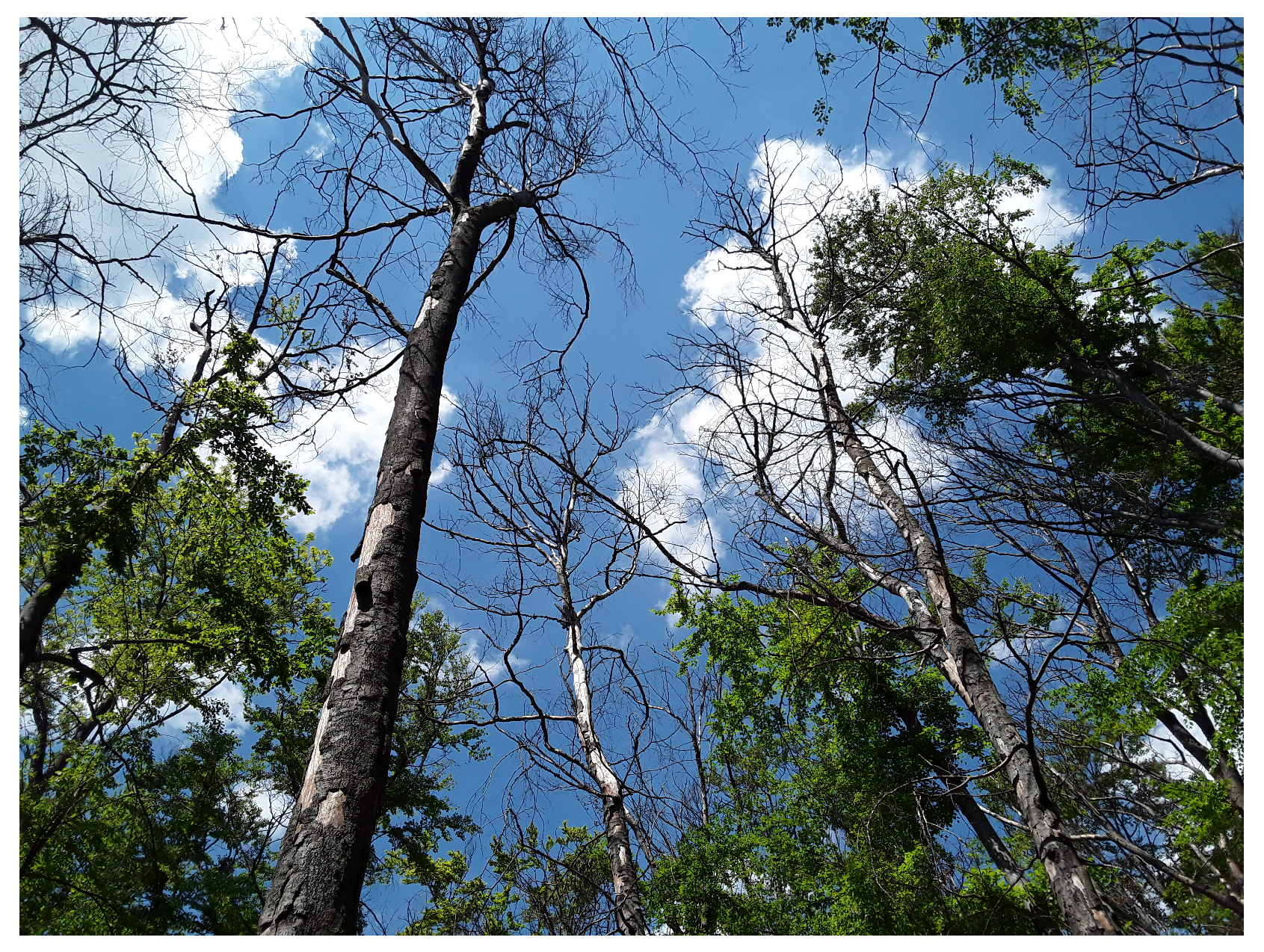
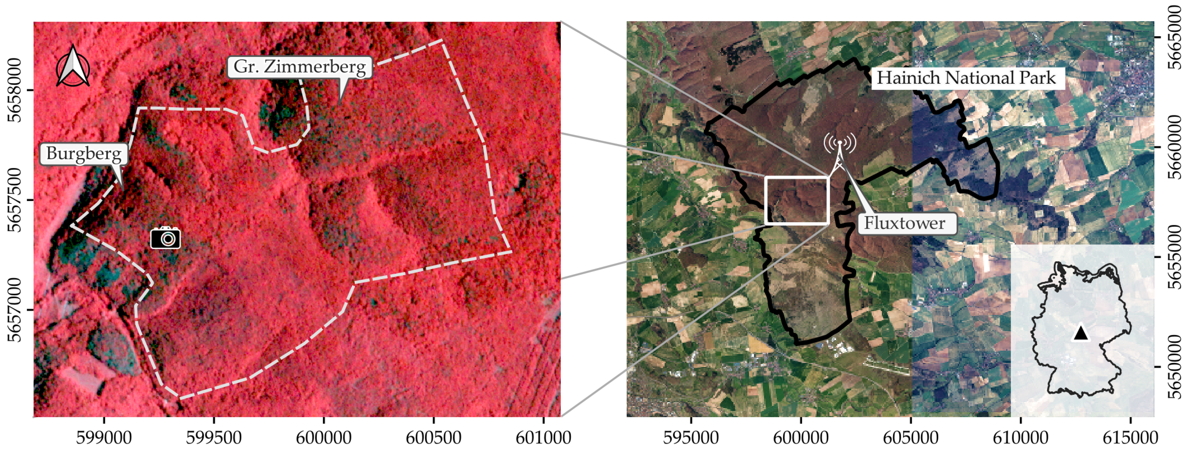
2.1. Study Site and Drought Impact

The study was conducted at Hainich National Park (HNP) in western Thuringia, Germany (lat: 10.4229 , lon: 51.0591 , mean elevation: 413 m a.s.l.), a mixed deciduous broadleaf forest dominated by European beech (Fagus sylvatica, 65%), ash (Fraxinus excelsior, 25%), maple (Acer pseudoplatanus, and Acer platanoides, combined 7%) with other deciduous species [47]. Due to its foundations in middle and upper Muschelkalk (shell limestones) and lower Keuper (claystone), the soils are relatively shallow, carbonated, and humus-rich with strong runoff (e.g., Rendzina, Regosol), with characteristics more pronounced on exposed slopes [48]. Thus, soils have limited storage capabilities and plant-available water rapidly declines under drought conditions.
This study refers to the successive droughts that took place in Central Europe in the years 2018–2020 [49]. Local meteorological data from an eddy covariance flux tower in the HNP indicate characteristics of an atmospheric drought and hydrological drought when compared to the 2000–2014 multi-year average [50]. Both, the anomaly of vapor pressure deficit (VPD) in 2018 of 0.302 kPa (+59%) and the extremely low SPEI drought index (description in Figure 1) indicate a strong negative water balance and atmospheric drought in these years (Figure 1). The strength of the hydrological drought was indicated by a soil water anomaly of −7.93% (−25%) in 2018, with storages not replenishing as of 2020. The climatological reference period of 2000–2014 was constrained by the measurement period of the Eddy covariance flux tower (DE-HAI), which was erected in 2000. We decided on tower data instead of a long-term record from the next meteorological station due to the large distance to the next station ( 10 km, Eisenach) and to account for DBF-specific energy fluxes at the site. We considered a 4-year period that started in 2017 and included the pre-event and the onset, as defined by the start of the SPEI anomaly, as of 4 April 2018, and the late stage of the drought (until 2020). The relative nomenclature used in this study ranged accordingly from Y 1 (2017) to Y 2 (2020). It is clear that data from such a narrow study period cannot capture long-term trends and is especially prone to uncertainty. Since the Sentinel-1A/B data record is limited, we restricted the study period to 4 years.
The multi-year drought has led to substantial tree canopy damage and dieback in vast areas in Central Europe, including Germany [12,53], and was also observed in the HNP [54] (Figure 2). We confined the study site to an area of plateaus in the western HNP (Figure 3) where increased crown damage could already be successfully delineated using drone and Sentinel-2 data [54,55].

2.2. Sentinel-1 Data Processing

Only SAR data (acquired in the early morning/predawn with a local overflight time of ~7:30 CEST (6:30 CET, 5:30 UTC)) were used. At predawn conditions, healthy plants establish a hydraulic equilibrium where the water potential between the soil and leaf tissue converges (tissues replenish) ([58], p. 556). Conversely, under the effect of droughts, leaf tissues cannot fully refill during the night [59]. In this sense, water-related measurements at predawn are expected to be the most reasonable proxy for hydraulic damage in the diurnal cycle, independent of photosynthetic activity in the daytime. To avoid geometric variability among orbits due to changes in incidence angles and look directions, only scenes with average sensor incidence angles θ of 36 over the study area were considered, corresponding to typical mid-range conditions (relative orbit 66). In total, 215 ESA Copernicus S-1 scenes with an average of 6-day revisit cycles (the same look direction, time of day, and sensor incidence angle) were processed for the period 2017–2020 [60] using single look complex (SLC) data (Figure 4). The SLC format is a precondition for performing a polarimetric eigenanalysis on the complex SAR signal and for temporal speckle filtering in radar (slant) geometry. The subsequent radar-specific processing steps were performed using the S-1 SNAP processor [61], accessed via the S-1 handler package ‘pyroSAR’ [62].
After applying the precise orbit file, all scenes were co-registered and a rolling arithmetical mean temporal speckle filter was applied pixel-wise to (1) the radiometric VV-VH intensities and (2) the complex 2-channel covariance matrix [ C 2 ] [63]. We leverage the frequent revisit time of the S-1 sensor by employing a temporal-only speckle filter to increase signal stability while keeping the maximum spatial resolution of 10 m × 10 m. Subsequently, [ C 2 ] was used for deriving H α . We iterated a filter set of the effective number of looks (ENL) { 3 , 7 , 13 , 19 } for assessing appropriate temporal filter sizes for the analysis. Despite the development of advanced time series filter methods, e.g., [64,65], filtering is usually not applicable for complex numbered data. A rolling mean operand was, therefore, used here for simplicity. Using default parameters, the radiometric data were normalized to radar brightness β 0 and terrain-flattened γ T 0 [66]. With the polarimetric data, the eigenproblem for [ C 2 ] was solved as described by Cloude [67] using custom implementations with python packages ‘numpy’ [68] and ‘numba’ [69]. Finally, all data were geocoded to a 10 × 10  m grid (UTM 32N, WGS 84) using a lidar-derived DTM and DSM, where the latter was low-pass filtered from 1 m to 5 m to avoid ambiguities due to rough canopy surfaces and crown gaps in forests [70]. With DTM and DSM representing the minimum (no forest, DTM) and maximum (canopy height, DSM) of possible geocoding reference planes, the range of DEM influences will be judged with their extrema. By using the lidar-derived DSM instead of the default DEM settings, the geolocations of canopies shifted from the DTM ground level to the prospected canopy level. We propose that this method enables an accurate overlay of the oblique acquisition geometry of SAR with nadir-looking instruments (S-2, UAV, lidar) for forest applications. This is necessary to locate single canopies onto the SAR imagery.
To assess the structural changes to the damaged trees, the additional polarimetric indices, i.e., cross-ratio (CR), radar vegetation index (RVI) [45], and Span were derived as follows:
C R = γ V V 0 / γ V H 0
R V I = 4 γ V H 0 γ V V 0 + γ V H 0
γ S p a n 0 = γ V V 0 + γ V H 0
where γ X X 0 represents either VV or VH calibrated and radiometric terrain corrected S-1 backscatter.

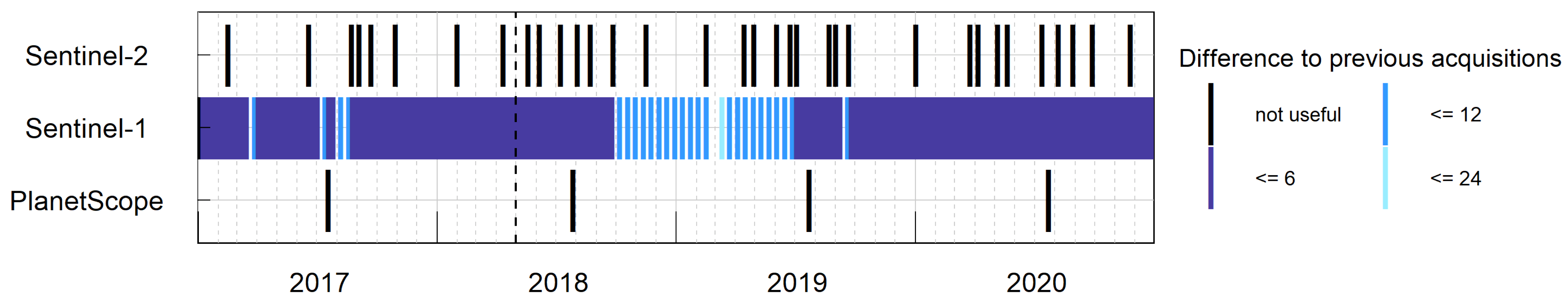
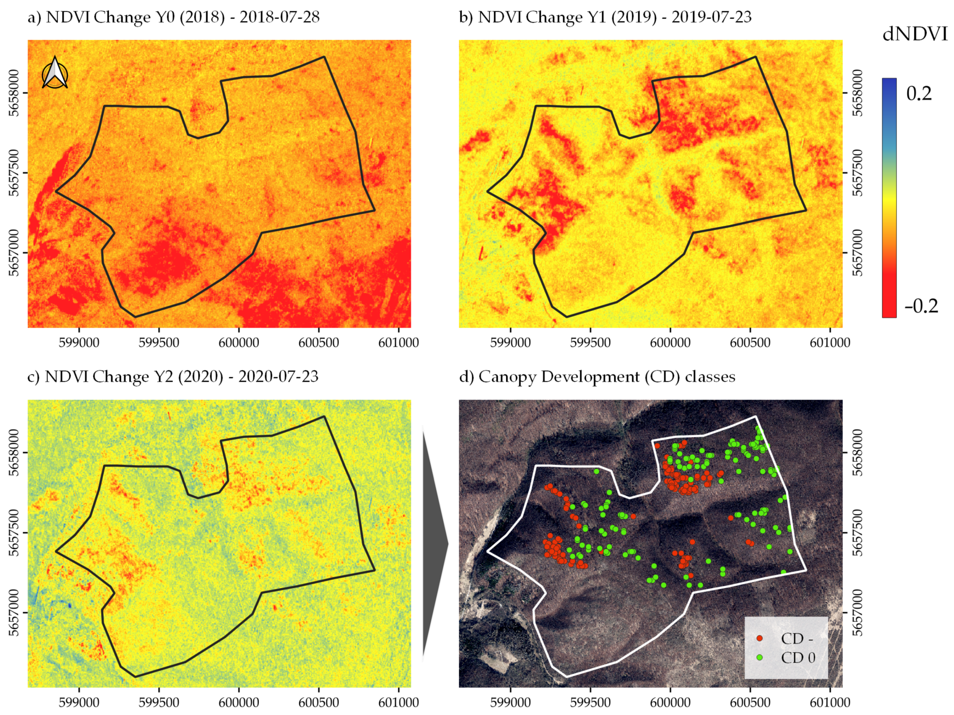
2.3. Optical Reference Data Processing

Optical remote sensing data are sensitive to DBF crown damage in the HNP [54] and are, therefore, used as indicators for canopy damage. First, very high resolution PlanetScope imagery is used to select damaged tree canopies bi-temporally before and after the drought to create an a-posteriori canopy damage sample set. Second, the multi-spectral ESA Copernicus Sentinel-2 (S-2) time series is used alongside S-1 to understand similarities and differences between SAR and optical forest drought signals.
The PlanetScope/Dove 4-band color-infrared data were retrieved at Level-3B as an analytic ortho-scene image product at 3 m of resolution [56]. Four cloud-free scenes in peak growing seasons were chosen to create NDVI-based vitality layers for each observation year (Figure 5). Pre-event N D V I Y 1 was defined as undamaged. NDVI change layers were created and defined as the differences of the respective year to pre-event conditions by Δ N D V I Y n Y 1 = N D V I Y n N D V I Y 1 . As radiometric inconsistencies between PlanetScope sensors reduced the quality of time series data [71], this study restricts its use to 1-sigma quantile classification in bi-temporal (pre- and post-droughts, Y 1 and Y 2 ) differences and visualizes damage patterns spatially. The a-posteriori Canopy Development (CD) tree sample sets were defined by:
CD −:Negative canopy development Δ N D V I < μ σ ,
(damaged, high mortality risk)
CD 0:Indifferent canopy development Δ N D V I < μ + σ a n d > μ σ ,
(undamaged or recovered, low mortality risk)
CD +:Positive canopy development Δ N D V I > μ + σ .
(re-greening, disregarded here)
where μ is the mean and σ is the standard deviation of the sample.
In the next step, the extracted CD sets were aligned to the S-1 data grid. After (bilinear) interpolation, these pixels were selected; they were members of either CD class (with 95% confidence interval). Due to the heterogeneity of the soils, forest age, height, stand density, and topography in the study area, we further employed a stratified sampling strategy to ensure that the samples were representative and classes had equal sizes. We filtered pixels with:
  • Canopy density > 80%;
  • Canopy height > 18 m;
  • Slope angle < 10 .
The thresholds were derived from assessing the environmental variable distributions and by local expert knowledge to minimize radar-relevant topographical effects (e.g., slopes) and to pursue relative forest homogeneity, especially by excluding non-mature forest patches (canopy height and density). As horizontal density ancillary data, the “Tree Cover Density” Copernicus high-resolution layer (2018) was used [72]. Slope angle and a canopy height model were derived from lidar DTM and DSM [70]. Finally, valley features were masked out. With a total of n = 146 samples per class, 292 10 × 10 pixels (2.92 ha) were selected (CD + is disregarded as re-growth patterns are not the primary focus of the study).
S-2 data were retrieved via the Microsoft Planetary Computer (MPC) cloud platform [73], which was processed to Level-2A bottom-of-the-atmosphere reflectances and terrain corrected with Planet DEM 30 by the Sen2Cor processor and MPC. The normalized difference vegetation index (NDVI) was calculated at 10 m native S-2 resolution using the bands 4 (red) and 8 (nir), after [74]. The normalized difference water index (NDWI) was favored for water assessments [75]; however, the NDVI was used here due to its damage sensitivity and the higher spatial resolution of S-2 at red/NIR bands (10 m) in comparison to the SWIR bands (20 m), which should match the chosen S-1 resolution. As clouds often only obscure parts of the imagery, no global cloud filter was applied and a total of 270 scenes were downloaded. Instead, we cut NDVI data at sampling sites where NDVI < 0.25, as those values were assumed to represent clouded pixels. Then, local maxima in the time series were detected using findpeaks from the ‘gsignal’ package [76] and R statistical software [77]. The 34 scenes left (Figure 4) were then linearly interpolated to all S-2 and S-1 acquisition dates. This way, more scenes in the S-2 time series could be kept, with stable intra-seasonal signals retained. Season thresholds in this study were tailored to the local forest and species composition by using the NDVI inflection points in the spring and fall based on pre-event data. Accordingly, the growing season and full foliage cover were assumed for DOY 130 (10 May)–280 (7 October).

2.4. Time Series Analysis and Statistical Methods

At first, time series data of SAR were used to evaluate intra-seasonal and inter-annual dynamics of the damaged CD− canopies. For this, we used class-wise averaged means of the damaged tree class for S-1 indices and S-2 NDVI. In this context, different temporal speckle filters were used and their suitability is discussed.
Secondly, the state and progress of damage in tree canopies were analyzed by calculating anomalies (differences) between CD− and CD 0 tree samples. The benefits of using spatial anomalies instead of temporal ones include (1) the leveling-out of short-term influences on the radar signal (e.g., rain interception) and (2) only damage-related features are visible. For a temporal anomaly calculus, we considered a reference period based on the data since the sensor launch (from 2015) was too low.
With speckle filtering, temporal autocorrelation was introduced in the S-1 time series. Thus, to avoid bloated statistics by auto-correlated sampling, only a single S-1 scene with the largest speckle filter size E N L = 19 was used for anomaly calculus and testing. For this, the most central scene (median of the acquisitions) in the peak leaf-on was used. Conversely, the NDVI time series did not carry out this autocorrelation. Hence, all NDVI peaks were used, as defined in Section 2.3.
Damage anomaly statistics were derived from differences in sample distributions of CD− and CD 0 as
Δ μ x y = μ x μ y
Δ σ x y = σ x 2 + σ y 2
where Δ μ x y and Δ σ x y are the mean and standard deviations (SD) of differences (anomalies) between population classes x (CD−) and y (CD 0). Due to unequal variances, Welch’s t-test [77] was calculated, hypothesizing that the sample means between CD− and CD 0, were equal. Note that normal distribution and random sampling of the population are assumed.
The extracted S-1 dual-pol indices were assessed toward their information content based on the correlation analysis. Due to the variety of polarimetric indices, we used a simple Spearman rank correlation and principal component analysis (PCA) method to judge if features add information to the analysis or are redundant. Here, a PCA is a useful tool to estimate feature distance. As many polarimetric indices have been designed for full-pol configurations, the usefulness of each index needs to be assessed for the use case prior to including them in a dual-pol analysis.

3. Results

3.1. Speckle Filtering and Geocoding of Dual-Pol SAR Time Series Data

Time series signal disturbance arises from, e.g., variations in wind speed (triggering tree swaying, rain interception, or freeze/thaw events). As these short-term phenomena affect tree status mapping, their propagation to the filtered time series is of concern. In this study, we found that, by increasing the filter size, the radiometric stability for γ S p a n 0 increased (Figure 6a,c) and SD decreased from ~2 dB to ~1.1 dB, for E N L = 3 and 19 , respectively. The interpretation of plant water status changes at damaged canopies was, therefore, only valid when stable environmental and phenological conditions could be assumed. For the sensitivity analysis, we restricted the data to leaf-on-only conditions (as represented by Y 1 NDVI seasonal inflection points). The remaining signal variances can, therefore, largely be explainable by changes in the plant water status.
The dual-pol entropy approaches a stable boundary with means of 0.7–0.8 and SD of ~0.08 at above E N L = 13 (Figure 6b). While Lee et al. [78] suggested an E N L = 49 for a reasonably unbiased spatial filter size for entropy, our data indicate a higher efficiency of speckle reduction in the temporal rather than in the spatial space. While the effect of combined spatiotemporal filtering has not been investigated, it holds large potential for harmonizing trade-offs. The annual trajectory of entropy suggests that scattering mechanisms simplify with the growing season and diversify again toward the fall.
Owning to the trade-off between high spatial (10 m pixels) and temporal resolution, we decided on E N L = 13 ( 80 days for our S-1 setup) for time series depictions. Yet, for the sensitivity analysis, seasonal averages are considered, represented by an E N L = 19 of the median scene of the summer season (see Section 2.4).
Concerning the correct detection of scattered mortality patterns, both lidar elevation models, DSM and DTM, have been used to geocode the SAR imagery. We found that the Δ γ S p a n 0 DSM backscatter dropped by ~0.5 dB in the late-stage drought ( Y 2 ) while Δ γ S p a n 0 DTM only decreased by ~0.2 dB. As CD class differentiation is only possible with DSM-geocoded data, we infer that tracking canopy changes (by an oblique SAR geometry at a very high spatial scale) requires an elevation model that reflects the top forest layer under study rather than ground topography. Further analyses are currently being performed and documented in [79].

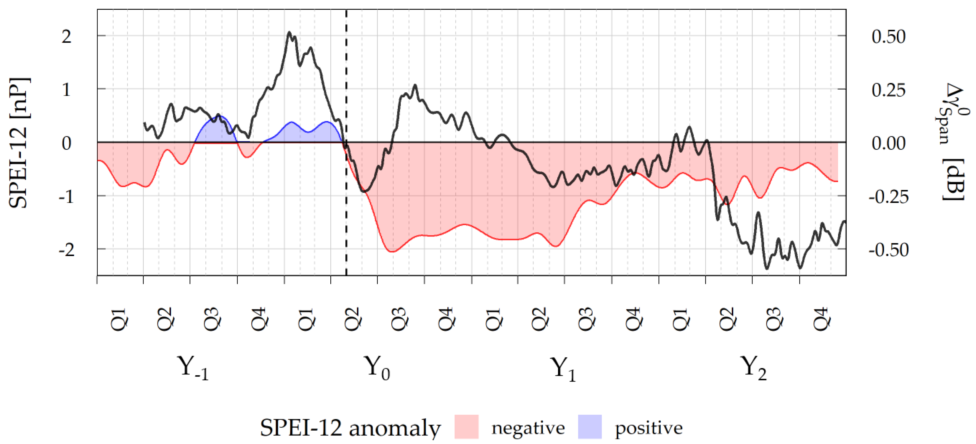
3.2. Temporal Signal of Drought-Stressed Broadleaf Forest

Describing the signal trajectory along the drought progression is vital to understanding anomalies induced by drought. Therefore, the time series of S-1 backscatter, CR, and S-2 NDVI at damaged tree canopies (CD−) is given in Figure 7. γ V V 0 and γ V H 0 have been found to decrease in the spring and rise again in the fall, complying with pre-drought conditions ( Y 1 ). The intra-annual changes in the plant water status can partly be disentangled in the SAR time series when carefully selecting phases of constant phenology. For example, while in Y 0 , a near-normal leaf development can be assumed (due to wet conditions in Y 1 ), the emerging drought conditions reduced vitality and chlorophyll activity from peak growing season onward (Figure 7d). Similarly, backscatter γ S p a n 0 in Y 0 decreased toward the fall (Figure 6a and Figure 7a). When assuming foliage to be fully developed and the tree structure to be constant, the observed early summer γ S p a n 0 decline can be attributed to water loss. The further decreasing γ S p a n 0 in the late summer, finally, mixes with structural decay in the canopies due to, e.g., premature leaf fall and wilting. Leaf-off γ V V 0 always remained below pre-drought conditions, indicating fundamental hydrological changes to the trees, as well as in the winter. S-2 NDVI has been found to decline in Y 0 toward the late summer, complying with European-wide observation of early wilting patterns [53,80]. Y 1 and Y 2 display strong vitality declines compared to the reference year.
The CR describes a magnitude with phenological phases, plateauing in summer, and increasing and decreasing in the spring and fall, respectively. In this sense, the slow slope of CR in the early summer Y 1 (DOY 150–200) can be related to delayed leaf development, only reaching its maximum (foliage) toward DOY ~250 (early September). NDVI-based vitality peaks earlier (DOY ~170) than CR in Y 1 , indicating that greenness and structural development do not necessarily co-evolve in drought-affected springs but show distinct developments. As signal delays or losses cannot be observed in Y 2 , CR eventually lacks clear interpretability in drought contexts.

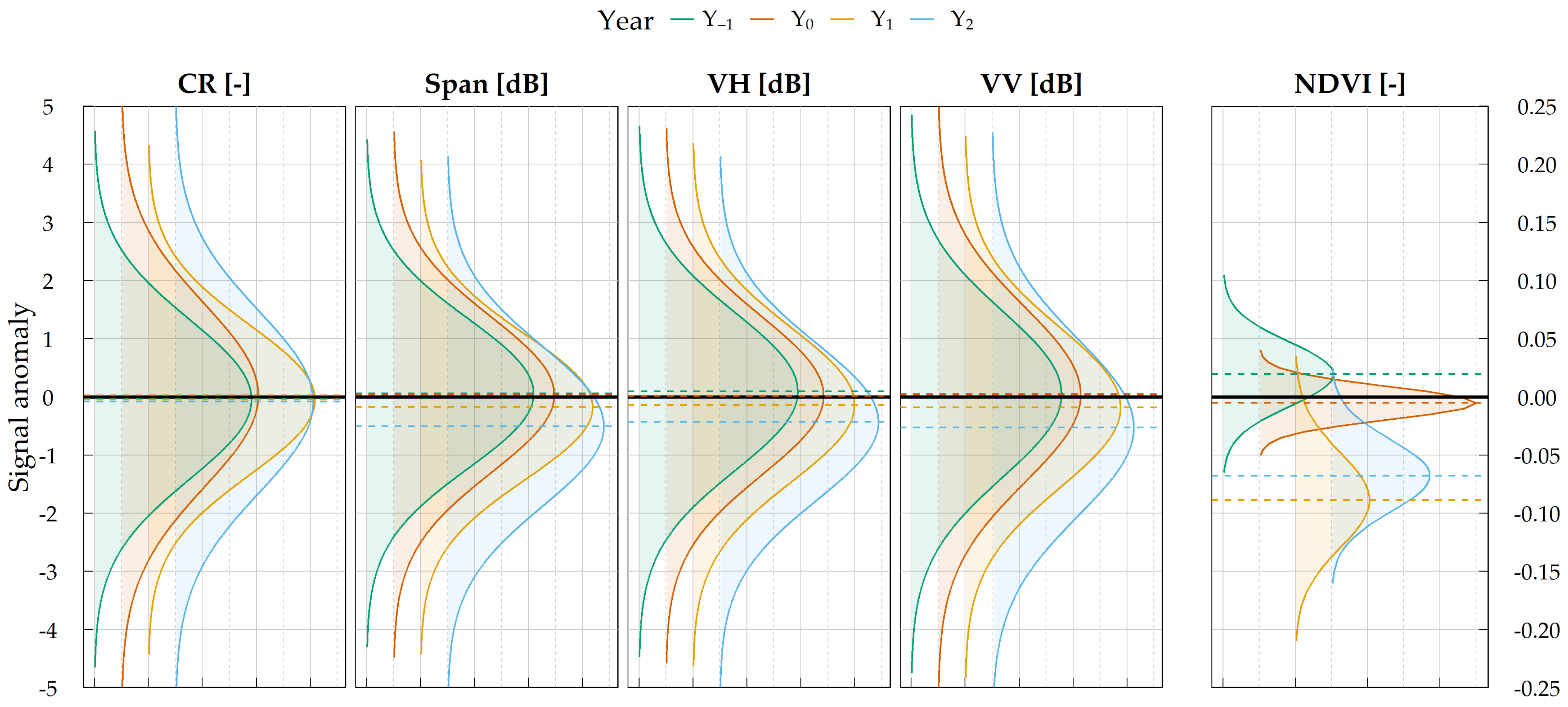
3.3. The Dual-Pol SAR Information Space

The dual-polarimetric capabilities of S-1 were statistically investigated using Spearman rank correlations and a PCA. All available data of classes CD− and CD 0 were used throughout all years. γ V V 0 and γ V H 0 were found to have a strong positive correlation of r = 0.72 (Figure 8a). In contrast, the CR was much less related to either SAR channel with r = 0.36 (VV) and r = −0.33 (VH). The correlations between CR and both eigen-based parameters were high, at −0.50 (entropy) and −0.43 (alpha), indicating a certain alignment of information content. As the dual-pol RVI essentially contains the same information content as CR, it will be disregarded in further analysis.
Results from the PCA are depicted in Figure 8. The cumulative variance reveals that the first three axes contain the main information directions in the data (Figure 8b). When looking at the relative contribution of the variables within axis 1, the dominant information contents of γ V V 0 and γ V H 0 (and γ S p a n 0 ) are visible (Figure 8c). The CR is orthogonally directed (axis 2) and similarly strong. Alpha is negatively correlated with CR, yet with a weaker signal, and the effect of entropy is low. We argue that the backscatter and CR carry most of the information content due to the orthogonality of CR to the backscatter, on the one hand, and the strong negative relation of alpha to CR and the marginal effects of entropy, on the other hand. Consequently, while γ S p a n 0 is used to represent S-1 radiometry, CR represents the polarimetric information content. The eigenvalues/contributions and the eigenvectors/angles do not directly imply strength in classifying damaged forests, they only hold information for deciding the most meaningful variables.

3.4. Sensitivity and Co-Evolution of SAR and Optical Data to Drought Impact

To test the sensitivity of S-1 γ S p a n 0 and CR regarding tree canopy damage under drought stress, the year-wise difference between CD− (damaged) and CD 0 (undamaged) tree samples were calculated. The S-1 backscatter of damaged trees declined moderately in Y 1 while significantly dropped in Y 2 (Figure 9), with average anomalies of −0.43 dB ± 1.36 (VH), −0.52 dB ± 1.52 (VV), and −0.50 dB ± 1.38 (Span) (Figure 10 and Table 1). Notably, Δ NDVI anomaly was largest in Y 1 (−0.089 ± 0.04) and decreased again in Y 2 (−0.068 ± 0.03), indicating that the trajectory between SAR and optical indices in late-stage drought damage diverged. It is clear from the data that the anomaly of NDVI is more certain than S-1-derived indices. However, as backscatter trends in Y 2 become significant, we can assert systematic changes to the scattering intensity of the C-band signal. The CD classes were defined on the basis of NDVI (PlanetScope-based) and, thus, changes to NDVI are self-evident.
The S-1 indices were compared regarding their discriminative strengths to drought damage. While Δ γ V V 0 had the largest anomaly and Δ γ V H 0 had the lowest SD among the backscatter data, Δ γ S p a n 0 had the highest t-value (4.42) in contrast to VV (4.17) and VH (3.80), indicating a higher ability for CD class differentiation. Although deviations between the signals are arguably small, we can still infer that γ S p a n 0 is statistically more stable than VV and VH for detecting drought effects in this context. Regarding Δ CR , anomalies remained statistically insignificant over the entire observation period. Furthermore, the statistical reliability of CR anomaly was hampered here due to very high errors with SD > 1.5 ( Y 2 ). Besides the potential for qualitatively interpreting changes to the seasonal cycle, CR does not show sensitivity to DBF forest droughts.
The differences between S-2 NDVI and S-1 Span signal trajectories in the drought aftermath allow for tracking multi-year damage recovery. Understanding the recovery patterns is useful in understanding the long-term implication of drought disturbances. On the NDVI/Span-plane (Figure 11), the trajectories of plant vitality versus microwave radiometry are given. Zero anomalies are expected for two cases: (1) No drought apparent, (2) drought influence for both populations (CD− and CD 0). While negative anomalies measure losses in vitality/chlorophyll activity or structural/water status for Δ NDVI and Δ γ S p a n 0 , respectively, positive anomalies can be caused by sampling errors or environmental unknowns. In contrast, Y 0 exhibits a strong drought effect for both sample populations (case 2). Only in late summer did Δ NDVI decrease, which may indicate drought damage accelerating in the following years. The effects of Δ γ S p a n 0 in Y 0 cannot be readily interpreted because of its large fluctuation (also visible in Figure 10). As all trees are damaged (see Figure 5), the signal could be explained by random variability in tree crown desiccation as seen by C-band SAR. While NDVI shows the largest anomaly ( −0.1) in Y 1 , γ S p a n 0 anomalies are moderate ( −0.18 dB). Finally, with Y 2 , two converse effects become visible: While anomalies in γ S p a n 0 further intensify, NDVI values regain, forming a hysteresis-like circular pattern.

4. Discussion

The sensitivity of Sentinel-1 SAR for capturing tree canopy damage and mortality patterns in Central European deciduous broadleaf forests was tested. We found that the S-1 Span was the best predictor of damage detection, and the largest backscatter anomaly was found in Y 2 of −0.5 dB ± 1.38, indicating coupled hydrostructural decay in drought-affected trees. Polarimetric indices, such as the widely used cross-ratio (CR), could not prove sensitivity to damage within our analysis. In light of the data fusion in forest monitoring, we found the SAR anomaly time series lagging behind NDVI in time by ca. one year after the onset of the drought, suggesting complementary information content of SAR to optical sensors.

4.1. The Role of SAR Processing in Drought Observations

The applied temporal-only speckle filter scheme reduces short-term disturbances in the S-1 signal time series. A filter size of E N L = 13 (~80 days) was shown to be a good trade-off between temporal decorrelation with phenology and biomass, and sufficient speckle reduction (Figure 6) for backscatter and polarimetric data. This enabled using credible S-1 maximum 10 m spatial pixel spacing, promoting as little spatial overlap as possible between damaged and non-damaged tree samples with their surroundings, acknowledging the heterogeneity of mortality patterns. However, with the long temporal correlation length introduced by filtering, weekly-to-monthly plant water status changes cannot be assessed independently of neighboring image acquisitions. Therefore, the signal can only be related to seasonal trends of desiccation and rehydration in canopy tissues. To increase the temporal resolution, combined spatiotemporal filtering strategies are, therefore, advised, especially in cases of high spatial homogeneity (e.g., large-scale bark beetle outbreaks). An 80-day averaging comes with the expense of ignoring short-term dynamics where outliers could corrupt the time series averaging, especially wind swaying [22], rain interception [81,82], and dew ([39], p. 508) [83,84]. To account for these factors, either threshold-based filters are found to be easy-to-use assets to gain more signal stability [82] or analytically based approaches (e.g., incorporating rain interception models [81]). Additionally, the full temporal resolution of S-1 data can be used by incorporating all relative orbit acquisitions to increase the observation density to up to 1.5 days. While this benefits the temporal coverage and allows similar ENL within a shorter time span, the incidence, azimuth angle, and diurnal variations (morning/afternoon overflight) will be introduced, which need to be further taken into account. For example, Weiß et al. [33] mitigated incidence angle influences by incorporating θ into microwave radiative transfer models.

4.2. Detecting Hydrostructural Changes to C-Band SAR in a Damage Forest Canopy

Drought conditions reduce canopy water content and limit tree leaf development and foliage duration (e.g., due to early leaf fall). Since S-1 summer anomalies of γ S p a n 0 correlate with tree canopy damage, coupled hydrostructural declines in those trees are suggested (see Figure 10). We hypothesize that the observed backscatter decline can be related to (1) losses in water content in damaged plant components, e.g., due to disturbed hydraulic uptake and (2) the decline in the number of vegetation scatterers due to losses in the tree structure (leaf and, eventually, branch loss), especially in the late stage of mortality. Furthermore, since Walthert et al. [59] showed that xylem damage occurs before leaf loss in damaged mature beeches, changes in growing season backscatter may be related to mortality-induced plant water status changes instead of changes to leaf biomass, i.e., a decline in plant water content and uptake. To validate the interpretation of SAR signal losses, the link to in situ tree physiology is essential. When relating the thresholds of individual water stress to SAR, we gain the unique ability to understand plant water status and, finally, mortality in more spatial and temporal details.
As we have seen, the backscatter decline in Y 0 can be interpreted as the loss of canopy water content when assuming the biomass is constant (see Figure 7). The assumption is, however, violated with (early) leaf loss as the phenological boundary. With leaf fall, signal attenuation from an undamaged canopy diminishes, and contributions of the branch, stem, and soil moisture simultaneously increase [41]. For damaged trees, the winter backscatter is found to be strongly reduced (Figure 7a). The winter/leaf-off backscatter in an undamaged forest usually exceeds values measured in summer/leaf-on months. Our data suggest contrasts with normal behaviors found in the pre-drought period Y 1 and literature (see [85]). The tree structure decline in the backscatter relates to the low water content in the desiccated damaged tissues under leaf-off conditions. Its correlation with tree desiccation is, however, conceivable. As the soil moisture of the upper layers is not variable in the winter—which may not be accurate for deeper hydrological layers—changes in soil moisture cannot explain the low winter backscatter alone. To test this, detailed knowledge about the leaf-off water content of damaged and undamaged trees, the allocation of scattered contributions to specific plant layers, and quantifying the soil contribution and soil water content are necessary. Further, physically modeling the backscatter as a function of phenology can broaden our understanding of the DBF backscatter in the winter; a crucial asset for interpreting S-1 time series data in this biome.
A promising approach exploits the separation of plant water status, phenology, and biomass dynamics when growth is absent, e.g., at a diurnal level. Here, diurnal measurements yielded encouraging results for quantifying water stress [13,15,86,87]. The suitability of S-1 for entering the diurnal observation domain is, however, far-fetched due to the long time lags between morning and evening acquisitions (3–6 days). Approaches for forests, while successfully used for water stress detection in agricultural areas [88], need to be developed. As mentioned earlier, using different S-1 orbits further introduces variabilities in incidence and azimuth angles that need to be considered.

4.3. Potential of S-1 Polarimetry for Detecting Changes in Scattering Mechanisms

Changes in scattering mechanisms in drought-damaged tree canopies were expected to shift the polarimetric SAR signatures from volume scattering to simpler scattering mechanisms after the onset of drought. Dual-polarimetric S-1 variables (CR, RVI, entropy, alpha) showed sensitivity to the seasonal dynamics of deciduous trees (see entropy in Figure 6b and CR in Figure 7c) and, thus, covaries with phenology. This supports the interpretation that CR is sensitive to the presence and absence of leaves and, thus, reacts to substantial changes to the tree structure [32,43,85]. Still, changes in CR with crown damage could not be observed in our study. In contrast to the findings in [35,36], which used CR as a proxy for defoliation, similar signs of signal loss were not significant in our data during the growing season (see CR anomaly in Table 1). We conclude that CR helps to interpret phenology in DBF forests. However, a clear role in the structural decay of CR under drought stress needs further research and detailed knowledge about the canopy structure and phenology.
Due to the high-entropy regime (H > 0.6), ambiguities in scattering mechanisms are common problems for forests, especially at the C-band, impeding the successful retrieval of polarimetric information. Our experimental results comply with the simulations by Ji and Wu [89], showing that co-cross (VV-VH) polarization combinations could not correctly identify the canonical scattering mechanisms compared to full-polarimetric or co-pol dual-polarimetric setups (VV-HH). Still, a careful 3D separation of backscatter contributions from tree compartments (twigs, branches, stems) and the ground would strongly facilitate interpreting the detected annual cycle of the dual-pol entropy. Studying forests with multi-temporal, fully polarimetric SAR systems would help researchers understand microwave scattering in forests under changing phenology.
CR and Span were statistically found to be the most independent in the PCA based on the orthogonality of information content. As either variable can be directly calculated from VV and VH intensities (e.g., from ESAs GRD product), one can reconsider sparring the computationally demanding processing of complex-numbered SLCs and the eigenanalysis in favor of the simpler CR and Span. The high magnitudes and low errors found in Span indicate a slight improvement over using VV or VH channels alone in terms of more stable anomaly detection. Therefore, we suggest its use for mortality assessment and, more generally, for applications focusing on SAR radiometry.

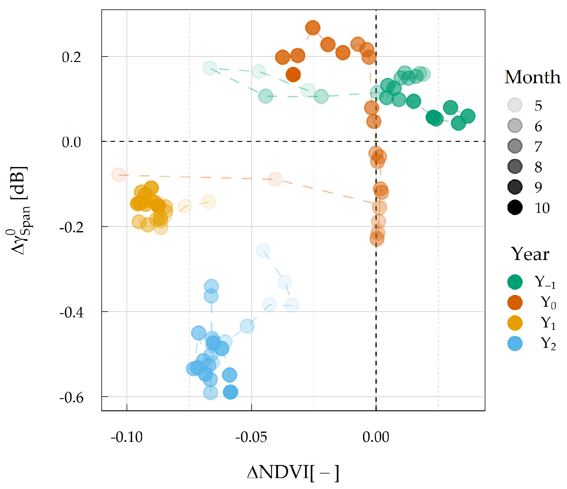
4.4. Time-Lagged Damage Patterns in the NDVI/Span-Plane

An NDVI/Span-plane was introduced that reveals the lagged signal anomaly in the backscatter against optically-derived vitality indices along the impact and recovery phases of the drought. If trees desiccate and die, water content and leaf/twig loss will lead to long-term structural decay, as captured by the S-1 Span. At the same time, photosynthetic activity showed tendencies for recovery ( Y 2 ). Thus, a time-lagged correlation between Δ NDVI and Δ γ S p a n 0 is implied, highlighting the different aspects and capabilities of optical and SAR sensors for detecting damage patterns and, ultimately mortality. While this approach is not suitable for characterizing drought sequences, it can be the basis for the multi-sensor remote sensing of disturbance ecology.
The NDVI/Span-plane can help researchers understand coupled photosynthetic and hydrostructural decay in the time domain for studying the damage and recovery of forests. In this sense, a forest would return to its Cartesian origin once it recovers from drought disturbance. The position of the hysteresis would then characterize its drought impact and recovery stage.
The recovery of Δ NDVI in Y 2 suggests an increase of greenness and vegetation vitality at damaged tree sites (CD−) at the late stages of droughts. A possible explanation is the development of undergrowth vegetation and pioneering plants underneath desiccated/dead trees. Moreover, if droughts are not lethal for individual trees, the partial regrowth of compartments may occur, or mixed pixels containing adjacent recovered or undamaged individuals may affect NDVI. Positive values of anomalies between CD− and CD 0 are found in Y 1 and Y 0 , indicating inconsistencies in the sample set. The data cannot explain positive values when assuming that the samples are drawn from the same tree population and damage leads to a decline in the backscatter and NDVI. Unknown variations in the population can play roles, including demography (age, species), forest structure (vertical and horizontal distribution), topography (e.g., aspect), soil/geology (e.g., soil composition, rock formations, runoff scheme), and variables that go beyond the initial sampling scheme (NDVI threshold, slope, canopy height, tree cover density).

5. Conclusions

Our results suggest that the Sentinel-1 backscatter can track the evolution of tree canopy damage at very high spatial (10 m × 10 m) and moderate temporal (~80 days) scales in a temperate deciduous broadleaf forest. S-1 polarimetric indices did not show the significant separation of damaged and undamaged trees, which was partly attributed to the high entropy scattering in the forests and the dual-pol sensor properties. The S-1 Span showed the best capability for assessing tree canopy damage. If considering periods of constant biomass, such as the peak growing season, backscatter anomalies can be carefully related to the plant water status. However, additional data on the plant water status are necessary to validate this conclusion. With the SAR anomaly time series lagging behind optically derived vitality indices in time by ca. one year, the long-term structural decay in the aftermath of drought years can be monitored. Further, with the help of the circular pattern in a Span/NDVI observation space, a tool for quantifying forest decline and recovery stages is provided. Based on the introduced methodology, a SAR-based or SAR-enhanced monitoring tool for observing long-term forest drought damage and its application in other broadleaf is conceivable. For mapping damage, integrating the sensors would enable the unique benefits of each frequency domain for retrieving mortality-relevant forest parameters, by, e.g., combining NDVI-based vitality and phenology information with SAR-based plant water status and structure.
Since speckle variance strongly decreases confidence in anomaly detection and still hinders out-of-the-box mapping with our data, new methods for estimating speckle patterns in time should be applied when working at very high spatial resolutions. Extending the reference dataset to other forest types and areas of known tree mortality would build the basis for SAR damage assessment outside of this local experiment. Other central unknowns comprise the discrimination of plant water status from meteorological factors, tree structure, and phenology, and understanding the backscatter contributions from different vegetation layers in the C-band, primarily under drought stress. At this point, the data gap in a tree’s physiological measurements for retrieved remote sensing forest hydrological parameters strongly limits advancing toward forest stress mapping. Shortcomings in the interpretability of SAR signals should further motivate research to analytically model microwave scattering along phenological and diurnal phases to retrieve the stand-level water status directly from microwave measurements. While recent advances in VWC modeling based on the transmission parameter VOD show promising results for linking water status and drought stress to microwave measurements at a coarse spatial resolution, the transfer to active SAR systems will be a crucial advantage for high-resolution mapping of forest health and tree mortality.

Author Contributions

Conceptualization, K.S., T.J., C.D., M.U. (Marcel Urban), and M.U. (Mikhail Urbazaev); methodology, K.S., T.J., C.D., and M.Z.; formal analysis, K.S.; software, K.S.; writing—original draft preparation, K.S., T.J., and C.D.; writing—review and editing, T.J., C.D., M.U. (Marcel Urban), M.U. (Mikhail Urbazaev), S.H., H.H., and C.S.; visualization, K.S.; supervision, T.J., C.D., and C.S.; project administration, C.D.; funding acquisition, C.S. All authors have read and agreed to the published version of the manuscript.

Funding

We acknowledge support by the German Research Foundation Projekt-Nr. 512648189 and the Open Access Publication Fund of the Thüringer Universitäts- und Landesbibliothek Jena.

Data Availability Statement

Not applicable.

Acknowledgments

The authors want to express gratitude for Manfred Großmann (Nationalpark Hainich) for sharing crucial knowledge about the 2018/2019 drought impact on beech trees at Hainich National Park. The authors like to further thank Anne Klosterhalfen (University Göttingen) for her support with pre-processed FLUXNET data of the Hainich Eddy Covariance Flux Tower.

Conflicts of Interest

The authors declare no conflict of interest.

References

  1. Masson-Delmotte, V.; Zhai, P.; Pirani, A.; Connors, S.; Péan, C.; Berger, S.; Caud, N.; Chen, Y.; Goldfarb, L.; Gomis, M.I.; et al. (Eds.) Climate Change 2021: The Physical Science Basis. Contribution of Working Group I to the SixthAssessment Report of the Intergovernmental Panel on Climate Change; Cambridge University Press: Cambridge, UK, 2021; in press. [Google Scholar]
  2. Touma, D.; Ashfaq, M.; Nayak, M.A.; Kao, S.C.; Diffenbaugh, N.S. A multi-model and multi-index evaluation of drought characteristics in the 21st century. J. Hydrol. 2015, 526, 196–207. [Google Scholar] [CrossRef]
  3. Dai, A. Increasing drought under global warming in observations and models. Nat. Clim. Chang. 2012, 3, 52–58. [Google Scholar] [CrossRef]
  4. Hammond, W.M.; Williams, A.P.; Abatzoglou, J.T.; Adams, H.D.; Klein, T.; López, R.; Sáenz-Romero, C.; Hartmann, H.; Breshears, D.D.; Allen, C.D. Global field observations of tree die-off reveal hotter-drought fingerprint for Earth’s forests. Nat. Commun. 2022, 13, 1761. [Google Scholar] [CrossRef] [PubMed]
  5. Trumbore, S.; Brando, P.; Hartmann, H. Forest health and global change. Science 2015, 349, 814–818. [Google Scholar] [CrossRef]
  6. Hartmann, H.; Schuldt, B.; Sanders, T.G.M.; Macinnis-Ng, C.; Boehmer, H.J.; Allen, C.D.; Bolte, A.; Crowther, T.W.; Hansen, M.C.; Medlyn, B.E.; et al. Monitoring global tree mortality patterns and trends. Report from the VW symposium ‘Crossing scales and disciplines to identify global trends of tree mortality as indicators of forest health’. New Phytol. 2018, 217, 984–987. [Google Scholar] [CrossRef]
  7. Hunt, E.R.; Rock, B.N.; Nobel, P.S. Measurement of leaf relative water content by infrared reflectance. Remote Sens. Environ. 1987, 22, 429–435. [Google Scholar] [CrossRef]
  8. Ceccato, P.; Flasse, S.; Tarantola, S.; Jacquemoud, S.; Grégoire, J.M. Detecting vegetation leaf water content using reflectance in the optical domain. Remote Sens. Environ. 2001, 77, 22–33. [Google Scholar] [CrossRef]
  9. Farella, M.M.; Fisher, J.B.; Jiao, W.; Key, K.B.; Barnes, M.L. Thermal remote sensing for plant ecology from leaf to globe. J. Ecol. 2022, 110, 1996–2014. [Google Scholar] [CrossRef]
  10. West, H.; Quinn, N.; Horswell, M. Remote sensing for drought monitoring impact assessment: Progress, past challenges and future opportunities. Remote Sens. Environ. 2019, 232, 111291. [Google Scholar] [CrossRef]
  11. Huang, C.; Anderegg, W.R.; Asner, G.P. Remote sensing of forest die-off in the Anthropocene: From plant ecophysiology to canopy structure. Remote Sens. Environ. 2019, 231, 111233. [Google Scholar] [CrossRef]
  12. Thonfeld, F.; Gessner, U.; Holzwarth, S.; Kriese, J.; da Ponte, E.; Huth, J.; Kuenzer, C. A First Assessment of Canopy Cover Loss in Germany’s Forests after the 2018–2020 Drought Years. Remote Sens. 2022, 14, 562. [Google Scholar] [CrossRef]
  13. Konings, A.G.; Saatchi, S.S.; Frankenberg, C.; Keller, M.; Leshyk, V.; Anderegg, W.R.L.; Humphrey, V.; Matheny, A.M.; Trugman, A.; Sack, L.; et al. Detecting forest response to droughts with global observations of vegetation water content. Glob. Chang. Biol. 2021, 27, 6005–6024. [Google Scholar] [CrossRef]
  14. Steele-Dunne, S.C.; McNairn, H.; Monsivais-Huertero, A.; Judge, J.; Liu, P.W.; Papathanassiou, K. Radar Remote Sensing of Agricultural Canopies: A Review. IEEE J. Sel. Top. Appl. Earth Obs. Remote Sens. 2017, 10, 2249–2273. [Google Scholar] [CrossRef]
  15. Frolking, S.; Milliman, T.; Palace, M.; Wisser, D.; Lammers, R.; Fahnestock, M. Tropical forest backscatter anomaly evident in SeaWinds scatterometer morning overpass data during 2005 drought in Amazonia. Remote Sens. Environ. 2011, 115, 897–907. [Google Scholar] [CrossRef]
  16. Friesen, J.; Steele-Dunne, S.C.; van de Giesen, N. Diurnal Differences in Global ERS Scatterometer Backscatter Observations of the Land Surface. IEEE Trans. Geosci. Remote Sens. 2012, 50, 2595–2602. [Google Scholar] [CrossRef]
  17. Frappart, F.; Wigneron, J.P.; Li, X.; Liu, X.; Al-Yaari, A.; Fan, L.; Wang, M.; Moisy, C.; Masson, E.L.; Lafkih, Z.A.; et al. Global Monitoring of the Vegetation Dynamics from the Vegetation Optical Depth (VOD): A Review. Remote Sens. 2020, 12, 2915. [Google Scholar] [CrossRef]
  18. Konings, A.G.; Holtzman, N.M.; Rao, K.; Xu, L.; Saatchi, S.S. Interannual Variations of Vegetation Optical Depth are Due to Both Water Stress and Biomass Changes. Geophys. Res. Lett. 2021, 48, e2021GL095267. [Google Scholar] [CrossRef]
  19. Rao, K.; Anderegg, W.R.; Sala, A.; Martínez-Vilalta, J.; Konings, A.G. Satellite-based vegetation optical depth as an indicator of drought-driven tree mortality. Remote Sens. Environ. 2019, 227, 125–136. [Google Scholar] [CrossRef]
  20. Jagdhuber, T.; Jonard, F.; Fluhrer, A.; Chaparro, D.; Baur, M.J.; Meyer, T.; Piles, M. Toward estimation of seasonal water dynamics of winter wheat from ground-based L-band radiometry: A concept study. Biogeosciences 2022, 19, 2273–2294. [Google Scholar] [CrossRef]
  21. Holtzman, N.M.; Anderegg, L.D.L.; Kraatz, S.; Mavrovic, A.; Sonnentag, O.; Pappas, C.; Cosh, M.H.; Langlois, A.; Lakhankar, T.; Tesser, D.; et al. L-band vegetation optical depth as an indicator of plant water potential in a temperate deciduous forest stand. Biogeosciences 2021, 18, 739–753. [Google Scholar] [CrossRef]
  22. Monteith, A.R.; Ulander, L.M.H. Temporal Characteristics of P-Band Tomographic Radar Backscatter of a Boreal Forest. IEEE J. Sel. Top. Appl. Earth Obs. Remote Sens. 2021, 14, 1967–1984. [Google Scholar] [CrossRef]
  23. Vermunt, P.C.; Khabbazan, S.; Steele-Dunne, S.C.; Judge, J.; Monsivais-Huertero, A.; Guerriero, L.; Liu, P.W. Response of Subdaily L-Band Backscatter to Internal and Surface Canopy Water Dynamics. IEEE Trans. Geosci. Remote Sens. 2021, 59, 7322–7337. [Google Scholar] [CrossRef]
  24. Garrity, S.R.; Allen, C.D.; Brumby, S.P.; Gangodagamage, C.; McDowell, N.G.; Cai, D.M. Quantifying tree mortality in a mixed species woodland using multitemporal high spatial resolution satellite imagery. Remote Sens. Environ. 2013, 129, 54–65. [Google Scholar] [CrossRef]
  25. Torres, R.; Snoeij, P.; Geudtner, D.; Bibby, D.; Davidson, M.; Attema, E.; Potin, P.; Rommen, B.; Floury, N.; Brown, M.; et al. GMES Sentinel-1 mission. Remote Sens. Environ. 2012, 120, 9–24. [Google Scholar] [CrossRef]
  26. Hoekman, D. Measurements of the backscatter and attenuation properties of forest stands at X-, C- and L-band. Remote Sens. Environ. 1987, 23, 397–416. [Google Scholar] [CrossRef]
  27. Kaiser, P.; Buddenbaum, H.; Nink, S.; Hill, J. Potential of Sentinel-1 Data for Spatially and Temporally High-Resolution Detection of Drought Affected Forest Stands. Forests 2022, 13, 2148. [Google Scholar] [CrossRef]
  28. Dostálová, A.; Lang, M.; Ivanovs, J.; Waser, L.T.; Wagner, W. European Wide Forest Classification Based on Sentinel-1 Data. Remote Sens. 2021, 13, 337. [Google Scholar] [CrossRef]
  29. Reiche, J.; Mullissa, A.; Slagter, B.; Gou, Y.; Tsendbazar, N.E.; Odongo-Braun, C.; Vollrath, A.; Weisse, M.J.; Stolle, F.; Pickens, A.; et al. Forest disturbance alerts for the Congo Basin using Sentinel-1. Environ. Res. Lett. 2021, 16, 024005. [Google Scholar] [CrossRef]
  30. Ygorra, B.; Frappart, F.; Wigneron, J.; Moisy, C.; Catry, T.; Baup, F.; Hamunyela, E.; Riazanoff, S. Monitoring loss of tropical forest cover from Sentinel-1 time-series: A CuSum-based approach. Int. J. Appl. Earth Obs. Geoinf. 2021, 103, 102532. [Google Scholar] [CrossRef]
  31. Rüetschi, M.; Small, D.; Waser, L. Rapid Detection of Windthrows Using Sentinel-1 C-Band SAR Data. Remote Sens. 2019, 11, 115. [Google Scholar] [CrossRef]
  32. Soudani, K.; Delpierre, N.; Berveiller, D.; Hmimina, G.; Vincent, G.; Morfin, A.; Dufrêne, É. Potential of C-band Synthetic Aperture Radar Sentinel-1 time-series for the monitoring of phenological cycles in a deciduous forest. Int. J. Appl. Earth Obs. Geoinf. 2021, 104, 102505. [Google Scholar] [CrossRef]
  33. Weiß, T.; Ramsauer, T.; Jagdhuber, T.; Löw, A.; Marzahn, P. Sentinel-1 Backscatter Analysis and Radiative Transfer Modeling of Dense Winter Wheat Time Series. Remote Sens. 2021, 13, 2320. [Google Scholar] [CrossRef]
  34. Rao, K.; Williams, A.P.; Flefil, J.F.; Konings, A.G. SAR-enhanced mapping of live fuel moisture content. Remote Sens. Environ. 2020, 245, 111797. [Google Scholar] [CrossRef]
  35. Bae, S.; Müller, J.; Förster, B.; Hilmers, T.; Hochrein, S.; Jacobs, M.; Leroy, B.M.L.; Pretzsch, H.; Weisser, W.W.; Mitesser, O. Tracking the temporal dynamics of insect defoliation by high-resolution radar satellite data. Methods Ecol. Evol. 2021, 13, 121–132. [Google Scholar] [CrossRef]
  36. Hollaus, M.; Vreugdenhil, M. Radar Satellite Imagery for Detecting Bark Beetle Outbreaks in Forests. Curr. For. Rep. 2019, 5, 240–250. [Google Scholar] [CrossRef]
  37. Vreugdenhil, M.; Wagner, W.; Bauer-Marschallinger, B.; Pfeil, I.; Teubner, I.; Rüdiger, C.; Strauss, P. Sensitivity of Sentinel-1 Backscatter to Vegetation Dynamics: An Austrian Case Study. Remote Sens. 2018, 10, 1396. [Google Scholar] [CrossRef]
  38. Mandal, D.; Kumar, V.; Ratha, D.; Dey, S.; Bhattacharya, A.; Lopez-Sanchez, J.M.; McNairn, H.; Rao, Y.S. Dual polarimetric radar vegetation index for crop growth monitoring using Sentinel-1 SAR data. Remote Sens. Environ. 2020, 247, 111954. [Google Scholar] [CrossRef]
  39. Ulaby, F.T.; Long, D.G. Microwave Radar and Radiometric Remote Sensing; Artech House: Norwood, MA, USA, 2015. [Google Scholar]
  40. Proisy, C.; Mougin, E.; Dufrene, E.; Dantec, V.L. Monitoring seasonal changes of a mixed temperate forest using ERS SAR observations. IEEE Trans. Geosci. Remote Sens. 2000, 38, 540–552. [Google Scholar] [CrossRef]
  41. Steele-Dunne, S.C.; Friesen, J.; van de Giesen, N. Using Diurnal Variation in Backscatter to Detect Vegetation Water Stress. IEEE Trans. Geosci. Remote Sens. 2012, 50, 2618–2629. [Google Scholar] [CrossRef]
  42. Ulaby, F.T.; Sarabandi, K.; McDonald, K.; Whitt, M.; Dobson, C.M. Michigan microwave canopy scattering model. Int. J. Remote Sens. 1990, 11, 1223–1253. [Google Scholar] [CrossRef]
  43. Frison, P.L.; Fruneau, B.; Kmiha, S.; Soudani, K.; Dufrêne, E.; Toan, T.L.; Koleck, T.; Villard, L.; Mougin, E.; Rudant, J.P. Potential of Sentinel-1 Data for Monitoring Temperate Mixed Forest Phenology. Remote Sens. 2018, 10, 2049. [Google Scholar] [CrossRef]
  44. Dubois, C.; Mueller, M.M.; Pathe, C.; Jagdhuber, T.; Cremer, F.; Thiel, C.; Schmullius, C. Characterization of land cover seasonality in Sentinel-1 time series data. ISPRS Ann. Photogramm. Remote. Sens. Spat. Inf. Sci. 2020, V-3-2020, 97–104. [Google Scholar] [CrossRef]
  45. Trudel, M.; Charbonneau, F.; Leconte, R. Using RADARSAT-2 polarimetric and ENVISAT-ASAR dual-polarization data for estimating soil moisture over agricultural fields. Can. J. Remote Sens. 2012, 38, 514–527. [Google Scholar] [CrossRef]
  46. Lee, J.S.; Pottier, E. Polarimetric Radar Imaging: From Basics to Applications, 1st ed.; CRC Press: Boca Raton, FL, USA, 2009. [Google Scholar]
  47. Kutsch, W.L.; Persson, T.; Schrumpf, M.; Moyano, F.E.; Mund, M.; Andersson, S.; Schulze, E.D. Heterotrophic soil respiration and soil carbon dynamics in the deciduous Hainich forest obtained by three approaches. Biogeochemistry 2010, 100, 167–183. [Google Scholar] [CrossRef]
  48. Küsel, K.; Totsche, K.U.; Trumbore, S.E.; Lehmann, R.; Steinhäuser, C.; Herrmann, M. How Deep Can Surface Signals Be Traced in the Critical Zone? Merging Biodiversity with Biogeochemistry Research in a Central German Muschelkalk Landscape. Front. Earth Sci. 2016, 4, 32. [Google Scholar] [CrossRef]
  49. Buras, A.; Rammig, A.; Zang, C.S. Quantifying impacts of the 2018 drought on European ecosystems in comparison to 2003. Biogeosciences 2020, 17, 1655–1672. [Google Scholar] [CrossRef]
  50. Knohl, A.; Siebicke, L.; Tiedemann, F.; Kolle, O.; ICOS Ecosystem Thematic Centre. Drought-2018 Ecosystem Eddy Covariance Flux Product from Hainich. 2020. Available online: https://meta.icos-cp.eu/objects/G8hl-qva-o-MVevf_5D_e1-0 (accessed on 1 May 2021).
  51. Vicente-Serrano, S.M.; Beguería, S.; López-Moreno, J.I. A Multiscalar Drought Index Sensitive to Global Warming: The Standardized Precipitation Evapotranspiration Index. J. Clim. 2010, 23, 1696–1718. [Google Scholar] [CrossRef]
  52. Monteith, J.; Unsworth, M. Principles of Environmental Physics, 3rd ed.; Academic Press: Cambridge, MA, USA, 2007; p. 408. [Google Scholar]
  53. Schuldt, B.; Buras, A.; Arend, M.; Vitasse, Y.; Beierkuhnlein, C.; Damm, A.; Gharun, M.; Grams, T.E.; Hauck, M.; Hajek, P.; et al. A first assessment of the impact of the extreme 2018 summer drought on Central European forests. Basic Appl. Ecol. 2020, 45, 86–103. [Google Scholar] [CrossRef]
  54. Henkel, A.; Hese, S.; Thiel, C. Erhöhte Buchenmortalität im Naionalpark Hainich? AFZ DerWALD 2022, 3, 26–29. [Google Scholar]
  55. Hese, S. Waldschadflächen Thüringen 2018–2020; Geoportal Thüringen, ThüringenForst AöR, ForstlichesForschungs- und Kompetenzzentrum: Gotha, Germany, 2020. [Google Scholar]
  56. Planet Team. Planet Application Program Interface. In Space for Life on Earth; API: San Francisco, CA, USA, 2018; Available online: https://support.planet.com/hc/en-us/articles/115006038627-As-a-member-of-Planet-s-Education-and-Research-program-how-do-I-cite-Planet-data-in-my-work- (accessed on 1 May 2021).
  57. TLBG —Thüringer Landesamt für Bodenmanagement und Geoinformation. Orthophoto; Westthüringen: Mühlhausen, Germany, 2017. [Google Scholar]
  58. Nobel, P.S. Physicochemical and Environmental Plant Physiology, 5th ed.; Elsevier Science & Technology: Amsterdam, The Netherlands, 2020. [Google Scholar]
  59. Walthert, L.; Ganthaler, A.; Mayr, S.; Saurer, M.; Waldner, P.; Walser, M.; Zweifel, R.; von Arx, G. From the comfort zone to crown dieback: Sequence of physiological stress thresholds in mature European beech trees across progressive drought. Sci. Total Environ. 2021, 753, 141792. [Google Scholar] [CrossRef]
  60. Copernicus Sentinel-1 Data. [2017–2020] Retrieved from ASF DAAC (01/06/2021). 2020. Available online: https://asf.alaska.edu/data-sets/sar-data-sets/sentinel-1/sentinel-1-how-to-cite/ (accessed on 5 August 2021).
  61. ESA. SNAP—ESA Sentinel Application Platform, v. 8.0 ed.; ESA: Paris, France, 2021. [Google Scholar]
  62. Truckenbrodt, J.; Baris, I.; Cremer, F.; Kidd, R. PyroSAR Version 0.12.1 Online Documentation. 2020. Available online: https://pyrosar.readthedocs.io/en/v0.12.1/ (accessed on 1 May 2021).
  63. Cloude, S. The Dual Polarization Entropy/Alpha Decomposition: A PALSAR Case Study. In Science and Applications of SAR Polarimetry and Polarimetric Interferometry; Lacoste, H., Ouwehand, L., Eds.; ESA Special Publication: Paris, France, 2007; Volume 644, p. 2. [Google Scholar]
  64. Eklundh, L.; Jönsson, P. TIMESAT for Processing Time-Series Data from Satellite Sensors for Land Surface Monitoring. In Multitemporal Remote Sensing: Methods and Applications; Springer International Publishing: Cham, Switzerland, 2016; pp. 177–194. [Google Scholar] [CrossRef]
  65. Cremer, F.; Urbazaev, M.; Berger, C.; Mahecha, M.D.; Schmullius, C.; Thiel, C. An Image Transform Based on Temporal Decomposition. IEEE Geosci. Remote Sens. Lett. 2018, 15, 537–541. [Google Scholar] [CrossRef]
  66. Small, D. Flattening Gamma: Radiometric Terrain Correction for SAR Imagery. IEEE Trans. Geosci. Remote Sens. 2011, 49, 3081–3093. [Google Scholar] [CrossRef]
  67. Cloude, S.R. Uniqueness of Target Decomposition Theorems in Radar Polarimetry. In Direct and Inverse Methods in Radar Polarimetry; Springer: Dordrecht, The Netherlands, 1992; pp. 267–296. [Google Scholar] [CrossRef]
  68. Harris, C.R.; Millman, K.J.; van der Walt, S.J.; Gommers, R.; Virtanen, P.; Cournapeau, D.; Wieser, E.; Taylor, J.; Berg, S.; Smith, N.J.; et al. Array programming with NumPy. Nature 2020, 585, 357–362. [Google Scholar] [CrossRef] [PubMed]
  69. Lam, S.K.; Pitrou, A.; Seibert, S. Numba: A llvm-based python jit compiler. In Proceedings of the Second Workshop on the LLVM Compiler Infrastructure in HPC, Austin, TX, USA, 15 November 2015; pp. 1–6. [Google Scholar]
  70. TLBG —Thüringer Landesamt für Bodenmanagement und Geoinformation. Digitales Geländemodell (DGM) und Digitales Oberflächenmodell (DOM); Westthüringen: Mühlhausen, Germany, 2017. [Google Scholar]
  71. Huang, H.; Roy, D. Characterization of Planetscope-0 Planetscope-1 surface reflectance and normalized difference vegetation index continuity. Sci. Remote Sens. 2021, 3, 100014. [Google Scholar] [CrossRef]
  72. Copernicus Land Monitoring Service. Tree Cover Density 2018. 2021. Available online: https://land.copernicus.eu/pan-european/high-resolution-layers/forests/tree-cover-density/status-maps/2015 (accessed on 5 August 2021).
  73. Copernicus Sentinel-2 data. [2017–2020] Retrieved from Microsoft Planetary Computer (10/08/2022). 2020. Available online: https://planetarycomputer.microsoft.com/dataset/sentinel-2-l2a (accessed on 5 August 2021).
  74. Tucker, C.J. Red and photographic infrared linear combinations for monitoring vegetation. Remote Sens. Environ. 1979, 8, 127–150. [Google Scholar] [CrossRef]
  75. Dennison, P.E.; Roberts, D.A.; Peterson, S.H.; Rechel, J. Use of Normalized Difference Water Index for monitoring live fuel moisture. Int. J. Remote Sens. 2005, 26, 1035–1042. [Google Scholar] [CrossRef]
  76. Van Boxtel, G.J.M.; Short, T.; Kienzle, O.; Abbott, B.; Aguado, J.; Annamalai, M.; Araujo, L. gsignal: Signal Processing, R version 4.2.2.; R Core Team: Vienna, Austria, 2021. [Google Scholar]
  77. R Core Team. R: A Language and Environment for Statistical Computing; R Foundation for Statistical Computing: Vienna, Austria, 2021. [Google Scholar]
  78. Lee, J.S.; Ainsworth, T.L.; Kelly, J.P.; Lopez-Martinez, C. Evaluation and Bias Removal of Multilook Effect on Entropy/Alpha/Anisotropy in Polarimetric SAR Decomposition. IEEE Trans. Geosci. Remote Sens. 2008, 46, 3039–3052. [Google Scholar] [CrossRef]
  79. Zehner, M.; Schellenberg, K.; Dubois, C.; Hese, S.; Brenning, A.; Thiel, C.; Baade, J.; Schmullius, C. Normalizing Sentinel-1 orbits for combined time series applications in forested areas. In Proceedings of the ESA Living Planet Symposium, Bonn, Germany, 23–27 May 2022. [Google Scholar]
  80. Brun, P.; Psomas, A.; Ginzler, C.; Thuiller, W.; Zappa, M.; Zimmermann, N.E. Large-scale early-wilting response of Central European forests to the 2018 extreme drought. Glob. Chang. Biol. 2020, 26, 7021–7035. [Google Scholar] [CrossRef]
  81. Chang, Q.; Zwieback, S.; DeVries, B.; Berg, A. Application of L-band SAR for mapping tundra shrub biomass, leaf area index, and rainfall interception. Remote Sens. Environ. 2022, 268, 112747. [Google Scholar] [CrossRef]
  82. Benninga, H.J.; van der Velde, R.; Su, Z. Impacts of Radiometric Uncertainty and Weather-Related Surface Conditions on Soil Moisture Retrievals with Sentinel-1. Remote Sens. 2019, 11, 2025. [Google Scholar] [CrossRef]
  83. Xu, X.; Konings, A.G.; Longo, M.; Feldman, A.; Xu, L.; Saatchi, S.; Wu, D.; Wu, J.; Moorcroft, P. Leaf surface water, not plant water stress, drives diurnal variation in tropical forest canopy water content. New Phytol. 2021, 231, 122–136. [Google Scholar] [CrossRef] [PubMed]
  84. Allen, C.T.; Ulaby, F.T. Modeling the Backscattering and Transmission Properties of Vegetation Canopies; Technical Report; NASA: Washington, DC, USA, 1984. [Google Scholar]
  85. Dostálová, A.; Wagner, W.; Milenković, M.; Hollaus, M. Annual seasonality in Sentinel-1 signal for forest mapping and forest type classification. Int. J. Remote Sens. 2018, 39, 7738–7760. [Google Scholar] [CrossRef]
  86. Konings, A.G.; Yu, Y.; Xu, L.; Yang, Y.; Schimel, D.S.; Saatchi, S.S. Active microwave observations of diurnal and seasonal variations of canopy water content across the humid African tropical forests. Geophys. Res. Lett. 2017, 44, 2290–2299. [Google Scholar] [CrossRef]
  87. Van Emmerik, T. Water Stress Detection Using Radar. Ph.D. Thesis, Water Resources Department, Delft University of Technology, Delft, The Netherland, 2017. [Google Scholar] [CrossRef]
  88. Ouaadi, N.; Jarlan, L.; Ezzahar, J.; Khabba, S.; Dantec, V.L.; Rafi, Z.; Zribi, M.; Frison, P.L. Water Stress Detection Over Irrigated Wheat Crops in Semi-Arid Areas using the Diurnal Differences of Sentinel-1 Backscatter. In Proceedings of the 2020 Mediterranean and Middle-East Geoscience and Remote Sensing Symposium (M2GARSS), Tunis, Tunisia, 9–11 March 2020. [Google Scholar] [CrossRef]
  89. Ji, K.; Wu, Y. Scattering Mechanism Extraction by a Modified Cloude-Pottier Decomposition for Dual Polarization SAR. Remote Sens. 2015, 7, 7447–7470. [Google Scholar] [CrossRef]
Figure 1. Drought-related meteorological variables. Top: standardized precipitation evapotranspiration index (SPEI-12) [51] and vapor pressure deficit (VPD) [52]. SPEI was calculated on the basis of potential evapotranspiration and precipitation from HNP eddy covariance flux tower data [50] and was integrated for 12 month-periods with an unshifted rectangular kernel. Bottom: soil water content (SWC) and precipitation. The onset of the drought is indicated as a dashed vertical line. Precipitation data are weekly sums, while others are daily means. The meteorological data were retrieved from the flux tower at 44 m above ground, except for SWC (8 cm soil depth).
Remotesensing 15 01004 g001
Figure 2. Photo documentation of tree mortality of European beech (Fagus sylvatica) on the Burgberg during the field survey at Hainich National Park. The photograph was taken by the author on 2 June 2021.
Remotesensing 15 01004 g002
Figure 3. Left: Study area at Hainich National Park (HNP) comprising the two plateau hills Gr. Zimmerberg and Burgberg. PlanetScope color infrared orthomosaic (R: near-infrared, G: red, B: green) Y 2 (2020) [56]. Right: Overview of the study area in the HNP. Background true color orthomosaic from aerial flight campaigns [57].
Remotesensing 15 01004 g003
Figure 4. S-2 acquisitions used for hull function interpolation (n = 34), S-1 acquisitions (n = 215) and PlanetScope imagery (n = 4) in the analysis period. The dashed line indicates drought onset (approximately 1 April 2018).
Remotesensing 15 01004 g004
Figure 5. Δ N D V I of the study area (ac) based on PlanetScope imagery for Y 0 , Y 1 , and Y 2 [56]; (c) used to create canopy development (CD) sample sets, see (d); CD− (damaged or dead trees), CD 0 (undamaged or partially recovered as of Y 2 (2020)), base map aerial imagery from [57]. Acquisition dates for the PlanetScope image pairs are indicated in the figure. Note that PlanetScope radiometry may be inconsistent in the used scenes, impeding quantitative interpretation.
Remotesensing 15 01004 g005
Figure 6. Results of the temporal speckle filters given for the time series mean (a,b) and standard deviation (SD, c,d) exemplarily for the Span backscatter γ S p a n 0 (a,c) and the eigenparameter entropy (b,d) for the drought onset year Y 0 using a set of temporal-only rolling mean filters. Besides the mean and standard deviations of the variables, the SPEI relates drought progression to signal behavior.
Remotesensing 15 01004 g006
Figure 7. Sentinel-1 backscatter ( γ V V 0 and γ V H 0 ), the cross-ratio (CR) and Sentinel-2 NDVI data time series with E N L = 13 . Averages of CD− class for Y 1 Y 2 (2017–2020). Grey lines delineate average phenological boundaries of spring and fall, which approximately coincides with leaf flush and fall, verified by non-drought S-2 NDVI in Y 1 .
Remotesensing 15 01004 g007
Figure 8. (a) Spearman-rank coefficients of S-1 dual-polarimetric variables with significance levels (p < 0.001 = ***, p < 0.01 = **, p < 0.05 = *). (b) Dimensions of the principal components analysis (PCA), ranked by their relative variance in the feature space, features were normalized prior to the analysis. (c) Contributions (eigenvalue/contribution) and directionality (eigenvector/angle) of either variable with the PCA. The color ramp represents their strength of contribution.
Remotesensing 15 01004 g008
Figure 9. Temporal evolution of the S-1 span difference between unaffected and affected/damaged tree canopies ( Δ γ S p a n 0 ) in concurrence with the drought index SPEI. SAR data processed with temporal E N L = 13 .
Remotesensing 15 01004 g009
Figure 10. Signal anomaly between damaged (CD−) and undamaged (CD 0) trees for S-1 variables and S-2 NDVI. Probability density functions (pdf) were calculated based on mean and SD-growing seasonal differences. Metrics of the pdfs are declared in Table 1.
Remotesensing 15 01004 g010
Figure 11. Anomaly time lag between NDVI and S-1 Span backscatter ( γ S p a n 0 ), representing a hysteresis. Time steps are S-1 acquisitions and nearest neighbor S-2 NDVI values, depicted in different transparency levels per month-of-year. The chain-like alignment of observations is an effect of autocorrelation with temporal speckle filtering (S-1) or interpolation (S-2). SAR data processed with temporal E N L = 13 , growth season data only.
Remotesensing 15 01004 g011
Table 1. Damage anomaly (mean ± SD) for S-1 variables and S-2 NDVI during the growing season. Two sample Welch tests of p-value significance levels are given as follows: < 0.0001 = ****, < 0.001 = ***, < 0.01 = **, < 0.05 = ·, <= 0.1 = ., > 0.1 = non.
Index YearYear Δ γ VV 0 [dB] Δ γ VH 0 [dB] Δ γ Span 0 [dB] Δ CR ( γ VV 0 / γ VH 0 ) [-] Δ NDVI [-]
Y 1 20170.049 ± 1.4320.094 ± 1.3550.059 ± 1.290−0.041 ± 1.3710.020 ± 0.027 ****
Y 0 20180.039 ± 1.5100.021 ± 1.3650.038 ± 1.3410.028 ± 1.573−0.005 ± 0.014 ****
Y 1 2019−0.182 ± 1.385−0.135 ± 1.332−0.172 ± 1.251 ·−0.049 ± 1.292−0.089 ± 0.041 ****
Y 2 2020−0.524 ± 1.519 ****−0.427 ± 1.357 ***−0.504 ± 1.378 ****−0.085 ± 1.563−0.068 ± 0.031 ****
Bold entries are highlighted in the text.
Disclaimer/Publisher’s Note: The statements, opinions and data contained in all publications are solely those of the individual author(s) and contributor(s) and not of MDPI and/or the editor(s). MDPI and/or the editor(s) disclaim responsibility for any injury to people or property resulting from any ideas, methods, instructions or products referred to in the content.

