Technical Note

Use of ICEsat-2 and Sentinel-2 Open Data for the Derivation of Bathymetry in Shallow Waters: Case Studies in Sardinia and in the Venice Lagoon

1
Italian Hydrographic Institute, 16134 Genoa, Italy
2
Institute for Applied Mathematics and Information Technologies-National Research Council, 16149 Genoa, Italy
3
Geomatics Laboratory, Department of Civil, Chemical and Environmental Engineering (DICCA), University of Genoa, 16145 Genoa, Italy
*
Author to whom correspondence should be addressed.
Remote Sens. 2023, 15(11), 2944; https://0-doi-org.brum.beds.ac.uk/10.3390/rs15112944
Submission received: 5 March 2023 / Revised: 24 May 2023 / Accepted: 30 May 2023 / Published: 5 June 2023

Abstract

:
Despite the high accuracy of conventional acoustic hydrographic systems, measurement of the seabed along coastal belts is still a complex problem due to the limitations arising from shallow water. In addition to traditional echo sounders, airborne LiDAR also suffers from high application costs, low efficiency, and limited coverage. On the other hand, remote sensing offers a practical alternative for the extraction of depth information, providing fast, reproducible, low-cost mapping over large areas to optimize and minimize fieldwork. Satellite-derived bathymetry (SDB) techniques have proven to be a promising alternative to supply shallow-water bathymetry data. However, this methodology is still limited since it usually requires in situ observations as control points for multispectral imagery calibration and bathymetric validation. In this context, this paper illustrates the potential for bathymetric derivation conducted entirely from open satellite data, without relying on in situ data collected using traditional methods. The SDB was performed using multispectral images from Sentinel-2 and bathymetric data collected by NASA’s ICESat-2 on two areas of relevant interest. To assess outcomes’ reliability, bathymetries extracted from ICESat-2 and derived from Sentinel-2 were compared with the updated and reliable data from the BathyDataBase of the Italian Hydrographic Institute.

Graphical Abstract

1. Introduction

Due to the crucial role that seas and oceans play in our daily lives, the study of coastal areas and shallow waters is increasingly critical today. Seaborne trade (OECD: “The main transport mode for global trade is ocean shipping: around 90% of traded goods are carried over the waves” [1], UNCTAD: “Around 80% of the volume of international trade in goods is carried by sea, and the percentage is even higher for most developing countries” [2]), the construction of underwater pipelines [3] and internet cabling (TeleGeography Submarine Cable Map https://www.submarinecablemap.com/, accessed on 30 May 2023), the design of offshore structures for hydrocarbon extraction and the installation of windfarms [4], and tourism, for example, are a few of the many human activities that take place in the marine environment.
Bathymetry has traditionally been achieved using echo sounding onboard vessels using Single-Beam Echo Sounder (SBES), Multi-Beam Echo-Sounder (MBES), and Side Scan Sonar (SSS) technology. Indeed, SBES is still a valid tool that can be used, especially in coastal areas, for general bathymetric patterns and when faster processing is required. In addition, it is cost-effective [5]. An important observation, however, concerns the accuracy of the data and the consequences resulting from the total coverage that MBES can provide. Comparative studies in which data were acquired simultaneously by SBES and MBES have shown that the difference in the detected seabed may be negligible, with a confidence level of less than 95% [6]. Although both instruments can provide data of satisfactory quality to achieve the Order 1A of the International Hydrographic Organization (IHO) standard, surveying only with MBES instrumentation results in a Special Order or Exclusive Order product [7].
However, traditional tools such as SBES, MBES, and SSS continue to find significant operational limitations in coastal applications, where shallow waters condition the accessibility of assets and in situ data collection [8]. Moreover, the logistical and administrative aspects of organizing hydrographic expeditions are a heavy economic burden. The high costs and the need for favorable weather and climate conditions to carry out the survey represent significant constraints, even in the use of airborne LiDAR technologies [9].
Based on these assumptions and considering the increasing need for continuous and large-scale monitoring of environmental evolution along coastal belts, remote sensing (RS) offers a practical alternative for the extraction of depth information and the achievement of fast, repetitive, and low-cost bathymetry. In particular, the application of satellite-derived bathymetry (SDB) has achieved widespread adoption [10,11,12,13,14,15,16,17,18,19,20,21,22]. To this end, the availability of Copernicus (https://www.copernicus.eu/en, accessed on 30 May 2023) open data and their integration with other spatial data, which has opened up new horizons for downstream satellite applications [23], offers important benefits.
The Copernicus Sentinel-2 (S-2) family (https://sentinels.copernicus.eu/web/sentinel/missions/sentinel-2/, accessed on 30 May 2023), through the acquisition of high-resolution multispectral images, significantly supports the European community’s efforts to address the increasingly complex challenges of environmental and climate sustainability in fields such as climate change, atmosphere, marine and land monitoring, emergency management, and security [24,25,26]. The Copernicus S-2 mission consists of a constellation of two satellites, 180° out of phase with one another, through which the variability of the Earth’s surface conditions can be monitored. With a wide swipe width (290 km) and high revisit time (5 days at the equator, which results in 2–3 days at mid-latitudes), S-2’s MSI supports a wide range of land cover studies and programs and reduces the time needed to build a European image archive [27].
Multispectral satellite-derived images of various spectral and spatial resolutions have been used to derive bathymetry [10,11,12,13]. Bathymetry derivation is based on the principle that the light penetration of a water column at different wavelengths depends on the properties of the seawater. Specific conditions such as the spatial resolution, seabed morphology, waves, fronts, sea surface wind, and weather may alter its applications [11,14,15,16]. The SDB studies have developed from simple linear functions to band ratios of logarithmic-transformed models, non-linear inversion models, and physics-based models. Different approaches have been identified for the calculation of the optical band attenuation estimates based on depth. In particular, the SDB literature mentions two approaches: (i) the physically based one, which relies on the physics of the exponential attenuation of light with depth in the water column and its reflection from either the water column or the seabed [17,18]; (ii) the empirical approach, without considering spectral, radiometric, and environmental parameters. The latter derives seabed estimates based on the statistical similarity of spectral signatures defined within different classes by defining specific training vectors [19,20] and relies on bathymetric data measured in situ to calibrate satellite images and validate the outcomes; hence, the SDB depth accuracy is limited in the absence of in situ depths [21].
ICESat-2 (https://icesat-2.gsfc.nasa.gov/, accessed on 30 May 2023) (Ice, Cloud, and Land Elevation Satellite-2) is characterized by the first space-borne photon-counting LiDAR, i.e., the Advanced Topographic Laser Altimeter System (ATLAS), and provides many accurate along-track bathymetric points. Preliminary studies [28,29] highlighted the capability of the ATLAS prototype (Multiple Altimeter Beam Experimental LiDAR—MABEL) to penetrate the air–water interface, subsequently confirmed by a study of the performance and the accuracy of the computed depth in the clear water of the ATLAS onboard ICESat-2 [8]. The maximum depth mapping capability of nearly 1 Secchi disk and the computed RMSE of 0.43–0.60 m allow for the accurate measurement of the bathymetry if the correction for the air–water refraction and the data cleaning are carefully performed. The possibility to use ICESat-2 bathymetry points as a priori water depth measurements in place of the in situ auxiliary bathymetric points to train the SDB empirical models allows the application of these models in remote regions not covered by traditional MBES or ALB surveys [9,30,31,32]. Although the current use of ICESat-2 provides encouraging results, further research is needed to develop efficient and accurate methods of employing ICESat-2 bathymetry for SDB retrievals to support global nearshore bathymetric change analysis [33]. The raw ICESat-2 data photons are noisy, so they have be corrected to limit the impact on the SDB outcome. Algorithms for the automatic denoising of the photon signal and shallow-water bathymetry extraction, from statistical approaches [34] to density-based models [9], have been developed. Although the technological evolution of these techniques is leading to better results, not all the noisy photons can be removed by the above algorithms and they are often removed manually.
This study investigates the potential for bathymetric derivation conducted entirely from open satellite data, without the need for a priori data collected by traditional methodologies, by exploiting multispectral images from the Copernicus S-2A and 2B (S-2) missions and bathymetric LiDAR data measured by NASA’s ICESat-2.
The paper illustrates an application scenario workflow, exemplifying the integration practices of S-2 data with ICESat-2. SDB generation involved two operational areas (AOOs) in Italy with different morphological characteristics: the Gulf of Congianus in Sardinia, due to the variability of its seabed, and the Venice Lagoon. For the latter, one of the most well-known sites in the world for its uniqueness and a UNESCO World Heritage Site, the application of the method is particularly significant because of the complexity of the entire lagoon, from the point of view of the large variability of the tide, salinity, turbidity, and bathymetry between navigable channels and shallower areas. A few works have already derived bathymetry from satellites for Venice, but using commercial images. In [35], the PlanetScope constellation was used to derive the total suspended matter and bathymetry according to a physics-based approach, but it was limited to the city of Venice and the surrounding waters, while, in [36], the now discontinued QuickBird was used to derive the bathymetry in a subset of five sites in the lagoon. Compared to these works, our study is characterized by the use of open data, which frees the application of the method from economic constraints, favoring its replicability. In addition, compared to those mentioned above, the present study covers the entire lagoon and the part of the sea in front of it, leveraging a network of 16 tide gauges and a large number of oceanographic stations to integrate data on tidal variability, temperature, and salinity for the correction of bathymetric data.
The Stumpf empirical method [19] was adopted for the SDB implementation. ICESat-2 data were processed to detect the bathymetric signal points from the noisy raw data photons and used in place of the in situ measurements to calibrate and validate SDB in the empirical models. The SDB implementation considered different seabed types, which required a supervised classification to evaluate their specific bathymetric responses. After applying the correction to the optical refraction at the air–sea interface and to the tidal sea level differences, the different spectral bands along the water column outcomes were analyzed. The resulting ICESat-2 and SDB bathymetries were compared against up-to-date and reliable MBES data from the BathyDataBase (http://www.teledynecaris.com/en/products/bathy-database/, accessed on 30 May 2023) of the Italian Hydrographic Institute (Istituto Idrografico della Marina—IIM) to assess their hydrographic order based on their levels of uncertainty.

2. Areas of Operation

One of the objectives of the work was to apply the SDB in Italian areas to provide an additional tool for local authorities to assess environmental dynamics. We considered the following requirements: (1) the variability of the seafloor type, to broaden the responses of different components (e.g., sand, rock, and seagrass); (2) water turbidity as a function of the seafloor type and the sea state as an index parameter to assess the depth reachable by light; (3) the availability of cloud-free S-2 data collected close in time to the ICESat-2 survey; (4) the availability of cloud-free S-2 data collected close in time to the in situ data; (5) the time difference between satellite data acquisition and ICESat-2 acquisition, which had to be as small as possible to reduce the occurrence of morphological in situ changes.
Based on these requirements, two AOOs were selected for the study: the Gulf of Congianus, in Sardinia, and the Venice Lagoon.
The Gulf of Congianus (nautical chart 323 IIM) (the geographical location of this area is between 40.98°–41.14°N and 9.51°–9.67°E) lies along the northeastern coast of Sardinia, between Punta Capaccia and Capo Figari, and includes the islands of Mortorio, Soffi, Le Camere, and Le Nibani, which are part of La Maddalena National Park. Sand, rock, and vegetation generally characterize the seabed cover of the area (Figure 1a).
The Venice Lagoon (nautical chart 222 IIM) (the geographical location is between 12.13°–12.7°N and 45.18°–45.6°E) consists of an extended lagoon basin ranging from the mouth of the Brenta River to the site mouth. It is separated from the sea by a tongue of land, artificially reinforced for long stretches by the Murazzi’s wide walls, into which three inlets or ports protected by dykes open (Figure 1b). The city of Venice stretches over a dense archipelago of 112 islets, joined by 400 bridges and intersected by 176 canals. A very long railway and truck bridge, 3601 m long, connects the city to the mainland. The Venice Lagoon represents a unique example within the national and international scenes of a complex system in which history and modernity meet. The entire lagoon, mainly characterized by hardly accessible shallow waters, is traversed by an intricate system of navigable canals that allow the passage of cruise ships, cargo ships, and smaller vessels. Preserving these fragile natural and anthropic environments is a topical issue, considering the increasing maritime traffic in the area. In addition, extreme weather and marine phenomena require special attention. In the Northern Adriatic, the wind and atmospheric pressure effects may add their contributions to the astronomical tides, resulting in sea level excursions even twice as high as predicted. This phenomenon, also known as acqua alta, during the winter months can result in tidal levels as high as 1.5 m above the mean sea level (e.g., +1.94 m recorded on 4 November 1996). For such reasons, the ability to continuously monitor changes within the lagoon is a great advantage, contributing to economic activities and the safety of navigation.

3. Materials and Methods

3.1. Data Collection

In both studies, we used three classes of data: multispectral images of Copernicus S-2, ICESat-2 bathymetry data, and in situ data. Table 1 and Table 2 detail the datasets used for the Gulf of Congianus and the Venice Lagoon, respectively. In both scenarios, we used the ICESat-2 datasets as the reference bathymetry, i.e., ground truth points (GPs), for the S-2 image calibration and for the SDB validation to assess the consistency of the model. We used MBES datasets to compare the final ICESat-2 bathymetric points and the SDBs of Congianus and Venice.

3.1.1. Copernicus S-2 Imagery

The S-2 Level-2A products for both locations (on 22 June 2020 and 19 March 2020 for the Gulf of Congianus and Venice Lagoon, respectively) were downloaded from the Copernicus Open Access Hub (https://scihub.copernicus.eu/dhus/#/home, accessed on 30 May 2023) of the European Space Agency (Figure 2).
We selected the multispectral images in compliance with two main conditions: (1) temporal concurrence with the performance of bathymetric data collection, both MBES and ICESat-2; (2) the absence of cloud cover or specific environmental noise conditions. Given the sensitivity of the optical images to the presence of cloud cover and other meteorological factors that can degrade the image quality, the temporal window for satellite product searching was wider than the dates of acquisition of the ICESat-2 data, to increase the possibility of obtaining an adequate MSI product. Four bands with a spatial resolution of 10 m, i.e., bands 2 (490 nm), 3 (560 nm), 4 (665 nm), and 8 (842 nm), were used.

3.1.2. NASA ICESat-2 Datasets

Launched on 15 September 2018 from Vandenberg Air Force Base in California, ICESat2 (Ice, Cloud, and Land Elevation Satellite-2) is part of NASA’s EOS. The ICESat-2 mission is intended to asses volume changes in the polar ice sheet to create a correlation and achieve the active monitoring of sea level changes and impacts on ocean circulation [37]. In addition, ICESat-2 measures vegetation characteristics, land topography, and the atmospheric backscatter of molecules, clouds, and aerosols [38].
The ICESat-2 spacecraft is located in a near-polar orbit with an altitude of approximately 310 miles (496 km), and, orbiting with a speed of 4.3 miles per second (6.9 km/s), it repeats exactly the same passage in the same orbit every 91 days. However, thanks to the geometric configuration of the footprint generated by its main instrument, the Advanced Topographic Laser Altimeter System (ATLAS) sensor, the satellite produced a dense grid of data after only two years of operation [39]. The orbit follows an inclination of 92° to the horizon, covering approximately 88°N latitude to 88°S [40].
ATLAS is the first Earth-orbiting laser capable of penetrating water at a high resolution in the along-track direction. It consists of a green (532 nm) photon-counting LiDAR with a pulse repetition rate of 10 kHz. The system emits 10,000 times per second, releasing about 20 trillion photons. Owing to to attenuation and scattering phenomena, only a small portion of these photons hit the Earth’s surface and return to the satellite [8,41]. Employing an ancillary system formed by GPS and star cameras, ATLAS measures the time that each photon takes to travel from ICESat-2 to Earth and back. In this way, it is possible to determine the photon’s geodetic latitude and longitude [40].
ATLAS emits six laser beams grouped into three pairs, wherein the laser beams differ in intensity based on a 4:1 transmit energy ratio (respectively, “strong” and “weak”) to improve the response to changes in surface reflectivity. The two laser pulses of a single pair have a distance of 90 m, while each pair is 3.3 km away from the next [39].
The ICESat-2 program provides free products accessible through the Data Access Tool NSIDC DAAC (https://nsidc.org/data/data-access-tool/ATL03/versions/5, accessed on 30 May 2023), which allows users to select areas and periods of interest and browse products suitable for professional, study, or research use [42]. The downloaded “ATL03” granules (files) covered about 1/14th of an orbit, and the boundaries delineated latitude lines that define 14 regions. Therefore, the downloaded data were not exclusive to the selected area. The selection of data in the precise area of interest took place in a later processing phase.
In our study areas, we selected ICESat-2 trajectories considering the consistency of the bathymetric value according to the principle of proximity to the nearest depth points. We performed manual cleaning, deleting inconsistent points according to the geographical correspondence and the morphology of the line passage. Strong-pulse beams were preferred to weak ones as the wave reached greater depths, allowing higher-resolution topographic profiles. ICESat-2 trajectories depicted in red correspond to the flight routes of ICESat-2 on 14 January 2022 for the Gulf Congianus (Figure 3a), while the ones depicted in green for the area inside the Venice Lagoon and in pink for the outside area (open sea) correspond to the routes on 5 December 2018, 30 July 2019, and 27 July 2019 (Figure 3b). Note that in the Gulf of Congianus, the lines are characterized by short segments due to the high slope of the seabed.

3.1.3. In Situ Datasets

Three types of in situ datasets were employed in our study: bathymetric data obtained by MBES sensors; the tide, understood as the change in sea level with respect to the seabed; and the oceanographic characteristics of water temperature and salinity.
MBES for the Gulf of Congianus. The MBES reference data were collected by the personnel of the Italian Ship (ITS) Galatea operating with a Kongsberg EM 2040C from 1 September 2016 to 31 October 2016. The survey was categorized as (IHO order 1A) [7], in accordance with the IHO. Figure 4a shows the MBES surface in question, where the red-orange colors indicate the maximum depth of 10 m, the area we are interested in to conduct the SDB.
MBES for Venice Lagoon. The MBES bathymetry for Venice Lagoon was extracted from the database from which the current official Nautical Charts IIM 222, IIM 225, and IIM 226 were published by the Hydrographic Institute of Genoa, the national agency responsible for producing and updating all nautical documentation (charts, pilot books, etc.). Figure 4b shows the MBES bathymetric points of the Venice Lagoon.
Tidal gauges for Gulf of Congianus. For the Gulf of Congianus, the tidal gauge of La Maddalena, already used for the hydrographic survey of this area, is available. Because, in this area, the tide regime is almost uniform, a single station is sufficient also to determine temperature and salinity parameters.
Tidal and oceanographic parameters for Venice. The Venice area was too complex to be described by a single set of values, and a distinction had to be made between the lagoon and the open sea environment. Figure 5a,b show the distribution of the tide gauges used and the maps of “water bodies”, respectively. The tidal datum was applied to measurements of bathymetric data obtained by MBES and ICESat-2. Indeed, thanks to the large number of tide gauges distributed within the lagoon, it was possible to more accurately apply corrections due to sea level variation. The data used were collected and distributed by the Superior Institute for Environmental Protection and Research (ISPRA) through its official website (https://www.venezia.isprambiente.it/rete-meteo-mareografica, accessed on 5 May 2023).
The oceanographic parameters of temperature and salinity were also applied in order to correct the measurements. Due to the complexity and extension of the Venice Lagoon, it was necessary to carefully take into account the oceanographic aspects. For this reason, both the sea level variation and the changes in the temperature and salinity parameters were measured while taking into account the proximity principle. With each measurement made in a specific zone of the lagoon, the parameters measured in each area were taken into account. In particular, open datasets available on the Regional Agency for Environmental Prevention and Protection (ARPA), Veneto, website were used for lagoon applications (https://www.arpa.veneto.it/temi-ambientali/mare-e-lagune/rapporti-mare-lagune/acque-di-transizione/rapporti-di-campagna-laguna-di-venezia-storico, accessed on 5 May 2023). Differently, for the study of the external lagoon coastal area, the data collected and disseminated by the Copernicus Marine Service, a European open infrastructure, were used (https://data.marine.copernicus.eu/product/MEDSEA_MULTIYEAR_PHY_006_004/description, accessed on 5 May 2023).

3.2. ICESat-2 Bathymetry Extraction Algorithm

The extraction of the ICESat-2 bathymetric signals was developed with Python scripts [43] in four phases: (1) data automatic download and preparation; (2) waterline detection and water column depth identification; (3) noise cleaning and seabed identification; (4) refraction correction.

3.2.1. Data Automatic Download and Preparation

The first part of the script, coded using the Python library “icepyx” [43], implements a multi-step process.
First, the ATLAS product of interest (ATL03) is selected, which provides global geolocated photon data. Then, ICESat-2 data falling within the study area during the time window of interest are downloaded. The considered time window includes all data from the beginning of ICESat-2 data acquisition (November 2018) until the last time of our validated tidal measurements (end of 2021).
All available ATL03 data are downloaded in *.h5 format. Because the ICESat-2 product can have up to more than 200 variables, the data matrix needed for the subsequent processing is extracted only using the following selected parameters: (a) the photon height (H) (heights/h_ph) of each photon on the WGS84 ellipsoid; (b) the photon coordinates (heights/lat_ph; heights/lon_ph), in terms of latitude and longitude; (c) the photon azimuth (geolocation/ref_azimuth) in radians, measured from the north and positive toward the east; (d) the photon elevation (geolocation/ref_elevation) in radians, measured from the east–north plane and positive upward; (e) the geoid model (geophys_corr/geoid), i.e., the height relative to the WGS84 ellipsoid without tides.
Finally, the extraction and integration of the relative time matrix is performed: each of the previous variables has a time associated and linked to the photon acquired. Often, the matrix has a different length due to other data acquisition times. All matrices are interpolated to the full-time matrix to obtain a value for each variable for each photon.
At the end of this process, the photons are referenced to the WGS84 ellipsoid, and the data are ready for further processing (Figure 6: blue dots).

3.2.2. Waterline Detection and Water Column Depth Identification

Ellipsoidal heights need to be converted into a depth value, calculated as the difference between the water surface height and the corresponding seabed height, at the time of each ICESat passage.
Using ICESat-2’s geoid model, the photon reference system was shifted from the ellipsoid to the EGM-2008 geoid. Note that the geoid value tends to be uniform in geographically restricted areas; instead, if a larger area is selected, differences in the waterline detection may be caused by geoid undulations. Moreover, the geoid and sea surfaces tend to be similar and close to level 0 in seawater masses, ignoring, for now, variations in sea level due to tides (Figure 6: green dots).
Subsequently, all H photon heights above 1 m and below −20 m in depth were removed. The value of −20 m was selected empirically, taking into account the maximum penetration of light, and thus photons, into the water in the areas of interest; on the other hand, the upper limit of 1 m was defined by taking into account the maximum tide in the selected areas within our time interval.
Then, as suggested by Randall et al. [34], the water surface was identified as the median height in a moving window, which, in our case, consisted of 51 points (Figure 7: red line). All the points outside a buffer zone of ±0.75 m around the mean of the median height were removed, to better detect the waterline, greatly lowering the noise.
Finally, the depth relative to the water surface was calculated by subtracting H from the water surface. This represents the true depth traveled by the photons along the water column as the satellite passes (Figure 7: fuchsia dots).

3.2.3. Noise Cleaning and Seabed Identification

After the waterline detection, the entire dataset was reprocessed to identify the seabed. Photon coordinates and depths were cleaned of noise, applying two different methodologies: manual and semi-automatic cleaning.
Manual cleaning: Photons were plotted in a Cartesian graph, with the depth on the y-axis and the along-track distance on the x-axis. The latter was calculated using the speed of the ICESat-2 satellite projected onto the geoid surface and the time of each photon relative to the time of the first photon. Photons that showed a clear seabed pattern were manually selected and extracted from the entire dataset. This process was repeated for each of the 6 beams of each ATL03 file.
Semi-automatic cleaning: A Python script was written to automatically extract the seabed through several steps. First, points characterized by H > 0 were removed in order to identify the points below the waterline. Next, the mean value and the standard deviation of H were calculated for each photon using a moving average over a window of 5 points. Then, the dataset was filtered by first removing all photons with a standard deviation greater than 0.5 and then removing all photons within a buffer zone of ±0.75 m around the mean value of the waterline. This process allowed a small number of photons to be identified, eliminating noisy data due to the refraction effect of the water surface. Finally, the manual cleaning described above was applied to the set of automatically filtered photons.
Both the semi-automatic and the manual cleaning processes allowed us to define a satisfactory dataset of “raw” bathymetric data (Figure 8: purple dots). Overall, the manual procedure identified more photons that bounced off the seabed; however, the semi-automatic procedure was less time-consuming.

3.2.4. Refraction Correction

Photons emitted by ICESat-2, when passing over water bodies, are affected by the refraction effect caused by the variation in the light speed through the interface between air and water. Therefore, the procedure suggested by Parrish et al. [8], to correct the depth and coordinates of each photons, was performed in the following phases.
Temperature and salinity value identification. Each georeferenced photon was linked to the nearest oceanographic station, from which the temperature and salinity value at the corresponding or nearest hour was extracted to calculate the water refraction index.
Refraction index calculation. The water refraction index (wavelength of 532 nm) was calculated given the temperature and salinity values, as described by Austin and Halikas [44]. For the air refraction index, the standard value of 1.00029 was used [8].
Refraction correction. The refraction correction method suggested by Parrish et al. [8] applies Snell’s law to calculate the angle of refraction at the air–water interface and the refractive index of water to take into account the different propagation speeds of photons in the water column in order to adjust the slant range. The application of these corrections, together with trigonometric calculations and the suitable conversion of coordinates from the native WGS84 to the more appropriate UTM-metric-projected coordinates, allowed us to obtain the Δ E , Δ N , Δ D (calculated in meters) relative to northing, easting, and depth and the corresponding modified coordinates.
At the end of this phase, the dataset of extracted bathymetry points was corrected for the refraction effect (Figure 8: green dots).

3.3. Tide Correction

Different tide correction methods were performed according to the different sources of the datasets used and taking into account that each dataset was acquired at a different time and had a different sea level.
Concerning ICESat-2 data, each passage of the satellite (with 6 beams) is collected in a different instant of time, so the depth of H is the instantaneous height of the water level at that moment. If the length of the passage over the seabed is such that the tidal level difference along this path is not negligible, or in areas with a particularly strong tidal effect, the tidal correction has to be taken into account.
Concerning the S-2 image, as for the ICESat-2 data, in some cases, there may be different tide levels in different parts of the image.
As far as the MBES data are concerned, this dataset refers to the Italian nautical chart datum, the Mean Low Water Springs (MLWS), which is the annual mean of the low water heights during spring tides (full or new moon period). All points in this dataset are corrected for tides.
The SDB elaboration takes advantage of the physical process of light absorption in the water at the time of the acquisition of the S-2 image. For this reason, both ICESat-2 and MBES data have to be referenced to the S-2 image water level. This reference level corresponds to the algebraic sum of the mean sea level (MSL) and the tide level referenced to the MSL at the instant of that image (Figure 9).
With regard to the ICESat-2 data, each of the georeferenced seabed photons is linked to the coordinates of the nearest tide gauge within the dataset and the tidal values at the corresponding hour are extracted ( T L I C E ). At the same time, the tidal value at the time of the S-2 image is also extracted ( T L S 2 ). For each photon, the following computation is applied (resulting in the red dots in Figure 8):
H n e w = H T L I C E + T L S 2
where H = ICESat-2 depth (m), T L I C E = tide level (m) measured at the time of the ICESat-2 time of acquisition, and T L S 2 = tide level (m) measured at the time of the Sentinel-2 image of reference.
Regarding MBES data, if the analyzed area is wide, each of the bathymetry points is linked to the coordinates of the nearest tide gauge, as done for the ICESat-2 data. For each MBES datum, the following computation is applied:
D n e w = D + M L W S + T L S 2 M S L
where D = MBES depth (m) and MLWS = Mean Low Water Springs (m), the Italian nautical chart datum, which is a known value that can be found in the nautical chart of the corresponding area.
The mean sea level (MSL, in m) is calculated through the following computation:
M S L = T L i ( 1013.25 p i ) n
where T L i = tide level measurements (m), P i = atmospheric pressure measurements (hPa), and n = number of measurements. The pressure correction represents the correction for the inverse barometer effect.

3.4. S-2-Satellite-Derived Bathymetry Algorithm

3.4.1. Pre-Processing

The S-2 images were pre-processed using the Sentinel Application Platform (SNAP) [45] open-source toolboxes provided by ESA. As a first pre-processing step, the spectral bands of interest (B2, B3, B4, and B8) were resampled according to the same 10 m grid spacing, and then a subset was defined to crop the tiles on the areas of interest. A sunglint correction was also applied, leveraging the Deglint processor of the Sen2Coral plug-in in the SNAP toolbox.
The identification of the water–land boundary was extracted using the land masking filter. This filter determines the emerged surfaces, i.e., pixels with a positive NIR response (B8 > 0.05). In addition, this filter may be used to identify boats.
The ICESat-2 data were also pre-processed: resampling was applied according to the image resolution (i.e., 10 m), allowing the association of only a single depth value with each pixel of the image, to avoid different depths being associated with the same color. This processing was carried out using the free and open-source geographic information system QGIS [46].

3.4.2. Seabed Classification

The SDB depends on the seabed typology, so it was necessary to classify the S-2 images into three seabed classes: “sand” which identifies fine, mobile sediments, optically recognizable by their light color, characteristic of the beaches in the study area; “rocks”, which defines all submerged rocks and reefs; “Posidonia”, also known as seaweed, is an element that strongly affects hydrographic surveys—in fact, growing on the seabed, it creates a screen for acoustic and optical waves, which are rejected, not allowing the depth to be measured correctly.
A supervised classification, based on the pixel-based maximum likelihood algorithm, was used in order to automatically identify the types of seabed present in the satellite image. Such an algorithm also allowed the removal of sea surface noise due to the presence of boats, and environmental noise caused by the passage of boats, adding a specific class, “boat”, to the classification process. The free and open-source Geographic Resources Analysis Support System GIS (GRASS) was used for the supervised classification [47].

3.4.3. Data Processing

SDB processing is based on the band ratio technique improved by Stumpf et al. [19], which suggests the ratio of the attenuation of two bands, since different spectral bands attenuate at different rates. The derived algorithm is as shown in the following equation:
Z = m 1 l n ( n R w ( λ i ) ) l n ( n R w ( λ j ) ) m 0
where Z is the estimated depth, m1 is a tunable constant to scale the ratio to depth, n is a fixed constant for all areas, Rw is the reflectance of water for band i or j, and m0 is the offset for a depth of 0 m (Z = 0). The fixed value of n is chosen to ensure both that the logarithm is positive under all conditions and that the ratio gives a linear response with depth [21,48].
For both AOOs, at first, the raster images resulting from the S-2 pre-processing and the seabed classification, if necessary, were superimposed on the previously selected ICESat-2 data, with a maximum depth of 10 m; subsequently, a set of GP points was assigned for each seabed class and randomly divided into “calibration points” and “validation points”.
The model was calibrated by calculating the linear regression between the bathymetric calibration points and the image band ratio specific to each class. After calibration, outliers were discarded according to the 3-sigma criterion, and the model was recalibrated (i.e., retrained) with the remaining points and finally validated by applying (Equation (4)) to the validation sets for each class. The coefficient of determination (R2), the root mean square error (RMSE), and the mean absolute error (MAE) were calculated to evaluate the accuracy of the prediction.
Based on these metrics, for each class, the best values of the parameters m1 and m0 of Stumpf’s Formula (4) were selected and applied to each raster image to derive the corresponding bathymetry. The derived depths were compared with the validation point sets and the bias was calculated as the difference in the measured value and derived value for further statistical evaluation. The average bias (BIAS AVG) and its standard deviation (BIAS STD) measure the goodness of the derived bathymetry and its dispersion, respectively. The BIAS STD is very close to the RMSE when the BIAS AVG is close to zero. The code for performing SDB processing is provided in the Supplementary Materials.

4. Results

The SDB workflow was applied to the sandy and rocky seabed of the Gulf of Congianus and the sandy seabed of the Venice Lagoon. As observed by [17], the red signal fades faster than the green signal, so the blue/red spectral ratio gives significant results in areas characterized by very shallow water, but deteriorates rapidly with increasing depth. For this reason, the study focused on two distinct areas, dividing the seafloor into very shallow water (0–5 m) and shallow water (5–10 m). For both areas, 40% and 60% of the available ICESat-2 points were used for S-2 image calibration and SDB validation, respectively.

4.1. Congianus

4.1.1. ICESat-2 Bathymetry

For the study of the Gulf of Congianus, in Sardinia, the data acquired during the entirety of 2020 were downloaded. The most qualitatively significant beams were then selected. Specifically, four orbital sessions were selected, from which seven beams were then obtained (Table 1). Following the bathymetry extraction algorithm presented above, the automatic-type noise cleaning process was sufficient to allow the identification of the main features, namely the waterline and the seabed.
Figure 10, which shows the ATL03-20200114165545-02900602-005-01-gt2r beam, highlights the results that can be obtained in areas characterized by clear waters such as those in the northeast of Sardinia. Figure 11 shows a section of Figure 10 (the rectangle in red), with the results of the automatic selection of bathymetry points and the refraction and tide correction.

4.1.2. S-2 Seabed Classification

The Gulf of Congianus has many coves with a seabed that varies between sandy and rocky areas. The S-2 pre-processed image was then classified. The pre-processing phase mainly consisted of identifying the water–land separation using the land mask filter, defining the emerged surfaces having a positive NIR response (B8 > 0.05). In addition, the boats and the environmental noise caused by the passage of the boats needed to be removed: this was done by adding a specific class in the classification process.
Therefore, a training map was defined, including the classes of sand, rock, and boats. The statistical parameters of the spectral signatures of each class were then calculated and used to classify the entire image using the “Maximum Likelihood Estimation” function. Figure 12 summarizes the results of the S-2 classification, showing sand in yellow, rocks in grey, and vegetation (e.g., Posidonia) or other seabed cover types in green.

4.1.3. Regression Analysis

The calibration model was applied in the areas classified as sand and rock on the S-2 image. Correlations were analyzed for the two band ratios Blue/Red and Blue/Green and the two different depth ranges 0–5 m and 5–10 m. Figure 13 shows the linear correlation of each band’s ratio and the GPs and the R2 determination coefficients, relative to the two classes in the two depth ranges.
It is worth noting that there are few ICESat calibration points for sand in the range of 0–5 m (17 points) (Figure 13a). However, the correlation trend is well defined, more strongly for the Blue/Red ratio (=0.92). Significant dispersion for depths greater than 5 is evident for sand in the range 5–10 m for the Blue/Red ratio (R2 = −0.03), while R2 increases to 0.76 for the Blue/Green ratio (Figure 13c). For rocks in the 0–5 m range, the correlation of depth with the Blue/Red ratio is weak, confirmed by low values of R2 equal to 0.48, but it decreases further for Blue/Green with R2 = 0.34 (Figure 13b). In the 5–10 m range, R2 decreases for both ratios, with an R2 value equal to −0.11 for Blue/Red and −0.06 for Blue/Green (Figure 13d). The results of the calibration phase confirm that the Blue/Red ratio performs better in the 0–5 m range, while the Blue/Green ratio performs better in the 5–10 m range.

4.1.4. SDB Validation and Error Analysis

Through the regression parameters derived from the calibration phase, the empirical Stumpf model was applied to the pre-processed S-2 image and 60% of the detected ICESat-2 points were used as “ground truth” to validate the resulting SDB.
Figure 14 shows the scatter plots of the relationship (corresponding to the grey line) between the depth of the ICESat-2 bathymetric points and the estimated depth (SDB) considering the two ranges 0–5 m and 5–10 m for both sand and rock. Due to space limitations, the plots are shown for the best calibration results obtained (i.e., with the highest R2) for each seabed and depth. For both sand and rock, the Blue/Red ratio was selected in the 0–5 m interval, while the Blue/Green ratio was selected in the 5–10 m interval. Table 3 shows the statistical errors for both band ratios, Blue/Green and Blue/Red. The RMSE and MAE values are around 0.4 m for sand at very shallow depths, while they increase to 1 m for rock. In the 5–10 m range, the error values increase to 0.7 m for sand, while those for rock are very high, around 3–5 m.
The best regression is characterized by BIAS AVG values close to zero, confirming that the model represents the data well. In these cases, the BIAS STD values are very close to the RMSE values. Among the regressions that should work better, the one performed with a Blue/Green ratio for the rocks in the 5–10 m range is characterized by quite a high BIAS AVG, equal to 0.23 m, confirming the higher uncertainty of the regression itself.

4.1.5. SDB and BIAS Maps
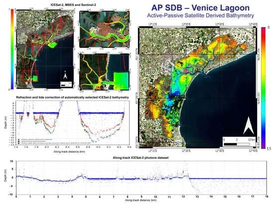
The best regression method from each depth range and seabed class was applied to the pre-processed S-2 image. The derived bathymetries were then properly merged (Figure 15).
In Figure 16, the distribution of the deviation from the derived bathymetry and the ICESat-2 points for the Gulf of Congianus is shown, along with the zoomed-in areas.

4.2. Venice Lagoon

The Venice Lagoon and the outside open sea areas were studied separately. This distinction was necessary because the two environments have very different characteristics, such as turbidity from the water and meteorological–marine phenomena, which determine their internal equilibria. The inner lagoon was studied in the range of 0–3.5 m, while the outer lagoon was studied in the range of 0–10 m.

4.2.1. ICESat-2 Bathymetry

For this area, we downloaded all the available data from the launch of ICESat-2 until the end of 2021, to have full coverage of an area with very inhomogeneous physical parameters and phase differences for the tides. Figure 17 shows the ATL03_20200101053635_00840606_005_01_gt3l beam and highlights the differences between the outer sea, on the right, and the lagoon, ranging from 5 to 12 km along a track. On the left part of the plot, we can see the hinterland of Venice, partly below the current sea level.
Figure 18a, zooming in on Section A of Figure 17, shows that for the shallow-water area of the lagoon, the extraction with the automatic algorithm was unsuccessful, mainly due to the short distance between the sea surface and the bottom. It was necessary to manually process all the ICESat-2 data in order to correctly identify the bathymetry points, and then to apply the refraction and tidal correction algorithms (Figure 18b), taking into account the different tidal phases and the different refraction coefficients of the seawater in the lagoon, according to the subdivision of Figure 17.
The automatic procedure worked well in the outer sea area, where the bathymetry was up to 10 m in a few hundred meters, making it easier to identify the seabed. Figure 19, zooming in on Section B of Figure 17, shows the automatically detected photons and the resulting depth after refraction and tidal corrections, for a portion of the ATL03_20200101053635_00840606_005_01_gt3l beam outside the lagoon, using the relevant tidal level and the refraction coefficient calculated for the specific area.

4.2.2. S-2 Seabed Classification

The Venice Lagoon is about 49 km long and up to 13 km wide, with an average depth of about 3 m, and the seabed of the lagoon consists of silt and clay mixed with sand. The study area related to the open sea outside the lagoon has a depth range of 0–20 with a sandy bottom. The Venice seabed classification was applied to the pre-processed S-2 image, defining an a priori training area in terms of sand and vegetation. The boat noise was removed during the pre-processing phase using the land mask filter.
Figure 20 highlights that almost all the seabed in the open sea is composed of sand (in yellow), while, inside the lagoon, marine vegetation (in green) is also present. The SDB was performed in the sandy areas, excluding the area with marine vegetation.

4.2.3. Regression Analysis

ICESat-2 points and the pre-processed S-2 imagery were used to train the band ratio model of Equation (4). The gross errors were discarded according to the 3-sigma criterion, and then the m0 and m1 parameters of Stumpf’s formula were calculated after a priori regression analysis to identify the best band ratio to use for each depth range.
Figure 21 shows the relationships between the two band ratios, Blue/Red and Blue/Green, and the ICESat-2 depths. The correlations were analyzed for the inner area of the lagoon in the range 0–3.5 m (Figure 21a) and for two depth ranges, 0–5 m (Figure 21b) and 5–10 m (Figure 21c), in the outside areas. The R2 values of each regression are given in the legend of each plot.
Figure 21a shows that, inside the lagoon, the correlations are noisy and not too strong. In particular, the Blue/Red ratio has a correlation coefficient R2 = 0.58, compared to the worst R2 = 0.08 for the Blue/Green ratio. Outside the lagoon, the Blue/Red correlation is stronger in the range of 0–5 m, with R2 = 0.86, against 0.60 for Blue/Green (Figure 21b). On the contrary, in the 5–10 m range, the Blue/Green correlates better (R2 = 0.56), compared to the almost null Blue/Red correlation, which is noisy and flat (Figure 21c).

4.2.4. SDB Validation and Error Analysis

The empirical Stumpf model was applied to the pre-processed S-2 image and 60% of the detected ICESat-2 points were used as “grand truth” to validate the SDB. Note that there are more ICESat-2 points in the lagoon than in the open sea (i.e., 12,615 points in the lagoon, compared to 776 and 654 points in the open sea for the 0–5 m and 5–10 m ranges, respectively) (Table 4).
Figure 22 shows three error scatter plots at different depths: 0–3.5 m inside the lagoon (Figure 22a), 0–5 m (Figure 22b), and 5–10 m (Figure 22c) outside the lagoon. Due to space limitations, we have represented the three plots related to the best calibration results obtained (i.e., with the highest R2) for each area. The band ratio Blue/Red was used for both the lagoon and the outer open sea in the 0–5 m range, while the ratio Blue/Green was used in the open sea in the 5–10 m range. The graphs show the relationship between the depth of the ICESat-2 bathymetric points (horizontal axis) and the estimated depth (SDB) (vertical axis). The red lines correspond to the 1:1 relationship, while the black line represents the regression line. The legend in the upper left gives the statistical values and the number N of the ICESat-2 points. In all figures, the scattered points are mainly distributed close to the bisector.
Table 4 complements Figure 22 by showing the statistical errors in different areas and depth ranges, and for both band ratios.
The statistics confirm that the SDB is well estimated by the Blue/Red in the very shallow water inside the lagoon, with a low RMSE and MAE of 0.63 and 0.38, respectively. Outside the lagoon, the RMSE and MAE errors increase with the increasing water depth: RMSE 0.48 and MAE 0.37 in 0–5 m, and RMSE 1.25 and MAE 0.99 in 5–10 m. The Blue/Green ratio behaves more than twice as poorly as the Blue/Red ratio in very shallow water. Instead, the Blue/Red ratio is characterized by an RMSE more than four times as high as the Blue/Green ratio in the 5–10 m range. The BIAS AVG is always close to zero, indicating that the model represents the data well. For this reason, the BIAS STD values are very close to the RMSE values.

4.2.5. SDB and BIAS Map

The best regression method from each depth range was applied to the pre-processed S-2 image.
The very-shallow-water bathymetry maps inside the lagoon were derived directly (Figure 23). Note that the SDB model certainly underestimates the depth of the navigable channels inside the lagoon, as there are no calibration points in this depth range inside the lagoon. However, the regression model is able to reproduce the bathymetric pattern also in these areas.
Outside the lagoon, the bathymetric map is given by the union of the resulting SDBs calculated using the two different regression models, for the 0–5 m and 5–10 m ranges. Each SDB model was applied to the whole area and then restricted to the respective range. However, merging the two derived bathymetric maps resulted in gaps and overlaps.
The bathymetry derived from the 0–5 m regression was used to fill in the gaps in the very-shallow-water area, by extending its validity range to 6 m, as it was characterized by lower statistical parameters than the 5–10 m regression (RMSE equal to 0.48 and 1.25 m, respectively). The 5–10 m regression was used to fill in the gaps in the deeper area.
In the case of overlapping values in the bathymetry derived from the 0–5 m and 5–10 m regressions, the difference between these values was calculated in each overlapping pixel. If the difference was small (less than the highest RMSE in absolute value, i.e., between +2 m and −2 m), the most accurate bathymetry derived from the 0–5 m regression was associated with that pixel; this was observed near the coast. On the other hand, the difference was high in deeper areas, where the 0–5 m regression greatly underestimated the depth; the difference was large and the bathymetry derived from the 5–10 m regression was associated with these pixels. Combining the map derived in this way with the 0–6 m and 5–10 m maps gave the continuous SDB shown in Figure 23.
Figure 24 shows the distribution of the BIAS from the derived bathymetry and the ICESat-2 points for areas inside and outside the Venice Lagoon. Complementing the statistics in Table 4, it can be seen that, inside the lagoon, the BIAS values are almost in the range [−0.5; 0.5], while, outside the lagoon, these values tend to increase up to 5 m depth.

5. Discussion

5.1. Comparing ICESat-2 and MBES Points in the Two AOOs

Decades of experience related to MBES measurements that guarantee the achievement of high-precision results have made it the most popular strategy in carrying out official procedures. As a result of the large market now established technologically, MBES systems can meet a wide range of requirements, even for large depths. However, the in situ approach suffers from some limitations when the operational area is characterized by shallow water, or in a coastal area where hydrographic vessels or boats are not allowed to approach. In these situations, in particular, ICESat-2 data with careful pre-processing can provide a viable alternative to MBES data.
While attesting to the “great potential for bathymetric mapping with ICESat-2”, Parrish et al. [8] recommend continuing to evaluate the accuracy of such mapping by empirically evaluating it “in additional geographic locations, using temporally coincident multibeam echosounder (MBES) data”. For this purpose, we consider the Gulf of Congianus, Sardinia (Figure 25). Due to the high gradient with which the seabed slopes, the projection of ICESat-2 data on the map results in a series of short segments, since the photons succeed in effectively reaching only the shallowest depths. However, such a seabed morphology allows hydrographic vessels or boats to move closer to the coast by reducing the area not covered by measurement. In addition, the lateral direction of the MBES sensors’ emission lobes on a steep coastline allows them to collect information related to shallower depths while still remaining in the safety zone. For this reason, in Figure 25, it can be noticed that the ICESat-2 segments used fall largely within the MBES surface.
With this overlay, it was possible to study point by point the difference between the two bathymetric measurements employed, i.e., between values associated with the same geographic coordinates. In situ MBES with high density was resampled at 10 m grid spacing, allowing the association of only a single depth value with each pixel of the image, so as to avoid having different depths associated with the same color. Subtracting then the depth values measured by ICESat-2 from those of MBES yielded the results collected in Figure 26.
With a sample of 300 points, the mean, median, and standard deviation of the MBES—ICESat-2 differences are −0.07 m, −0.09 m, and 0.40 m, respectively. The negative mean and median imply that the values measured by ICESat-2 through the ATLAS sensor are greater than those measured with MBES. In this case, the ICESat-2 data overestimate the depth, providing information about an average seafloor that is deeper than it is in reality, and, generally, a vessel relying solely on data extracted from ICESat-2 would risk entering shallower waters than expected. However, for this AOO, the study shows an average difference of about 7 cm, which is satisfying since SDB relies on multispectral images, which often, as in our study, introduce higher-dimensional approximations.
In the Venice case study, however, we find a different situation, characterized by very long ICESat-2 line projections intersecting a non-uniformly distributed MBES survey (Figure 27). As previously mentioned, the Venice Lagoon is characterized by shallow water crossed by narrow navigable channels that create an intricate system of arteries on the map. Due to the shallow depth of the lagoon bottom, the ICESat-2 lines can continuously trace the course of the lagoon from shore to shore, providing a large amount of data to the user. However, a point-by-point comparison of the difference between MBES and ICESat-2 data was not possible because only a few points are associated with the same geographic coordinates.

5.2. Comparing SDB with MBES in the Two AOOs

The availability of MBES data in both areas allows a comparison between the computed SDB bathymetry and traditional acoustics data, to check whether the results of this technology can integrate or substitute the hydrographic surveys conducted by vessels, small boats, or airborne LiDAR, having in mind the minimum requirements of the appropriate order of the International Hydrographic Organization S-44 Publication [7], listed in the Appendix in Table A1. The bar charts in Figure 28 depict the differences between the depth values measured with MBES surveys and those with the computed SDBs.
In the Gulf of Congianus, merging the results of the SDB algorithm in the two depth ranges of 0–5 m and 5–10 m, it is clear that the overall accuracy of the SDB is heavily affected by the seabed’s nature. For the rocky area in Figure 28b, the error is small up to 5 m, and then it increases rapidly accordingly to the results of the regression analysis and validation in Section 4.1, probably due to the roughness of the surface and the limited amount of good-quality points available in this range of depth after applying the automatic cleaning procedure. In contrast, in the sandy area in Figure 28a, the difference between the SBD surface and the bathymetric data is small in the whole range of 0–10 m, with a maximum error of around 5 m, which is the interface between the area of applicability of the Blue/Red and Blue/Green, where the final result is likely to be more affected by errors. In both the rocky and sandy parts of the survey, the vertical error is mainly positive, representing that the SDB algorithm in the Gulf of Congianus tends to underestimate the total depth, and the IHO requirements on the vertical uncertainty for Order 1 are always satisfied in the range of 0–5 m. For these reasons, data from the sand dataset have been used up to 10 m and from the rock dataset up to 5 m, merging them to create the final bathymetric surface. Figure 29 shows examples of the results of two different coastal shapes.
For Venice, the plot of the average errors in the lagoon area Figure 28c shows an acceptable error in the 0–3.5 m range and, for deeper bathymetry, there is a linear increase in the error with the depth, clearly showing that 3.5 m is the optical limit for the selected S-2 image in this area and period. This behavior is confirmed also by the comparison of the SDB in Figure 23 and the soundings in Figure 27: in the first one, the bathymetry computed for the channels never reaches below 5 m, while we know from the second one that there are channels that are 15 m deep and above. For the open sea area, Figure 28d shows a predominantly negative average error that reaches its maximum value of about 1.5 m around the depth of 6 m. This could be related to the high variability over time in the bathymetry of this area, taking into account that the soundings used for the accuracy check are located in the three inlets of the lagoon, characterized by strong tidal currents and frequent dredging activities that modify the bathymetry. A future study using S-2 and ICESat-2 satellite data closer in time to an investigation with acoustic techniques could provide further information on the effective capabilities of the system in areas with these characteristics. For these reasons, the datasets from the lagoon and the open sea have been separated. Since data from the open sea do not match well with the acoustic ground truth and need more studies, only the lagoon area has been considered for the resulting raster surface. Figure 30 shows the resulting surface using only depths in the range of acceptable vertical accuracy. Figure 31 highlights the four main areas of the Venice Lagoon with more detail.

5.3. SDB Method Analysis and Limitations

Our study revealed some advantages and application limitations of the SDB method integrated with ICESat-2 bathymetric data.
Regarding data collection, the ease and speed of open data access are undoubtedly relevant. After registering with the platform through online access, data are generally instantly downloadable. Otherwise, older data are provided with latency from a few minutes to several days.
Regarding the pre-processing stages of the datasets, there are operative differences between the processing of S-2 multispectral images and that of ICESat-2 data. While, for the S-2 images, there is an official and open software program released by the European Space Agency (ESA), at the time of writing this article, there is no such software for NASA data. This shortcoming has resulted in more effort in terms of time and human resources to develop ad hoc scripts.
The selection of usable beams for ICESat-2 revealed a significant problem, namely that the released data are not filtered according to their usability. In other words, being able to select only the period of interest and the geographic area of study, all data responsive to these two parameters are downloaded, but not the climatic weather conditions of the instant at which the data were collected. For this reason, for example, if the satellite had flown over the area of interest on a very cloudy day, the result of point plotting would not report any data related to either the landmass or the waterline and seabed; only a band of points in the upper part of the image would be visible, since the photons emitted would only report the presence of clouds. Thus, data quality control remains the responsibility of the operator.
The quality of the derived bathymetry depends on the multispectral image used. In this study, we benefited from using open data sources, granting free access to all necessary datasets. A limitation of this decision is the low spatial resolution of the S-2 images, which allows the derivation of bathymetric products of only an equivalent resolution. Moreover, the availability and quality of the optical data are strictly dependent on the cloud cover and the turbidity at the instant at which the data were acquired. For this reason, the bathymetric values and the accuracy of their SDB results can only be evaluated on a case-by-case basis, depending on the environmental conditions.

6. Conclusions

The growing interest in studying and monitoring coastal environments has led to significant developments in SDB methodologies and applications. However, the need for in situ measurements to calibrate and validate the multispectral images, specific to the empirical method adopted, is a limitation of this. In this context, using ICESat-2 to support the Copernicus-based SDB represents a great step forward in simplifying its application. This study explores the potential of this implementation by choosing two geomorphologically different areas as AOOs. Starting from a preliminary study conducted in the Gulf of Congianus area, characterized by a medium gradient and a rocky and sandy seabed with patches of Posidonia, we analyzed the method’s applicability by replicating the study in a particularly complex area: the Venice Lagoon. The Venice Lagoon is a predominantly sandy area, with high turbidity and patches of vegetation, in which the study of tidal and oceanographic parameters also requires further investigation. In addition, the study was conducted symmetrically considering the outer coastal area, which is no longer lagoonal, in order to compare the results.
The potential of SDB applications in the lagoon environment emerges particularly strongly from this study, especially given the growing need for continuous environmental monitoring [49,50,51,52]. As observed in the overlay of the MBES and ICESat-2 surveys within the lagoon, due to shallow water, the use of traditional means such as hydrographic boats is unsuitable and limited to navigable channels only. In other words, if the use of MBES proves to be suitable, for example, for navigation safety purposes and engineering developments, it may be inadequate for wide-area continuous monitoring purposes. Moreover, from a cartographic point of view, especially following major natural disasters, the SDB can support rapid environmental assessments. If, metrically speaking, the bathymetric derivation does not yet reach the reliability of traditional instruments, the morphological information of the seabed that it supplies can guide decision-making tasks. From this point of view, the application of the methodology, through the use of open data, provides a detailed proof-of-concept of a state-of-the-art methodology in a complex environment, favoring its reproducibility in other contexts, not only operational but also research and learning.
The analysis of the results obtained showed that the acquired bathymetries, in terms of vertical accuracy, conform to Order 1 of IHO publication S-44 [7], in the range 0–3.5 m, although with limitations in meeting the expected standards for navigational safety due to the low horizontal resolution of the multispectral image used. However, considering the high point cloud density obtainable from ICESat-2 data, future developments could investigate its reuse by employing higher-resolution multispectral imagery.

Supplementary Materials

The MATLAB code used to calculate bathymetry using Stumpf’s ratio method is available on GitHub at the following repository: https://github.com/IMATI-RS/SDB.

Author Contributions

Conceptualization, M.D., M.G., A.Q. and M.D.M; methodology, M.B., R.N., L.A., M.G., B.F., A.Q. and M.D.M.; software, M.B., R.N. and L.A.; investigation, M.B., R.N., L.A., M.D., M.G., B.F., A.Q. and M.D.M.; writing—original draft preparation, M.B., R.N., L.A., M.G., B.F., A.Q. and M.D.M.; writing—review and editing, M.B., R.N., L.A., M.G., B.F., A.Q. and M.D.M.; funding acquisition, M.D.M. All authors have read and agreed to the published version of the manuscript.

Funding

This research received no external funding.

Institutional Review Board Statement

Not applicable.

Informed Consent Statement

Not applicable.

Data Availability Statement

Not applicable.

Acknowledgments

The authors wish to acknowledge all of those who contributed to the paper: we thank the NASA National Snow and Ice Data Center (NSIDC) for distributing the ICESat-2 data, and the European Space Agency (ESA) for distributing the Sentinel-2 imagery. Warm thanks to Luca Repetti from the Istituto Idrografico della Marina for providing the tidal data and tidal elaboration.

Conflicts of Interest

The authors declare no conflict of interest.

Appendix A

Table A1. Excerpt from Table 1—Minimum Bathymetry Standards for Safety of Navigation Hydrographic Surveys [7].
CriteriaOrder 2Order 1bOrder 1aSpecial OrderExclusive Order
Depth THU [m] + [% of Depth]20 m + 10% of depth5 m + 5% of depth5 m + 5% of depth2 m1 m
Depth TVU * (a) [m] and (b)a = 1.0 m
b = 0.023
a = 0.5 m
b = 0.013
a = 0.5 m
b = 0.013
a = 0.25 m
b = 0.0075
a = 0.15 m
b = 0.0075
Feature Detection [m] or [% of Depth]Not SpecifiedNot SpecifiedCubic features >2 m, in depths down to 40 m; 10% of depth beyond 40 mCubic features >1 mCubic features >0.5 m
* TVU(d) = a 2 + ( b d ) 2 .

References

  1. OECD. Ocean Shipping and Shipbuilding. Available online: https://www.oecd.org/ocean/topics/ocean-shipping/ (accessed on 1 March 2023).
  2. UNCTAD. Review of Maritime Transport. 2022. Available online: https://unctad.org/topic/transport-and-trade-logistics/review-of-maritime-transport (accessed on 1 March 2023).
  3. Pascual, M. Cables and Pipelines. 16 February 2018. Available online: https://maritime-spatial-planning.ec.europa.eu/sites/default/files/sector/pdf/mspforbluegrowth_sectorfiche_cablespipelines.pdf (accessed on 27 February 2023).
  4. Díaz, H.; Guedes Soares, C. Review of the current status, technology and future trends of offshore wind farms. Ocean. Eng. 2020, 209, 107381. [Google Scholar] [CrossRef]
  5. NOAA. Introduction to Multibeam—NOAA Hydro Training 2009. Available online: https://slideplayer.com/slide/5974610/ (accessed on 28 January 2023).
  6. Khomsin, D.G.P.; Saputro, I. Comparative analysis of singlebeam and multibeam echosounder bathymetric data. IOP Conf. Mater. Sci. Eng. 2021, 1052, 012015. [Google Scholar] [CrossRef]
  7. IHO. S-44 IHO Standards for Hydrographic Surveys—Ed. 6. 2020. Available online: https://iho.int/uploads/user/pubs/standards/s-44/S-44_Edition_6.0.0_EN.pdf (accessed on 28 February 2023).
  8. Parrish, C.E.; Magruder, L.A.; Neuenschwander, A.L.; Forfinski-Sarkozi, N.; Alonzo, M.; Jasinski, M. Validation of ICESat-2 ATLAS Bathymetry and Analysis of ATLAS’s Bathymetric Mapping Performance. Remote Sens. 2019, 11, 1634. [Google Scholar] [CrossRef] [Green Version]
  9. Zhang, X.; Chen, Y.; Le, Y.; Zhang, D.; Yan, Q.; Dong, Y.; Han, W.; Wang, L. Nearshore Bathymetry Based on ICESat-2 and Multispectral Images: Comparison between Sentinel-2, Landsat-8, and Testing Gaofen-2. IEEE J. Sel. Top. Appl. Earth Obs. Remote Sens. 2022, 15, 2449–2462. [Google Scholar] [CrossRef]
  10. Cahalane, C.; Magee, A.; Monteys, X.; Casal, G.; Hanafin, J.; Harris, P. A comparison of Landsat 8, RapidEye and Pleiades products for improving empirical predictions of satellite-derived bathymetry. Remote Sens. Environ. 2019, 233, 111414. [Google Scholar] [CrossRef]
  11. Poursanidis, D.; Traganos, D.; Reinartz, P.; Chrysoulakis, N. On the use of Sentinel-2 for coastal habitat mapping and satellite-derived bathymetry estimation using downscaled coastal aerosol band. Int. J. Appl. Earth Obs. Geoinf. 2019, 80, 58–70. [Google Scholar] [CrossRef]
  12. Casal, G.; Monteys, X.; Hedley, J.; Harris, P.; Cahalane, C.; McCarthy, T. Assessment of empirical algorithms for bathymetry extraction using Sentinel-2 data. Int. J. Remote Sens. 2019, 40, 2855–2879. [Google Scholar] [CrossRef]
  13. Casal, G.; Harris, P.; Monteys, X.; Hedley, J.; Cahalane, C.; McCarthy, T. Understanding satellite-derived bathymetry using Sentinel 2 imagery and spatial prediction models. GISci. Remote Sens. 2020, 57, 271–286. [Google Scholar] [CrossRef]
  14. Hochberg, E.; Andrefouet, S.; Tyler, M. Sea surface correction of high spatial resolution Ikonos images to improve bottom mapping in near-shore environments. IEEE Trans. Geosci. Remote Sens. 2003, 41, 1724–1729. [Google Scholar] [CrossRef]
  15. Ohlendorf, S.; Müller, A.; Heege, T.; Cerdeira-Estrada, S.; Kobryn, H.T. Bathymetry mapping and sea floor classification using multispectral satellite data and standardized physics based data processing. In Proceedings of the Remote Sensing of the Ocean, Sea Ice, Coastal Waters, and Large Water Regions 2011, Prague, Czech Republic, 21–22 September 2011; Volume 8175, pp. 33–41. [Google Scholar]
  16. Lubac, B.; Burvingt, O.; Nicolae Lerma, A.; Sénéchal, N. Performance and Uncertainty of Satellite-Derived Bathymetry Empirical Approaches in an Energetic Coastal Environment. Remote Sens. 2022, 14, 2350. [Google Scholar] [CrossRef]
  17. Caballero, I.; Stumpf, R.P. Retrieval of nearshore bathymetry from Sentinel-2A and 2B satellites in South Florida coastal waters. Estuar. Coast. Shelf Sci. 2019, 226, 106277. [Google Scholar] [CrossRef]
  18. Brando, V.E.; Anstee, J.M.; Wettle, M.; Dekker, A.G.; Phinn, S.R.; Roelfsema, C. A physics based retrieval and quality assessment of bathymetry from suboptimal hyperspectral data. Remote Sens. Environ. 2009, 113, 755–770. [Google Scholar] [CrossRef]
  19. Stumpf, R.P.; Holderied, K.; Sinclair, M. Determination of water depth with high-resolution satellite imagery over variable bottom types. Limnol. Oceanogr. 2003, 48, 547–556. [Google Scholar] [CrossRef]
  20. Lyzenga, D.; Malinas, N.; Tanis, F. Multispectral bathymetry using a simple physically based algorithm. IEEE Trans. Geosci. Remote Sens. 2006, 44, 2251–2259. [Google Scholar] [CrossRef]
  21. Xie, C.; Chen, P.; Pan, D.; Zhong, C.; Zhang, Z. Improved Filtering of ICESat-2 Lidar Data for Nearshore Bathymetry Estimation Using Sentinel-2 Imagery. Remote Sens. 2021, 13, 4303. [Google Scholar] [CrossRef]
  22. Apicella, L.; De Martino, M.; Ferrando, I.; Quarati, A.; Federici, B. Deriving Coastal Shallow Bathymetry from Sentinel 2-, Aircraft- and UAV-Derived Orthophotos: A Case Study in Ligurian Marinas. J. Mar. Sci. Eng. 2023, 11, 671. [Google Scholar] [CrossRef]
  23. Apicella, L.; De Martino, M.; Quarati, A. Copernicus User Uptake: From Data to Applications. ISPRS Int. J. Geo-Inf. 2022, 11, 121. [Google Scholar] [CrossRef]
  24. European Comission. General Presentations of the Copernicus Programme—What is the Copernicus Programme? 2016. Available online: https://www.youtube.com/playlist?list=PLNxdHvTE74JztZhhmA5A5GylDcIKPT0fD (accessed on 30 May 2023).
  25. ESA. Mission Objectives. Available online: https://sentinel.esa.int/web/sentinel/missions/sentinel-2/mission-objectives (accessed on 8 January 2023).
  26. Drusch, M.; Gascon, F. GMES Sentinel-2 Mission Requirement Document; ESA: Paris, France, 2010. [Google Scholar]
  27. ESA. Sentinel-2. Available online: https://sentinel.esa.int/web/sentinel/missions/sentinel-2 (accessed on 8 January 2023).
  28. Forfinski-Sarkozi, N.A.; Parrish, C. Analysis of MABEL Bathymetry in Keweenaw Bay and Implications for ICESat-2 ATLAS. Remote Sens. 2016, 8, 772. [Google Scholar] [CrossRef] [Green Version]
  29. Jasinski, M.F.; Stoll, J.D.; Cook, W.B.; Ondrusek, M.; Stengel, E.; Brunt, K. Inland and Near-Shore Water Profiles Derived from the High-Altitude Multiple Altimeter Beam Experimental Lidar (MABEL). J. Coast. Res. 2016, 76, 44–55. [Google Scholar] [CrossRef]
  30. Ma, Y.; Xu, N.; Liu, Z.; Yang, B.; Yang, F.; Wang, X.H.; Li, S. Satellite-derived bathymetry using the ICESat-2 lidar and Sentinel-2 imagery datasets. Remote Sens. Environ. 2020, 250, 112047. [Google Scholar] [CrossRef]
  31. Thomas, N.; Pertiwi, A.P.; Traganos, D.; Lagomasino, D.; Poursanidis, D.; Moreno, S.; Fatoyinbo, L. Space-borne cloud-native satellite-derived Bathymetry (SDB) models using ICESat-2 and sentinel-2. Geophys. Res. Lett. 2021, 48, e2020GL092170. [Google Scholar] [CrossRef]
  32. Albright, A.; Glennie, C. Nearshore bathymetry from fusion of Sentinel-2 and ICESat-2 observations. IEEE Geosci. Remote Sens. Lett. 2020, 18, 900–904. [Google Scholar] [CrossRef]
  33. Babbel, B.J.; Parrish, C.E.; Magruder, L.A. ICESat-2 elevation retrievals in support of satellite-derived bathymetry for global science applications. Geophys. Res. Lett. 2021, 48, e2020GL090629. [Google Scholar] [CrossRef]
  34. Ranndal, H.; Sigaard Christiansen, P.; Kliving, P.; Baltazar Andersen, O.; Nielsen, K. Evaluation of a Statistical Approach for Extracting Shallow Water Bathymetry Signals from ICESat-2 ATL03 Photon Data. Remote Sens. 2021, 13, 3548. [Google Scholar] [CrossRef]
  35. Niroumand-Jadidi, M.; Bovolo, F.; Bruzzone, L.; Gege, P. Physics-based Bathymetry and Water Quality Retrieval Using PlanetScope Imagery: Impacts of 2020 COVID-19 Lockdown and 2019 Extreme Flood in the Venice Lagoon. Remote Sens. 2020, 12, 2381. [Google Scholar] [CrossRef]
  36. Gianinetto, M.; Lechi, G. A DNA algorithm for the batimetric mapping in the lagoon of Venice using QuickBird multispectral data. In Proceedings of the 20th ISPRS Congress, Geo-Imagery Bridging Continents Volume: The International Archive of the Photogrammetry, Remote Sensing and Spatial Information Sciences, Istanbul, Turkey, 12–23 July 2004; pp. 94–99. [Google Scholar]
  37. EO-Portal. ICESat-2. Available online: https://www.eoportal.org/satellite-missions/icesat-2 (accessed on 7 February 2023).
  38. NASA. ICESat-2, How it Works. Available online: https://icesat-2.gsfc.nasa.gov/how-it-works (accessed on 7 February 2023).
  39. NASA. ICESat-2, Technical Specs. Available online: https://icesat-2.gsfc.nasa.gov/science/specs (accessed on 7 February 2023).
  40. Neumann, A.; Brenner, D.H. ATLAS/ICESat-2 L2A Global Geolocated Photon Data, Version 2; NSIDC: Boulder, CO, USA, 2018. [Google Scholar] [CrossRef]
  41. Magruder, L.A.; Brunt, K.M. Performance Analysis of Airborne Photon- Counting Lidar Data in Preparation for the ICESat-2 Mission. IEEE Trans. Geosci. Remote Sens. 2018, 56, 2911–2918. [Google Scholar] [CrossRef]
  42. NSIDC. Open Access NASA Data for Your Research and Studies. 2022. Available online: https://nsidc.org/data/data-programs/nsidc-daac (accessed on 7 February 2023).
  43. The icepyx Developers. icepyx: Python Tools for Obtaining and Working with ICESat-2 data. 2023. Available online: https://github.com/icesat2py/icepyx (accessed on 30 May 2023).
  44. Austin, R.W.; Halikas, G. The Index of Refraction of Seawater; Scripps Institution of Oceanography: San Diego, CA, USA, 1976. [Google Scholar]
  45. Sentinel Application Platform (SNAP). ESA. Brockmann Consult, Skywatch, Sensar and C-S. Available online: https://step.esa.int/main/toolboxes/snap (accessed on 30 May 2023).
  46. QGIS Development Team. QGIS Geographic Information System. Open Source Geospatial Foundation. 2022. Available online: http://qgis.osgeo.org (accessed on 30 May 2023).
  47. GRASS Development Team. Geographic Resources Analysis Support System (GRASS) Software, Version 8.2. Open Source Geospatial Foundation. 2022. Available online: https://grass.osgeo.org (accessed on 30 May 2023).
  48. RUS Service. Nearshore Bathymetry Derivation with Sentinel-2. 2021. Available online: https://eo4society.esa.int/wp-content/uploads/2022/01/COAS01_BathymetryDerivation_Greece.pdf (accessed on 27 February 2023).
  49. Ivajnšič, D.; Kaligarič, M.; Fantinato, E.; Del Vecchio, S.; Buffa, G. The fate of coastal habitats in the Venice Lagoon from the sea level rise perspective. Appl. Geogr. 2018, 98, 34–42. [Google Scholar] [CrossRef] [Green Version]
  50. D’Alpaos, A.; Finotello, A.; Tognin, D.; Carniello, L.; Marani, M. The Venice Lagoon foreshadows the fate of coastal systems under climate change and increasing human pressure. In Proceedings of the GU General Assembly 2023, Vienna, Austria, 24–28 April 2023. EGU23-10125. [Google Scholar] [CrossRef]
  51. Regione del Veneto. Emergenza Crisi Idrica. 2022. Available online: https://www.regione.veneto.it/web/gestioni-commissariali-e-post-emergenze/crisiidrica2022/ (accessed on 3 March 2023).
  52. World Economic Forum. Italy Faces New Drought Alert as Venice Canals Run Dry. 2023. Available online: https://www.weforum.org/agenda/2023/02/heres-how-italys-dry-canals-in-venice-spell-trouble-for-this-year (accessed on 3 March 2023).
Figure 1. Representation of the two areas of operation (AOOs): (a) Gulf of Congianus, (b) Venice Lagoon and the open sea outside it. (Picture generated using Google Earth, 5 February 2023).
Remotesensing 15 02944 g001
Figure 2. Representation of S-2 images selected and cropped according to areas of interest: (a) Gulf of Congianus and (b) Venice Lagoon.
Remotesensing 15 02944 g002
Figure 3. Projection of soundings contained in the trajectories of ICESat-2 beams selected and cleaned for the study areas: (a) Gulf of Congianus and (b) Venice Lagoon.
Remotesensing 15 02944 g003
Figure 4. MBES bathymetric surveys of (a) Venice Lagoon and (b) Gulf of Congianus. To the left of each image is the graduated scale reflecting the reference depth.
Remotesensing 15 02944 g004
Figure 5. (a) Geographical distribution of tide gauges inside the Venice Lagoon and (b) the geographical division in two macro areas inside and outside the lagoon, with further subdivisions inside them.
Remotesensing 15 02944 g005
Figure 6. Example of a profile obtained from the first phase of ICESat-2 data processing, with the photons dataset referenced to ellipsoid WGS84 (blue) and the photons shifted and referenced to the geoid EGM-2008 (green).
Remotesensing 15 02944 g006
Figure 7. The measured height (blue dots) relative to the geoid was transformed into the water column depth (fuchsia dots) relative to a zero level (yellow line), which represents the shift of the water surface (red line) as a reference level. Zoom-in on the 16–17 m along-track distance of the profile in Figure 6.
Remotesensing 15 02944 g007
Figure 8. Bathymetry points (in purple) corrected by refraction (green dots) and their tide level correction (red dots) relative to a specific date and time, using local tide gauge measurements. The ICESat-2 data were acquired during a lower tide than the reference time, causing an upward shift.
Remotesensing 15 02944 g008
Figure 9. Example of tide correction applied to the ICESat-2 and MBES data to reference them to the time of S-2 image acquisition.
Remotesensing 15 02944 g009
Figure 10. The profile obtained from the ATL03_20200114165545_02900602_005_01_gt2r beam at the end of the Data automatic download and preparation phase and after referencing to the geoid EGM-2008. The diagram shows the profile of the emerged land, the waterline, and the seabed, which remains well distinct from the noise points, especially in the more superficial layers. The profile section in rectangle A is zoomed in Figure 11.
Remotesensing 15 02944 g010
Figure 11. The bathymetric points (green dots) extracted automatically, and their resulting depths after the refraction and tide level correction (red dots) relative to a specific date and time, using local tide gauge measurement and local temperature and salinity data (Section A from Figure 10).
Remotesensing 15 02944 g011
Figure 12. Result of the seabed classification process in the Gulf of Congianus. Seabed classes are sand (yellow), rock (grey), and vegetation and other seabed cover (green).
Remotesensing 15 02944 g012
Figure 13. Calibration results, showing the relationship between the Blue/Green ratio (in green) or the Blue/Red ratio (in red) and the depth of the ICESat-2 calibration point set. (a) Sand, 0–5 m; (b) Rocks, 0–5 m; (c) Sand, 5–10 m; (d) Rocks, 5–10 m. Gulf of Congianus.
Remotesensing 15 02944 g013aRemotesensing 15 02944 g013b
Figure 14. SDB validation: error scatter plots in different depth ranges, showing the relationship between the depth of the ICESat-2 bathymetric points and the estimated SDB. N is the number of ICESat-2 points used. (a) Sand, 0–5 m; (b) Rocks, 0–5 m; (c) Sand, 5–10 m; (d) Rocks, 5–10 m. Gulf of Congianus.
Remotesensing 15 02944 g014
Figure 15. SDBs obtained down to 5 m depth using the Blue/Red ratio for sand and rocks and using Blue/Green ratio in the 5–10 m range for sand. No bathymetries were derived for rocky areas in the 5–10 m range.
Remotesensing 15 02944 g015
Figure 16. BIAS distribution for the Gulf of Congianus.
Remotesensing 15 02944 g016
Figure 17. Profile obtained from beam ATL03_20200101053635_00840606_005_01_gt3l at the end of phase 1 Data automatic download and preparation, with a sub-section, and after the referencing to the geoid EGM-2008. The main elements of this image are the profile of the hinterland of Venice partially below the current sea level on the left, the Venice Lagoon in the middle, and the open sea with the seabed on the right. The lagoon shows a complex structure of water layers. The profile sections in rectangles A and B are zoomed in Figure 18 and Figure 19.
Remotesensing 15 02944 g017
Figure 18. (a) Automatically extracted bathymetric points (red dots). The highlighted points (red dots) are not representative of the seabed. (b) Manually extracted bathymetric points (green dots) and their resulting depths after refraction and tidal level correction (red dots) relative to a specific date and time, using local tide gauge measurements and local temperature and salinity data. Section A of Figure 17 relating to the lagoon area.
Remotesensing 15 02944 g018aRemotesensing 15 02944 g018b
Figure 19. Automatically extracted bathymetric points (green dots) and their resulting depths after refraction and tide level correction (red dots) relative to a specific date and time, using local tide gauge measurements and local temperature and salinity data. Section B from the outer sea in Figure 17.
Remotesensing 15 02944 g019
Figure 20. Result of the seabed classification process in the Venice Lagoon. Classes of the seabed are identified as sand in yellow areas and marine vegetation in green.
Remotesensing 15 02944 g020
Figure 21. Results of the calibration phase showing the relationship between the Blue/Green ratio (green color) or the Blue/Red ratio (red color) and the depth of the ICESat-2 calibration point sets. (a) Lagoon; (b) Open sea, 0–5 m; (c) Open sea, 5–10 m. Venice Lagoon.
Remotesensing 15 02944 g021
Figure 22. SDB validation: error scatter plots of the relationship between the depth of the ICESat-2 bathymetric points and the estimated depth (SDB). The black line is the regression line. (a) Lagoon; (b) Open sea, 0–5 m; (c) Open sea, 5–10 m. Venice Lagoon.
Remotesensing 15 02944 g022
Figure 23. Sentinel-derived bathymetry (SDB) for the Venice Lagoon and the open sea area in front of Venice.
Remotesensing 15 02944 g023
Figure 24. BIAS distribution for the areas inside and outside the Venice Lagoon.
Remotesensing 15 02944 g024
Figure 25. Overlapping of ICESat-2 bathymetric points (yellow points) and MBES bathymetric data (the colored area from the range red–blue) and zoom-in of the coastal area with more ICESat-2 points. Sardinia.
Remotesensing 15 02944 g025
Figure 26. Histogram of the differences in the depth values measured by ICESat-2 and MBES in the Gulf of Congianus.
Remotesensing 15 02944 g026
Figure 27. ICESat-2 (red points) and MBES (area colored from red to blue) data. Zoom-in of two characteristic areas. Venice Lagoon.
Remotesensing 15 02944 g027
Figure 28. Bar charts of the differences in the depth values measured with MBES surveys The red dashed line represents the ±0.5 m range, the Total Vertical Uncertainty for the Order 1 Standard of the IHO-S44 Publication. (a) MBES-SDB, Gulf of Congianus, Sand; (b) MBES-SDB, Gulf of Congianus, Rocks; (c) MBES-SDB, Venice, Lagoon; (d) MBES-SDB, Venice, Sea.
Remotesensing 15 02944 g028
Figure 29. SDB results in the Gulf of Congianus area after a 5 m depth (filter only to rocky seabed areas) is applied for the range of acceptability of vertical uncertainty of IHO standards. On the left are the S-2 images and on the right are the SDB results. (a) Cugnana Gulf, the shallower part of the case study area; (b) a jagged coastal area from the Marinella and Aranci Gulfs.
Remotesensing 15 02944 g029
Figure 30. SDB results from the Venice Lagoon area, after a 3.5 m depth is filter applied for the range of acceptability of vertical uncertainty of IHO standards.
Remotesensing 15 02944 g030
Figure 31. SDB results from the Venice Lagoon area, after a 3.5 m depth filter is applied for the range of acceptability of vertical uncertainty of IHO standards. On the left are the S-2 images, and on the right are the SDB results: (a) the northern part of the Venice Lagoon, (b) the lagoon area near Venice Town, (c) the lagoon area near Malamocco, (d) the lagoon area near Chioggia Town.
Remotesensing 15 02944 g031
Table 1. Detailed information of the study areas, the ICESat-2 and S-2 rev products, and the in situ survey datasets. Gulf of Congianus, Sardinia.
SiteGulf of Congianus, Sardinia
Latitude40°58.8′N–41°8.4′N
Longitude009°30.6′E–009°40.2′E
ICESat-2
Track-beams
(Tot.: 7)
ATL03_20200114165545_02900602_005_01—gt2r
ATL03_20200114165545_02900602_005_01—gt3r
ATL03_20200613215507_12120706_005_01—gt1l
ATL03_20200613215507_12120706_005_01—gt2l
ATL03_20200613215507_12120706_005_01—gt3l
ATL03_20200912173455_12120806_005_01—gt1l
ATL03_20201111023110_07320902_005_01—gt1l
S-222 June 2020–S2B_MSIL2A
In situ dataMBES Kongsberg EM 2040C (1 September 2016–31 October 2016)
Oceanographic Data—Copernicus Marine Service
Tidal Data—Tide Gauge IIM in La Maddalena
Table 2. Detailed information of the study areas, the ICESat-2 and S-2 products, and the in situ survey datasets. Venice Lagoon.
SiteVenice Lagoon, Veneto
Latitude45°10.8′N–45°36′N
Longitude12°7.8′E–12°42′E
ICESat-2
Track-beams
(Tot.: 73)
ATL03_20181128122207_09300102_005_01All beams
ATL03_20181205002119_10290106_005_011l-3l-3r
ATL03_20190227080209_09300202_005_011r-2l-2r
ATL03_20190305200120_10290206_005_011l-2l-3l-3r
ATL03_20190730004527_04880402_005_013l-3r
ATL03_20190827232133_09300402_005_011l-2l
ATL03_20190903112043_10290406_005_011l
ATL03_20190925215739_13720402_005_011l-1r-2r
ATL03_20191225173726_13720502_005_011l
ATL03_20200101053635_00840606_005_012l-2r-3l-3r
ATL03_20200503234405_05870706_005_011l-1r
ATL03_20200601222008_10290706_005_011l-1r-2l-2r-3l
ATL03_20200630205609_00840806_005_013l-3r
ATL03_20200727072442_04880802_005_01All beams
ATL03_20201124014034_09300902_005_011l-1r-2r-3r
ATL03_20201130133944_10290906_005_011l-1r-2r-3r
ATL03_20210124224424_04881002_005_011l-3l-3r
ATL03_20210301091935_10291006_005_012l-2r-3l-3r
ATL03_20210629033531_00841206_005_013r
ATL03_20210927231529_00841306_005_01All beams
ATL03_20211024094406_04881302_005_012l-2r-3l-3r
S-219 March 2020 - S2A_MSIL2A
In situ dataSoundings from the IIM BathyDataBase (2013–2019)
Oceanographic data—ARPA (Venice) and Copernicus Marine Service
Tidal data—ISPRA (Venice)
Table 3. Statistical errors (in m): RMSE and MAE for model validation, and the standard deviation and the average value of the BIAS between the SDB and the ICESat GPs for the two band ratios and the two ranges of depth (0–5 m and 0–10 m), in sandy and rocky areas. Gulf of Congianus.
Blue/RedBlue/Green
SandRocksSandRocks
0–5 mN2514925150
RMSE0.461.130.651.79
MAE0.370.820.451.26
BIAS_AVG−0.01−0.04−0.030.04
BIAS_STD0.471.140.671.79
5–10 mN40124012
RMSE5.714.590.784.95
MAE4.893.380.614.17
BIAS_AVG1.731.900.060.23
BIAS_STD5.564.480.795.21
Table 4. Statistical values (in m) related to the model validation and the BIAS between the SDB and the ICESat GPs, for the ratios of the two bands and the different ranges: 0–3.5 m inside the lagoon, 0–5 m and 5–10 m in the open sea outside the lagoon.
Blue/RedBlue/Green
Lagoon
0–3.5 mN12,61512,615
RMSE0.632.05
MAE0.381.52
BIAS_AVG−0.04−0.05
BIAS_STD0.632.05
Open sea
0–5 mN776776
RMSE0.481.10
MAE0.370.74
BIAS_AVG−0.07−0.13
BIAS_STD0.471.09
5–10 mN654654
RMSE5.471.25
MAE4.650.99
BIAS_AVG0.310.03
BIAS_STD5.481.25
Disclaimer/Publisher’s Note: The statements, opinions and data contained in all publications are solely those of the individual author(s) and contributor(s) and not of MDPI and/or the editor(s). MDPI and/or the editor(s) disclaim responsibility for any injury to people or property resulting from any ideas, methods, instructions or products referred to in the content.

