

Radar Active Jamming Recognition under Open World Setting

1
School of Electronic and Information, Hangzhou Dianzi University, Hangzhou 310018, China
2
School of Communication Engineering, Hangzhou Dianzi University, Hangzhou 310018, China
3
School of Electrical and Computer Engineering, Royal Melbourne Institute of Technology (RMIT University), Melbourne 3000, Australia
*
Author to whom correspondence should be addressed.
Remote Sens. 2023, 15(16), 4107; https://0-doi-org.brum.beds.ac.uk/10.3390/rs15164107
Submission received: 30 June 2023
/
Revised: 17 August 2023
/
Accepted: 18 August 2023
/
Published: 21 August 2023
(This article belongs to the Special Issue Artificial Intelligence-Driven Methods for Remote Sensing Target and Object Detection)
Abstract
:To address the issue that conventional methods cannot recognize unknown patterns of radar jamming, this study adopts the idea of zero-shot learning (ZSL) and proposes an open world recognition method, RCAE-OWR, based on residual convolutional autoencoders, which can implement the classification of known and unknown patterns. In the supervised training phase, a residual convolutional autoencoder network structure is first constructed to extract the semantic information from a training set consisting solely of known jamming patterns. By incorporating center loss and reconstruction loss into the softmax loss function, a joint loss function is constructed to minimize the intra-class distance and maximize the inter-class distance in the jamming features. Moving to the unsupervised classification phase, a test set containing both known and unknown patterns is fed into the trained encoder, and a distance-based recognition method is utilized to classify the jamming signals. The results demonstrate that the proposed model not only achieves sufficient learning and representation of known jamming patterns but also effectively identifies and classifies unknown jamming signals. When the jamming-to-noise ratio (JNR) exceeds 10 dB, the recognition rate for seven known jamming patterns and two unknown jamming patterns is more than 92%.
1. Introduction
Radar faces increasingly complex electronic countermeasures, with various new types of radar jamming patterns continuously emerging as challenges [1,2]. The accurate recognition of radar jamming is a precondition and key to implementing anti-jamming measures, and automatic recognition of radar jamming patterns can effectively improve the target detection and tracking performance of radar. Therefore, jamming pattern recognition has always been a research hotspot in anti-jamming technology [3,4]. Suppression jamming by emitting high-power noise signals is not only effective for linear frequency modulated (LFM) radar systems but also for other modulated radar systems, making it the most widely used [5]. Therefore, this paper focuses on the recognition of suppression jamming. Its main patterns include amplitude modulation jamming (AMJ), frequency modulation jamming (FMJ), comb spectrum jamming (CJ), phase modulation jamming (PMJ), swept jamming (SJ), etc. Conventional jamming pattern detection and classification methods are generally based on feature engineering. Firstly, multi-dimensional features of signal in time domain, frequency domain, and transform domain are extracted, including features such as moment kurtosis, moment skewness, envelope fluctuation, noise factor [6,7,8,9], singular spectrum features [10], bispectrum features [11] and other signal features. Then, with the help of machine learning-based classifiers, such as support vector machine (SVM ) [12], decision trees [13], and back propagation (BP) neural networks [12], classifications are accomplished. However, feature engineering-based classification methods are time-consuming and require expert experience, especially when the transform domain features are large, the classification performance has limited room for improvement, and the recognition rate is low in strong noise environment.
With the development of deep learning (DL) technology, the feature extraction capability of neural networks has been improving, and classification methods based on DL are emerging. In [14], A novel hybrid framework of optimized deep learning models combined with multi-sensor fusion is developed for condition diagnosis of concrete arch beam, and the results demonstrate that the method can achieve the classification of structural damage with limited sensors and high levels of uncertainties.
Convolutional neural networks (CNNs), due to their network architecture which incorporates weight sharing and small local receptive fields, have significantly reduced the number of node connections compared to conventional neural networks. This simplification of network connections has made CNNs widely applied in deep learning models [15,16,17]. CNNs can train their parameters using jamming signals, eliminating the need for manual feature extraction and the design of decision trees for classification criteria. As a result, CNNs have been extensively used in the research of classifying and recognizing radar jamming signals [18].
In [19], a jamming recognition algorithm based on improved LeNet·CNN network was designed which extracted one-dimensional radar received signals and adjusted the network structure parameters to achieve optimal performance for the recognition of jamming signals. Ref. [20] obtained the time-frequency spectrogram of jamming signals by short-time Fourier transform, combined with the improved VGGNet·16 network model for feature learning and training, and the simulation verified that the algorithm is still effective for the identification of six kinds of mixed jamming. Ref. [21] adopted an adaptive cropping algorithm to crop most of the redundant information of the time-frequency image and kept the complete information of the jamming in the CNN for training, and finally achieved the recognition of nine kinds of jamming signals with high accuracy and fast iteration. In [22], a 1D CNN-based radar jamming signal classification model was proposed to achieve the classification of 12 typical jamming signals by putting the real and imaginary parts of jamming signals into the parallel network for training. In [23], a CNN was constructed using the real and imaginary parts of the signal as inputs. With sufficient training samples, this method demonstrated excellent recognition capabilities. The mentioned papers primarily address the issue of recognizing jamming when there are sufficient labeled samples. However, [6,24,25] considered the case of insufficient labeled samples. Ref. [6] proposed a method based on a time-frequency self-attentive mechanism. The recognition rate for most of the patterns of jamming reaches 90% when the samples with labels account for 3%. In [24], Tian et al. inputed features obtained through empirical mode decomposition and wavelet decomposition into the network. Simulations conducted on a dataset consisting of only 8400 samples showed that the recognition rates for four types of jamming were all above 90% when the JNR exceeded 6 dB. In [25], a large number of unlabeled samples were first used to train an jamming recognition network to extract valuable features. Then, a small number of labeled samples were used to improve the classification accuracy.
Although the application of deep learning technology in radar jamming recognition is rapidly developing, the current methods still suffer from the closed-set assumption, i.e., the existing methods assume that the jamming patterns are included in the training set. However, in the actual battlefield environment, the enemy may invent new jamming patterns, making it challenging to collect data for all patterns in the training set, so the actual radar jamming environment is an open set scenario, i.e., the test environment is likely to have jamming patterns that do not exist in the training jamming library. In the actual open set jamming scenario, when a jamming pattern that does not exist in the training jamming library appears in the test environment, the existing radar jamming identification methods will incorrectly identify this unknown jamming as one of the known jamming patterns. In [26], Zhou et al. first investigated the open set recognition problem for radar jamming; however, the method can only detect or reject the unknown patterns, but cannot effectively identify the unknown patterns. How to further classify these unknown pattern signals remains a challenging task, and it falls under the research domain of open world recognition (OWR).
Currently, OWR techniques have been applied in target recognition of synthetic aperture radar (SAR) images. In [27], a hierarchical embedding and incremental evolutionary network (HEIEN) was designed for when there are fewer unknown target training sets in open scenarios, which requires only a small number of unknown target samples for effective model training. A more stable feature space was built in [28], which has better interpretability. In testing, experiments on a dataset containing seven known targets and one unknown target show that the method improves the reliability of recognizing unknown targets. In [29], Song et al. used physical EM simulation images of targets at different azimuths as training data in order to learn the features of unknown targets. An accuracy of 91.93% can be achieved in a recognition task with a dataset containing nine known targets and one unknown target.
Nevertheless, OWR is just starting in radar jamming pattern recognition. Zero-shot learning (ZSL) [30,31] is an effective approach to address the challenge of open world recognition. The most typical implementation of ZSL is based on feature mapping. The goal of this approach is to learn the mapping relationship between the original signal space and the semantic feature space using the known jamming patterns. This learned relationship is then generalized to the unknown pattern dataset, enabling recognition and classification of unknown patterns using the semantic features. ZSL can be classified into two types: traditional zero-shot learning (TZSL) and generalized zero-shot learning (GZSL) [32]. TZSL assumes that the training patterns are known, while the testing patterns are unknown, and there is mutual exclusion between the training and testing patterns. GZSL assumes that the training patterns include both known and unknown patterns in the testing phase. GZSL has a more relaxed experimental setting, which better reflects real-world scenarios. Therefore, in this paper, we consider the GZSL scenario.
To address the challenge of existing methods being unable to classify unknown jamming patterns specifically, this paper adopts the idea of ZSL and conducts research on jamming patterns recognition in an open world scenario. We propose a residual convolutional autoencoder-based radar jamming open world recognition algorithm, abbreviated as RCAE-OWR.
In summary, the main contributions of this paper are as follows:
- In order to address the limitations of existing radar jamming pattern recognition methods, which are mostly closed-set recognition or simply rejecting unknown patterns, we propose a zero-shot learning approach based on residual conventional autoencoders. This method does not require prior information about the patterns of jamming and can classify both known and unknown patterns using distance-based recognition methods.
- A hybrid loss function consisting of cross-entropy loss, center loss and reconstruction loss is introduced to recognize different patterns of jamming signals. Where the cross-entropy loss makes the features obtained from the mapping network divisible, and to some extent widens the distance among different patterns, the center loss makes it easier to delineate the boundaries of the various patterns, and the reconstruction loss ensures that the most essential characterization of the pattern features is learned from the known patterns dataset.
- Through extensive experimental simulations, we evaluate the open world recognition performance of the proposed algorithm and investigate the influence of JNR and the number of unknown patterns on the algorithm’s performance. The simulation results demonstrate that the proposed algorithm achieves effective recognition of both known and unknown patterns, especially in high-JNR environments.
2. Jamming Signal Modeling
In radar jamming and anti-jamming training, the signals received by the radar receiver include radar echo signals, jamming signals and noise signals, which can be expressed as follows:
where denotes the total signal received by the radar, represents the echo signal, means the jamming signal, and is the noise signal.
2.1. Echo Signal
Typical modulation types of radar echo signals include continuous wave (CW), linear frequency modulation (LFM), phase shift keying (PSK), frequency shift keying (FSK), etc. LFM, with its frequency linearly changing over time, is the most widely used. Therefore, in this paper, we focus on studying the typical echo signal of LFM, which can be expressed as follows [33]:
where i denotes the pulse sequence; rect represents the i-th rectangular pulse with a width of is the pulse repetition period; is the pulse width; is the radar center frequency; B means the bandwidth; and is the LFM coefficient.
2.2. Jamming Signal
In this paper, we select nine typical radar active jamming patterns as the research objects, including: radio noise jamming (RNJ) [26], amplitude modulation jamming (AMJ) [34], frequency modulation jamming (FMJ) [34], comb spectrum jamming (CJ) [13], phase modulation jamming (PMJ) [34], linear sweep frequency jamming (LSFJ) [34], non-linear sweep frequency jamming (NLSFJ) [35], hopping frequency jamming (HFJ) [35] and periodic Gaussian pulse jamming (PGJ) [36].
2.2.1. Radio Noise Jamming
RNJ is a narrowband Gaussian process generated by filtering and then amplifying the noise signal. Its mathematical model is expressed as:
where obeys a Gaussian distribution, is the carrier frequency, and is the initial phase, following a uniform distribution on .
2.2.2. Amplitude Modulation Jamming
The model of AMJ is represented as:
where is zero-mean Gaussian white noise, is the carrier voltage, and is the amplitude modulation index.
2.2.3. Frequency Modulation Jamming
FMJ is a type of barrage jamming, and its model is expressed as:
where is the frequency modulation index and is a zero-mean stationary random process.
2.2.4. Comb Spectrum Jamming
consists of multiple narrowband noise frequency modulation signals, and expresses as:
where is the amplitude, represents the frequency where the comb teeth appear, and m is the number of frequencies.
2.2.5. Phase Modulation Jamming
The model of PMJ is:
where is the phase modulation index.
2.2.6. Linear Sweep Frequency Jamming
LSFJ varies linearly with time in a frequency band, and expresses as:
where is the initial frequency.
2.2.7. Non-Linear Sweep Frequency Jamming
NLSFJ is similar to LSFJ, except that the instantaneous frequency magnitude of the jamming signal varies continuously with the square of time, and expresses as:
2.2.8. Hopping Frequency Jamming
HFJ is a wideband non-stationary signal in which the frequency changes over time. The model of HFJ can be written as:
where represents the amplitude sequence, is the pseudo-random frequency sequence, is the random phase sequence, is the hop duration, and is the base pulse signal with a pulse width of .
2.2.9. Periodic Gaussian Pulse Jamming
PGP is a widely used active suppression jamming. The PGP is expressed as:
where represents a Gaussian function with a mean of 0 and a variance of denotes the pulse duration, and T is the pulse period of the jamming.
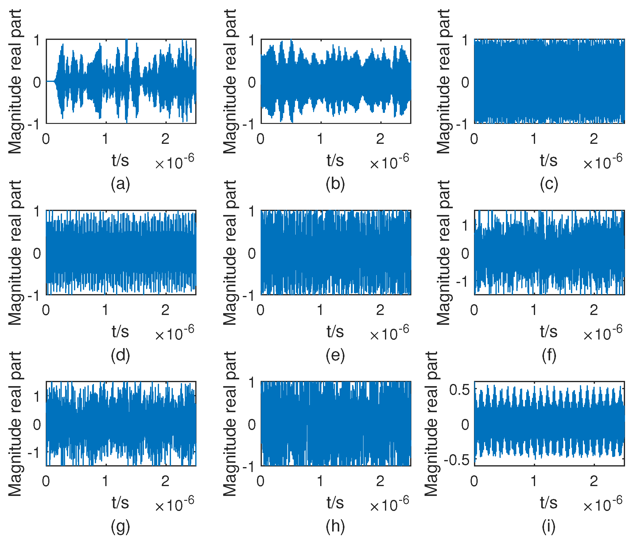
The time-domain waveforms of the nine patterns are shown in Figure 1. As can be seen from the figure, there is little difference in the time domain between the various patterns of suppressed jamming signals, which are more difficult to distinguish manually and are easily disturbed by noise.
3. Proposed Method
Assuming that the dataset of jamming signals received by the radar is , it consists of kinds of patterns of jamming. The subset is composed of samples of kinds of known patterns, while the subset is composed of samples of kinds of unknown patterns. The two subsets are complementary, meaning and . For the known patterns set containing samples of kinds of patterns, where represents a -dimensional vector of the i-th sample, is the label of the sample, and denotes the -dimensional semantic vector describing the features of the sample’s corresponding pattern to be obtained by supervised learning. Similarly, for the unknown patterns dataset consisting of samples of kinds of patterns, , where is the -dimensional feature vector of the i-th sample, represents the label of the sample, and denotes the -dimensional semantic information of the sample’s corresponding pattern.
For the generalized zero-shot learning classification task considered in this paper, the supervised training phase only allows the utilization of dataset of known patterns . However, the objective is to ensure that the model trained in the supervised training phase can accurately classify into the -dimensional space during the unsupervised classification phase.
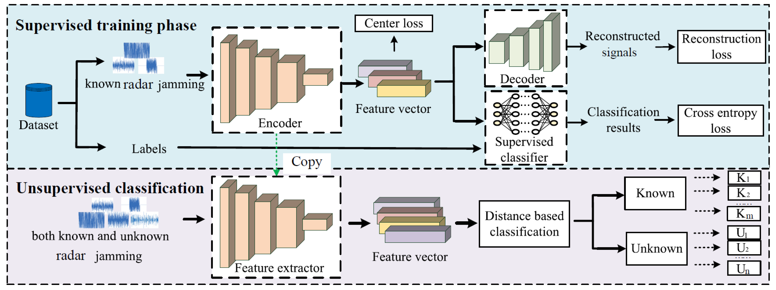
Figure 2 illustrates the network framework of the RCAE-OWR algorithm, which consists of a supervised training phase and an unsupervised classification phase. In the supervised training phase, the residual convolutional autoencoder (RCAE) network is used to extract semantic features of known jamming patterns. Meanwhile, the network is trained using center loss, cross-entropy loss, and reconstruction loss. In [22,37], time-domain signals are directly used as inputs to the network to extract the deep features of different signals, and the simulation results prove that the direct time-domain signal-based recognition methods obtain good recognition performance in terms of accuracy and speed, demonstrating a huge potential for radar signal processing. Motivated by [22,37], in this paper, we also directly feed the IQ data of the jamming signals into the model. Then, after the supervised training, the unsupervised classification phase was entered. At this phase, the parameters of encoder of the RCAE are kept fixed, and both known and unknown jamming samples are input to the encoder to obtain their semantic features. Then, a distance-based discriminative method is employed to achieve open world recognition of radar jamming signals.
3.1. Supervised Training
The supervised training phase mainly consists of an autoencoder network (AE) and a supervised classification network classifier. The autoencoder is divided into two parts: the encoder and the decoder. In the supervised training phase, the focus is on constructing the mapping relationship between the time-domain signal and the semantic features.
3.1.1. Residual Convolutional Autoencoder
Due to the simplicity of the traditional AE structure, this study primarily considers the Residual Convolutional Autoencoder (RCAE). It replaces the fully connected layers in AE with convolutional layers and pooling layers, inheriting the characteristics of an autoencoder. This enables better feature learning and improves the efficiency of feature learning in AE. To prevent degradation in recognition performance, a residual network structure is employed. The input signals are IQ dual-channel data with a length of 512, resulting in a dimension of 2 × 512. Additionally, to maintain the vector dimensions after convolution, we have set the convolution kernel size to 3 × 3, padding = 1 and stride = 1. RCAE is based on the semantic autoencoder (SAE) architecture [31], and SAE enables mapping functions learned from known patterns to be better generalized to unknown patterns, which can effectively resist the domain shift problem [38]. In the encoding process, convolutional operations are used to extract features from input samples and obtain semantic vectors. Then, the decoder utilizes transpose convolution to reconstruct the semantic vectors and restore them to the original inputs.
The basic components of RCAE include the input layer, convolutional layers, semantic layer, deconvolutional layers, and output layer.
The RCAE designed in this paper is illustrated in Figure 3. It replaces the fully connected layers (FC) in the AE with convolutional layers and pooling layers, inheriting the characteristics of the AE for better feature learning. In addition, to prevent degradation of recognition performance, a residual structure is employed. The encoder uses convolutional operations to extract features from the input samples to obtain the semantic vector; the decoder utilizes transposed convolution to reconstruct the semantic vector and reduce it to the original signal.
The basic components of RCAE include: input layer, convolutional layer, semantic layer, deconvolutional layer and output layer.
In the encoding part, the input layer receives the input data and passes it to the encoder. The encoder gradually extracts the semantic features of the input data through multiple convolutional layers and their residual structures, denoted as , where denotes the mapping function of the encoder.
The convolutional layers extract features from the input data using convolutional operations. The data processing can be described as follows:
where is the i-th convolutional kernel matrix, denotes the convolution operation, represents the i-th bias term, represents the activation function. The feature layer integrates the diverse features extracted by the convolutional layers and outputs the semantic vector .
In the decoding part, the semantic feature is up-sampled through transpose convolutional operations, aiming to reconstruct the original signal based on the semantic features. This process is denoted as , where denotes the mapping function of the decoder. Finally, the reconstructed results are outputted through the output layer. The data processing can be described as follows:
where represents the -th convolutional kernel matrix, deconv denotes the transpose convolution operation, represents the i-th bias term.
The training process of aims to minimize the reconstruction error, ensuring the effectiveness of feature extraction. It can be expressed as:
where M represents the number of samples in a batch, is the signal reconstructed by through the RCAE network.
To encourage the feature vectors of the same patterns to be close to their corresponding pattern centers and far from centers of different patterns, a center loss is introduced. During model training, the center loss assigns a center for each jamming pattern. Assuming the input sample is with label , and the center for pattern is denoted as . The center loss can be defined as: 0
During the model iteration process, the selection of pattern center is an important issue. Theoretically, the optimal center for pattern would be the mean of all the feature vectors in that pattern. However, calculating the mean for all samples in each iteration would impose additional computational cost and reduce the efficiency of the model. To address this, the pattern center are initialized randomly, and then updated separately for each batch. The update process is as follows:
where when ; otherwise, it is 0. is the semantic center of at the t-th epoch, is the learning rate.
3.1.2. Supervised Classifier
The encoder, acting as a feature extractor, takes the encoded features and feeds them into a fully connected layer followed by a softmax classifier, which outputs the predicted label. The loss function for this process utilizes cross-entropy between the predicted label and the true label.
where represents the true label in one-hot format, and represents the predicted probability vector.
The reconstruction loss ensures that the reduced-dimensional semantic features are representative, the central loss promotes cohesion among feature vectors of the same jamming pattern, and the cross-entropy loss enhances the discriminative ability of feature vectors among different jamming patterns. To achieve both increased inter-class distance and reduced intra-class distance, a joint loss function is proposed:
where and are constants used to balance the weights of the three loss functions. The detailed gradient of L is shown in Appendix A.
The network parameters during the supervised training phase are updated as shown in Algorithm 1.
| Algorithm 1 Pseudocode for supervised training of RCAE-OWR |
| Input: known jamming patterns dataset and hyperparameter.
Output: Optimal parameters . |
3.2. Unsupervised Classification
After learning the mapping relationship between the original time-domain signals and the semantic feature space in the supervised training phase, this learned relationship can be generalized to the unknown jamming patterns dataset. Finally, the unknown patterns can be recognized and classified using the semantic features. Inspired by [39], a distance-based classification rule is proposed.
3.2.1. Known Jamming Patterns Classification
Sequentially, the known jamming samples from the training set are inputted into the trained RCAE-OWR model to extract semantic features. The semantic center vector corresponding to the k-th known jamming pattern is defined as:
where denotes the semantic feature extracted from the i-th input sample . When a test sample is input, its semantic features are extracted by the encoder, and its Mahalanobis distance to the center vectors of each known jamming pattern is calculated as:
where is the diagonal covariance matrix corresponding to , and is its inverse matrix.
Let . If , then belongs to the known jamming patterns. Here, is a given threshold determined by the criterion [34], where is a coefficient and is the dimension of . In this case, the label of can be determined as follows:
when belongs to the unknown jamming patterns, and its label in this case is described in Section 3.2.2.
3.2.2. Unknown Jamming Patterns Classification
Let represent the dataset of unknown jamming patterns. If , then belongs to the first sample of a new unknown jamming pattern, and its label is . The sample is then recorded in the . If , the following rules are applied to determine whether belongs to a previously recorded unknown jamming pattern or a new unknown jamming pattern. First, let represent the semantic center vector of pattern in the :
where N is the number of patterns that already exist in . denotes the semantics extracted from the j-th unknown pattern sample . Let . If , then belongs to an existing unknown jamming pattern. Here, is a given threshold, where is a coefficient, and are defined as follows:
In this case, the label of can be determined as follows:
Otherwise, belongs to a new unknown jamming pattern, and its label is . The test sample is then recorded in the .
In summary, the recognition rules for the unsupervised classification phase are presented in Algorithm 2.
| Algorithm 2 Pseudocode for unsupervised classification of RCAE-OWR |
| Input: test sample and well-trained weight of Encoder, .
Output: Jamming pattern .
|
4. Performance Evaluation
4.1. Simulation Parameter Settings
The simulations are performed on a PC with an Intel(R) Core(TM) i7-9700 CPU and a GeForce RTX2070s GPU. The deep learning framework PyTorch is used for training and testing the neural network. The RCAE-OWR network is initialized with random weights, and the learning rate is set to 0.001 . The batch size is set to 256, and the number of epochs is set to 250. The values of , and are set to , and 1.5, respectively. Furthermore, grid search is applied to ascertain the optimal hyperparameters. Specifically, we train the model for each possible combination among all the candidate parameters by loop traversal and pick the parameter combination that minimizes the validation set error as the optimal hyperparameters.
4.2. Original Dataset
The jamming signals are generated using MATLAB. The dataset includes the nine kinds of radar active jamming signals mentioned in Section 2.2, with detailed parameters shown in Table 1. The data description is shown in Table 2. Gaussian white noise is added during the simulation, and the JNR ranges from to with a step size of . For each JNR, 1000 samples are generated for each type of radar active jamming signal. In the following experiments, kinds of the jamming patterns will be treated as known jamming, while the remaining kinds of patterns will be treated as unknown jamming.
4.3. Training Process
Firstly, patterns are selected from the original dataset as known patterns, and the remaining patterns are considered unknown patterns. The samples from known patterns are used not only for training the network but also for testing. However, the samples from unknown patterns are exclusively used for testing purposes. To reduce the impact of noise on the training results, during the training phase, only the known pattern samples with a JNR higher than 12 dB are used to train the RCAE-OWR network. For each JNR, 700 samples are randomly selected from the known pattern samples to form the training set, and another 100 samples are randomly chosen to construct the validation set. In the testing phase, a wider range of JNR values is used, namely, JNR = −4–18 dB. For each of the nine jamming patterns, 200 samples are randomly selected at each JNR value to form the test set. It is important to note that the training set, validation set and test set for the known patterns samples are mutually exclusive and do not overlap with each other.
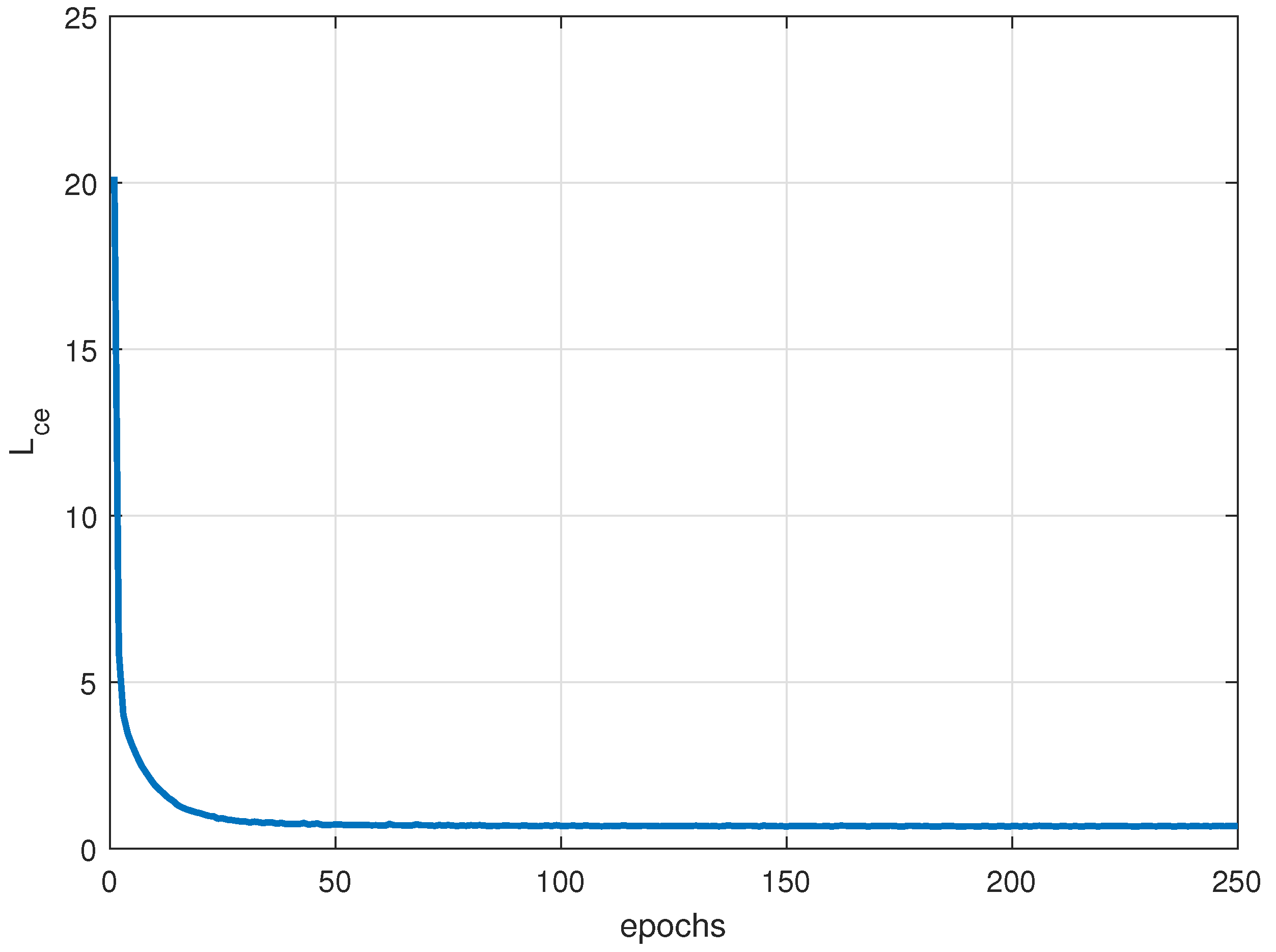
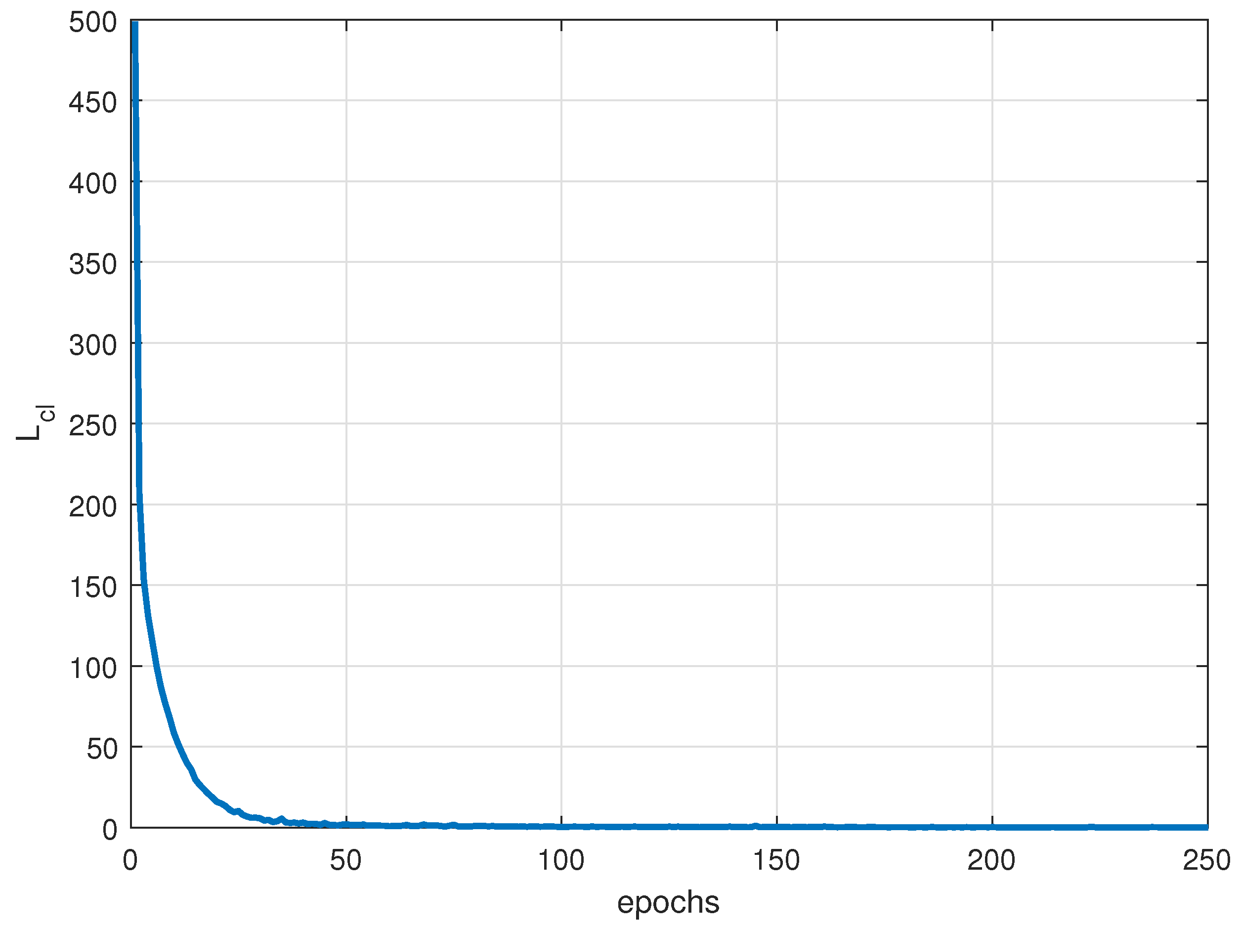
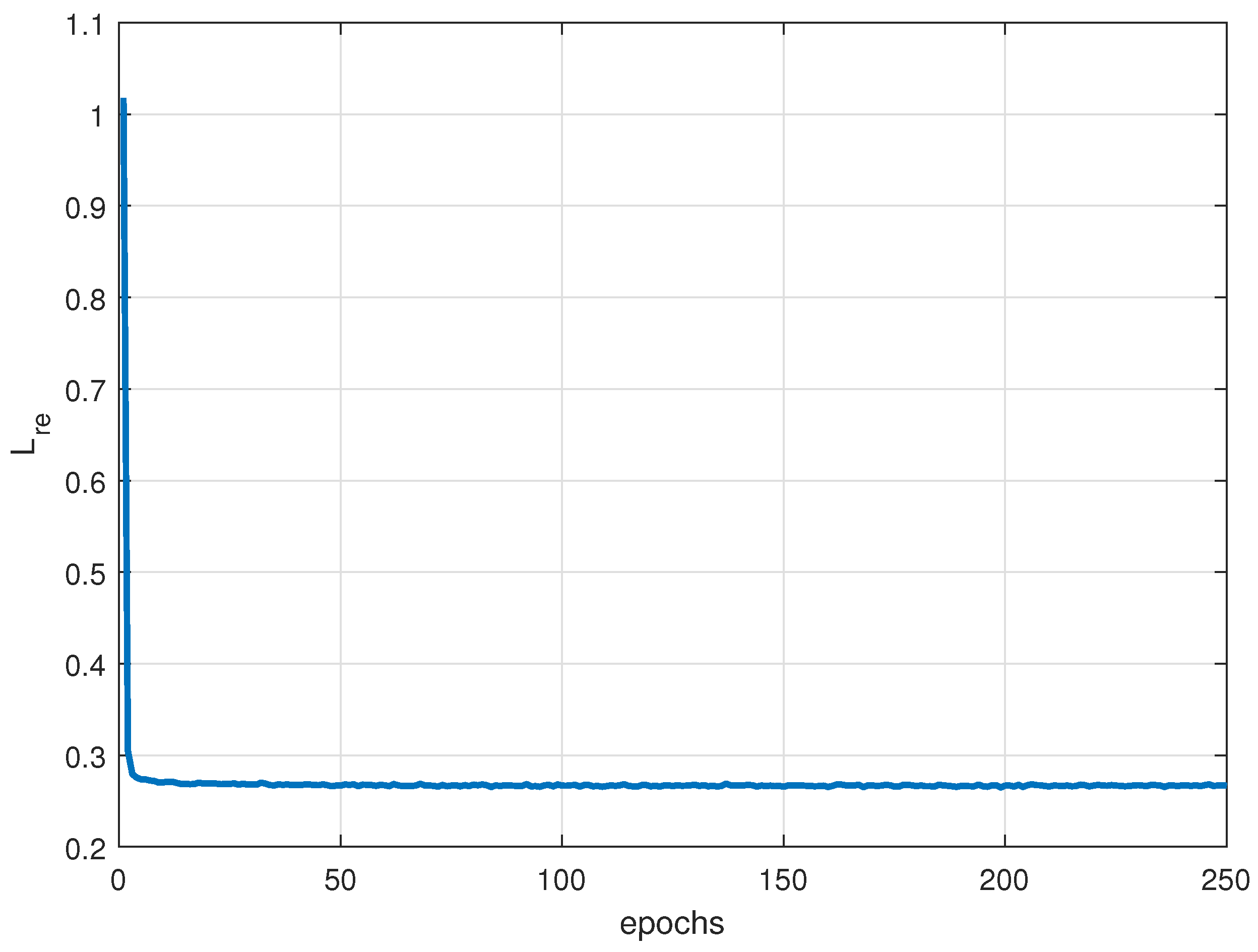
Figure 4, Figure 5 and Figure 6 show the curves of cross-entropy loss , central loss and reconstruction loss of the proposed RACE-OWR algorithm with the number of iterations. It can be seen from the figures that the three losses are gradually decreasing and converging after the epoch exceeds 50, which illustrates the effectiveness and the fast convergence and low complexity of the algorithm. In the convergence stage, the reconstruction loss approaches approximately 0.274, which indicates that the features extracted by the network designed in this paper can effectively represent the original signal and further provide a guarantee for unsupervised classification. The cross-entropy loss converges to 0.82, which contributes to the separation of different patterns, while the central loss converges to 0.12, which contributes to the aggregation of samples from the same pattern.
4.4. Impact of Different Combinations of Unknown Patterns on Classification Performance
In order to investigate the influence of different combinations of unknown patterns on the algorithm’s classification performance, we conducted experiments by randomly selecting two jamming patterns from the dataset as unknown patterns. We define two metrics for evaluation: true known rate (TKR) and true unknown rate (TUR). TKR is calculated as , and is calculated as , where and represent the number of correctly identified samples from known and unknown patterns, respectively, while K and U represent the total number of samples from known and unknown patterns. For ease of comparison, we ensure that the test set’s JNR is consistent with the training set, ranging from 12 to . The experimental results are summarized in Table 3. From the table, it can be observed that at higher JNR values, the algorithm effectively distinguishes between known and unknown patterns, validating the efficacy of our proposed approach. However, under the three combinations tested, neither TKR nor TUR could reach 1. This indicates that some samples from the known patterns are misclassified as unknown, and vice versa.
4.5. Impact of on Algorithm Performance
The value of , which determines the proportion of jamming signal samples classified as known or unknown patterns, is influenced by the value of . In Section 3.2.1, is defined as , where is a constant representing the dimension of the matrix. Therefore, this section investigates the impact of on the algorithm’s performance. Since and cannot both increase with the increase in , a weighted true rate (WTR) [39] is defined to balance these two metrics, i.e., , where is a balancing factor set to 0.5 , indicating equal importance given to and . Figure 7 shows the curves of , , and as varies. It can be observed that as increases, increases while decreases. This is because as increases, the value of increases, so more samples are discriminated as known jamming patterns and fewer samples are discriminated as unknown jamming patterns. The value of initially increases and then decreases with the increase in , reaching its maximum at a value of approximately 0.5∼0.7.
4.6. Ablation Study
In this research, we conduct an ablation study to comprehend the individual contributions of component loss functions in the context of the RCAE-OWR learning model. By systematically eliminating specific component loss functions, we investigate their impact on the overall performance. The experimental findings, as summarized in Table 4, reveal crucial insights into the significance of each loss function. Notably, the removal of (Cross-Entropy Loss) leads to the most substantial performance degradation, resulting in an accuracy of 95.1%. These results underscore the paramount role played by the cross-entropy loss in the learning process, surpassing the influence of the other two component loss functions, namely, and . Furthermore, we observe that the incorporation of Lre enhances the accuracy by 3.3%. This improvement can be attributed to the ability of to preserve essential semantic features, thereby facilitating the differentiation between known and unknown patterns. Additionally, the utilization of the center loss function, yields a minor enhancement in our learning model’s performance.
4.7. Open set Recognition Performance
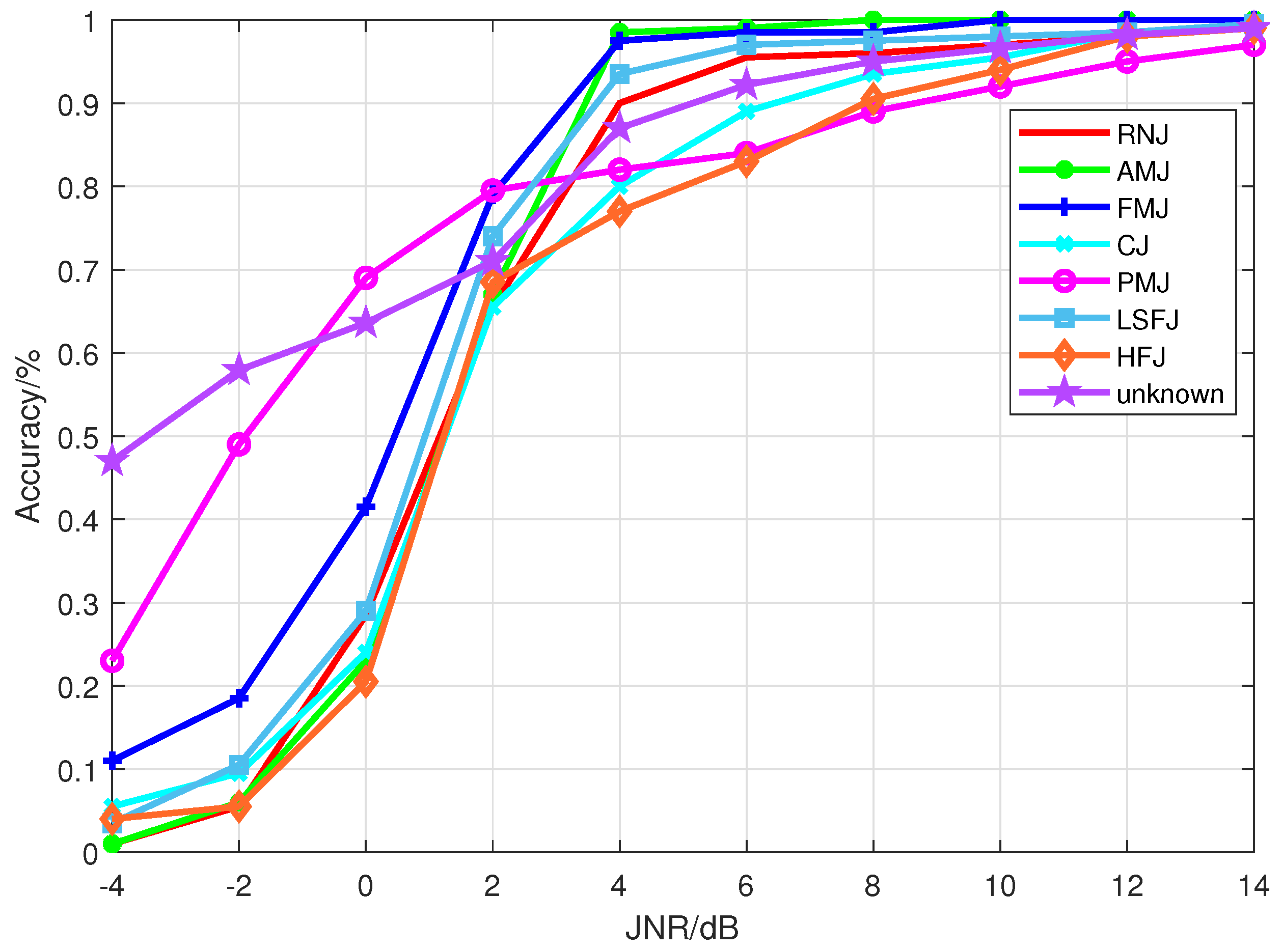
When is set to 7 as well as PGJ and NLSFJ as unknown patterns, the accuracy of the RCAE-OWR algorithm for the seven known jamming patterns and the detection rate for the two unknown jamming patterns are shown in Figure 8. It can be observed that as the JNR increases, the recognition rates for various patterns of jamming also increase.This is because with a higher JNR, the signal becomes cleaner, and the extracted features become more discriminative. When the JNR is below −2 dB, the various jamming signals are submerged in the noise, and the extracted semantic features are not sufficient to separate them. As a result, samples of known jamming patterns are often recognized as samples of unknown jamming patterns, leading to a higher detection rate for unknown jamming patterns compared to known jamming patterns.
Table 5 presents the accuracy of the RCAE-OWR algorithm and the supervised-based algorithm based on seven known jamming patterns when the JNR is set to 10 dB. For a fair comparison, the network structure of the supervised-based algorithm is consistent with the encoder of the RCAE-OWR network in this paper. The difference lies in the fact that the supervised-based algorithm directly outputs the probabilities of the seven jamming patterns as the recognition results, while RCAE-OWR does not have prior knowledge of the specific number of patterns. Therefore, Algorithm 2 is used for jamming pattern recognition in RCAE-OWR. As the supervised-based algorithm is designed for closed-set recognition, it achieves higher detection rates. On the other hand, the RCAE-OWR algorithm is designed for open-set recognition, which means that known jamming patterns can be wrongly recognized as unknown jamming patterns, and unknown jamming patterns can be misclassified as known jamming patterns. As a result, the recognition rate of RCAE-OWR is lower than that of the supervised-based algorithm.
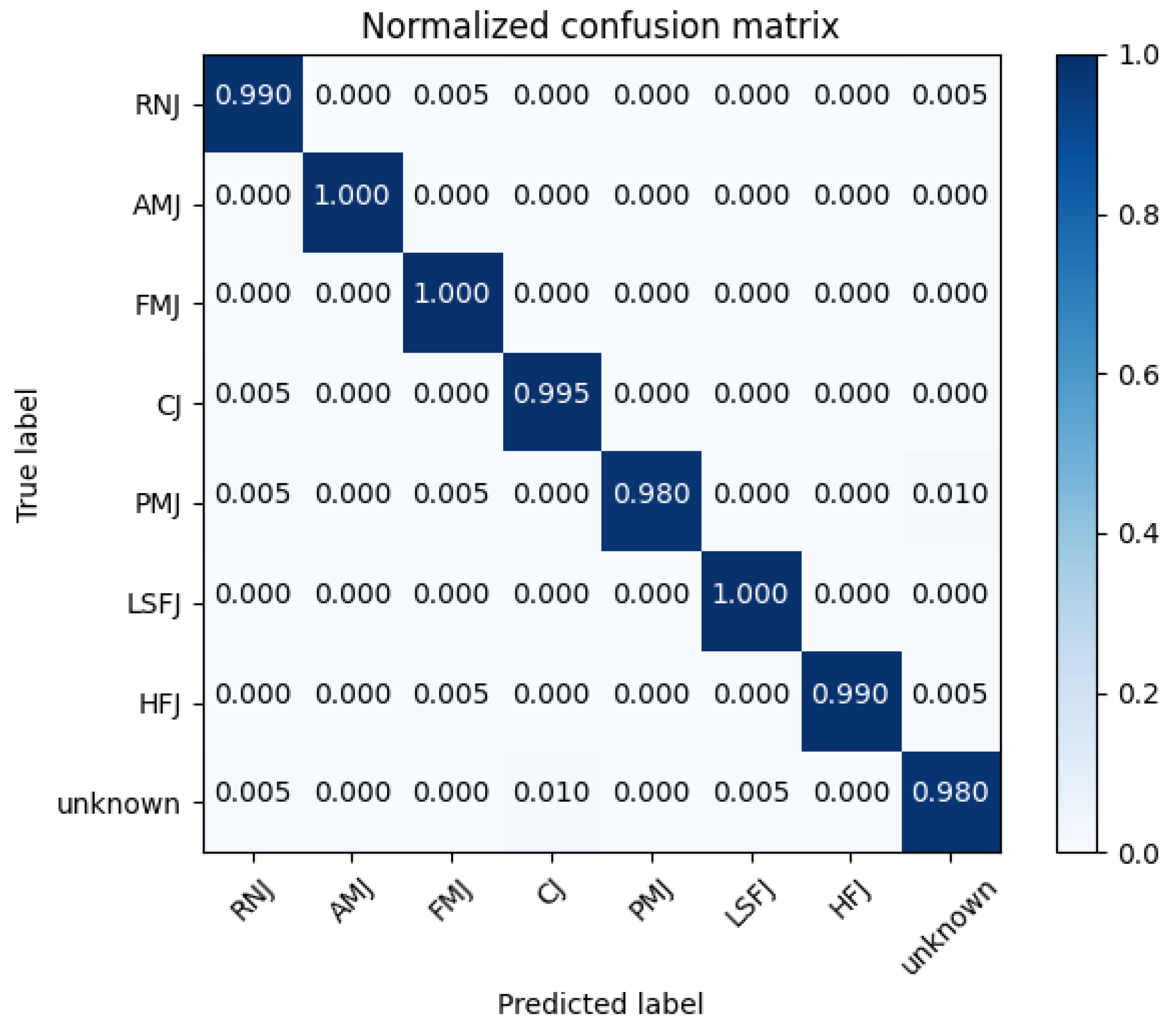
The confusion matrix of RCAE-OWR for known jamming patterns and unknown jamming patterns is shown in Figure 9 when JNR is set to 18 dB. It can be observed from the figure that almost all samples are correctly classified into their respective patterns. This is because with higher levels of jamming, the extracted signal features better represent the original signal, resulting in increased intra-class cohesion and expanded inter-class separation. However, it is also evident that there are cases where known jamming patterns are recognized as unknown jamming patterns, and vice versa. Therefore, our algorithm needs to ensure a high detection rate for unknown jamming patterns while minimizing the impact on the recognition of known jamming patterns.
4.8. Analysis of Unknown Jamming Patterns Recognition Performance in RCAE-OWR
To evaluate the recognition performance of RCAE-OWR for unknown jamming patterns, , , and are introduced as performance metrics [6]. represents the ratio of the number of correctly classified samples to the sum of correctly classified samples and incorrectly classified samples. represents the ratio of the number of correctly classified samples to the total number of samples. is defined as the harmonic mean of and , given by [40].
4.8.1. Performance Comparison of Different Methods
In order to validate the effectiveness of our proposed RCAE-OWR, two other OWR-based methods, IOmSVM [41] and SNN-OWR [35] are implemented for comparison. The features extracted in the IOmSVM method are referenced from [12]. We utilize Openness [42] to measure the complexity of the open world task to describe the weight of the number of unknown patterns. Openness is defined as :
where denotes the number of patterns contained in the training set and denotes the number of patterns contained in the test set. When the Openness is 0 , the task will move to closed-set recognition. In this paper, we set to 9 and keep changing the value of for experiments; score is used to measure the performance of the algorithm and the results are shown in Figure 10. From the figure, it can be seen that as the Openness increases, the classification accuracy of the three methods decreases, which is attributed to the fact that more information about unknown patterns is fed into the model, posing a serious challenge to the classification of the model. Meanwhile, RCAE-OWR has the highest recognition accuracy at the same Openness, e.g., when the Openness is 0.25, the average score of RCAE-OWR is and higher than that of SNN-OWR and IOmSVM, respectively.
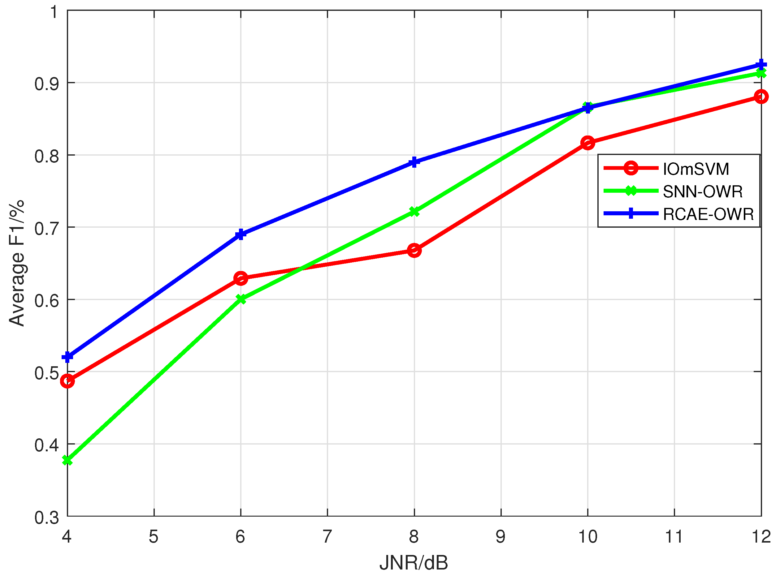
Figure 11 illustrates the performance of the three methods as the JNR varies, with set to 3. Notably, the detection performance of all three methods exhibits improvement as JNR increases, and the differences in scores diminish with higher JNR values. Among the three OWR-based methods, RCAE-OWR stands out with the highest classification accuracy, particularly at low JNR. For instance, when the JNR is 8 dB, the average score of RCAE-OWR surpasses that of SNN-OWR and IOmSVM by 6.85% and 12.23%, respectively.
Table 6 presents the offline training time and online recognition time of the three methods. It can be observed from the table that the IOmSVM method has the shortest training time, and likewise the recognition accuracy is the worst within the three methods. Both SNN-OWR and RCAE-OWR require longer training times; however, once the models are trained effectively, they still achieve real-time jamming recognition.
4.8.2. Impact of Unknown Patterns on RCAE-OWR Performance
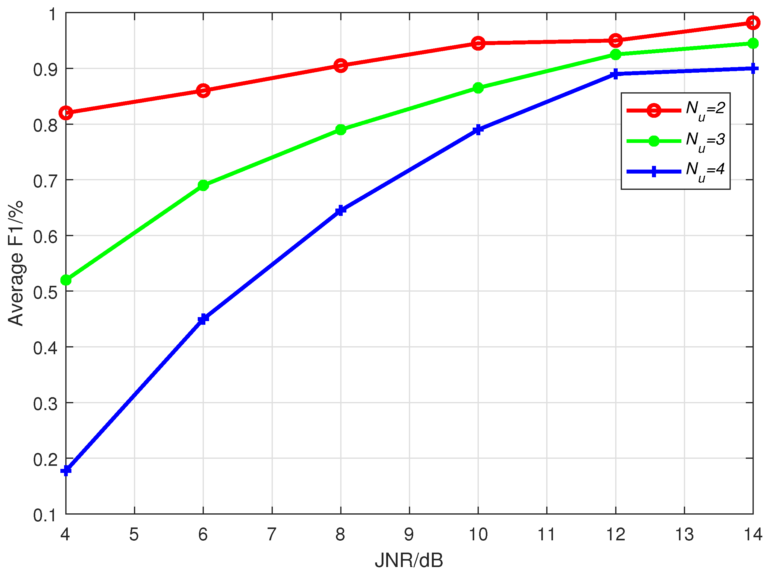
To investigate the influence of the number of unknown jamming patterns on the algorithm’s recognition performance, we randomly selected two, three, four, five and six kinds of patterns out of the nine kinds of jamming patterns as unknown jamming patterns, while the remaining patterns were considered known jamming patterns. The experimental results are presented in Table 7, with JNR set to . From the table, it can be observed that as the number of unknown jamming patterns decreases, the algorithm’s detection performance improves, as indicated by an increase in the score. For example, when the number of unknown jamming patterns is reduced from four to two, the average score increases by 0.070. However, when the number of unknown patterns surpasses the number of known patterns, it poses a challenge to the algorithm’s detection performance. For example, when increasing the number of unknown patterns from four to five, the average score decreases by 0.174.
4.8.3. Recognition Performance of RCAE-OWR for Unknown Jamming Patterns
The recognition rates of RCAE-OWR for unknown jamming patterns with JNR of 4∼14 dB are shown in Figure 12. It can be observed from the graph that when the number of unknown jamming patterns is fixed, the average score increases with the increase in JNR. This is because at lower JNR levels, a large number of known jamming patterns are incorrectly classified as unknown, resulting in poor classification performance. As the JNR increases, the characteristics of different jamming signals become more distinct, and the samples of known patterns wrongly classified as unknown patterns decrease, leading to improved performance in classifying unknown patterns. Additionally, at lower JNR levels, there is a significant difference in the average score among the three different jamming patterns. However, as the JNR increases, this difference decreases. For example, at JNR = 4 dB, the average score for two unknown patterns is 0.3 and 0.65 higher than that for three and four unknown patterns, respectively. At JNR = 10 dB, the average score for two unknown patterns is 0.08 and 0.15 higher than that for three and four unknown patterns, respectively. This also highlights the importance of improving the JNR of the dataset as a prerequisite and guarantee for open world recognition of radar jamming signals.
4.8.4. Performance of RCAE-OWR for Unknown Patterns under Different Combinations
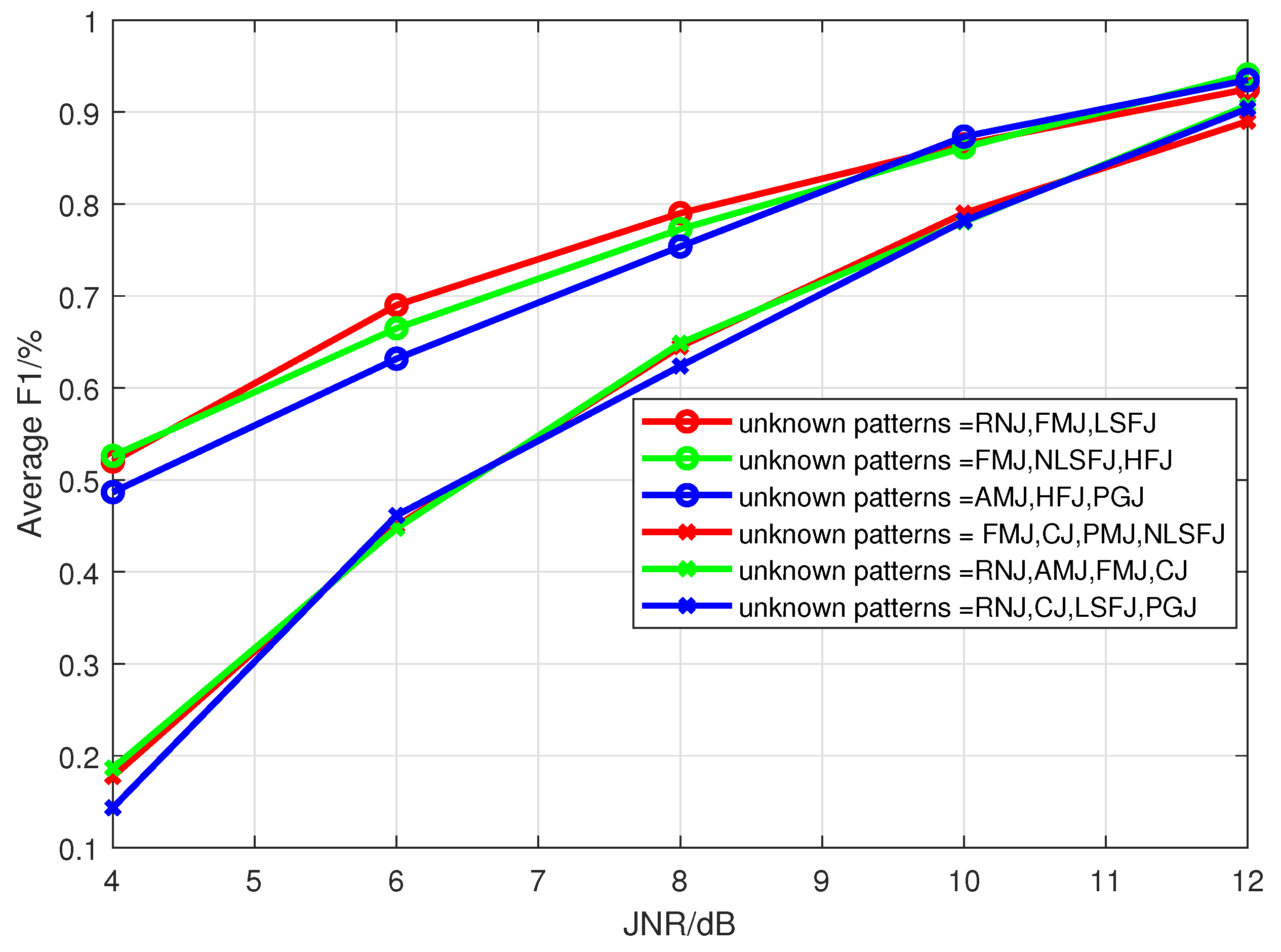
To investigate the influence of JNR on the algorithm’s performance with varying combinations of unknown patterns, we randomly extract three or four kinds of signals from the dataset to form the unknown patterns set, while the remaining are considered as known patterns for experimental evaluation. The results of these experiments are presented in Figure 13. From the figure, it can be seen that as the JNR increases, the overall classification accuracy also improves; this is because as the JNR increases, the signal is less affected by noise and is more discriminative. Notably, when the number of unknown patterns is fixed, the classification accuracy consistently increases with higher JNR values. Additionally, regardless of the specific combination of unknown patterns data sets, the classification accuracy exhibits minimal variation under the same JNR condition, highlighting the robustness of the RCAE-OWR algorithm.
5. Conclusions
In this study, we addressed the problem of open world recognition for radar jamming signals. Leveraging the idea of zero-shot learning, we proposed an open world recognition method called RCAE-OWR based on residual autoencoders. This method utilizes the features extracted by the encoder network to form the semantic centers of known jamming patterns. Then, a distance-based approach is proposed to classify known and unknown jamming patterns. Experimental results demonstrate that the RCAE-OWR algorithm can effectively recognize unknown jamming patterns, especially under high JNR. Although the proposed RCAE-OWR algorithm has demonstrated excellent classification performance in suppression jamming signals, there are still some limitations and drawbacks to address. For instance, this paper focused only on common jamming signals, while there are other jamming patterns, such as agile noise jamming and deceptive jamming. In the future, these patterns should be incorporated into our method. Additionally, deep learning has been widely applied to intelligent radar jamming signal recognition with a balanced training set. However, in most cases, an imbalanced training set is inevitable. Therefore, considering open world recognition of radar jamming under class-imbalanced conditions will be a challenging yet valuable task in future research.
Author Contributions
Conceptualization Z.Z. and Y.Z.; methodology, Y.Z. and Z.Z.; software, Y.B. and Y.Z.; validation, Z.Z.; formal analysis, Z.Z.; investigation, Z.Z. and Y.Z.; resources, Z.Z.; data curation, Y.B.; writing—original draft preparation, Y.Z.; writing—review and editing, Y.B. and Y.Z.; visualization, Z.Z.; supervision, Z.Z.; project administration, Y.Z.; funding acquisition, Z.Z. All authors have read and agreed to the published version of the manuscript.
Funding
This work was supported by the State Key Program of National Natural Science of China (Grant No. U19B2016) and Zhejiang Provincial Key Lab of Data Storage and Transmission Technology, Hangzhou Dianzi University.
Acknowledgments
The authors would like to thank an Editor who handled the manuscript and the anonymous reviewers for their valuable comments and suggestions.
Conflicts of Interest
The authors declare no conflict of interest.
Appendix A
Appendix A.1
Lemma A1.
Assuming the and are gradients of and , respectively, then there is:
Proof.
because can be notated as:
□
Notice that , where , Let denote the output vector of the last layer of the network. After softmax operation, yields . That is, . where represents the softmax operation, and and are the j-th elements of and , respectively. According to the chain derivative rule:
We have:
Simplify to get:
Hence, can be rewritten as:
therefore, according to , we have:
Similarly, , and , we have:
Similarly,
In summary, it can be concluded that:
References
- Du, C.; Cong, Y.; Zhang, L.; Guo, D.; Wei, S. A Practical Deceptive Jamming Method Based on Vulnerable Location Awareness Adversarial Attack for Radar HRRP Target Recognition. IEEE Trans. Inf. Forensics Secur. 2022, 17, 2410–2424. [Google Scholar] [CrossRef]
- Xu, H.; Quan, Y.; Zhou, X.; Chen, H.; Cui, T.J. A Novel Approach for Radar Passive Jamming Based on Multiphase Coding Rapid Modulation. IEEE Trans. Geosci. Remote Sens. 2023, 61, 1–14. [Google Scholar] [CrossRef]
- Liu, Z.; Zhao, S. Unsupervised Clustering Method to Discriminate Dense Deception Jamming for Surveillance Radar. IEEE Sensors Lett. 2021, 5, 1–4. [Google Scholar] [CrossRef]
- Lv, Q.; Quan, Y.; Feng, W.; Sha, M.; Dong, S.; Xing, M. Radar Deception Jamming Recognition Based on Weighted Ensemble CNN With Transfer Learning. IEEE Trans. Geosci. Remote Sens. 2022, 17, 1–11. [Google Scholar] [CrossRef]
- Hua, Q.; Zhang, Y.; Wei, C.; Ji, Z.; Jiang, Y.; Wang, Y.; Xu, D. A Self-Supervised Method Based on CV-MUNet++ for Active Jamming Suppression in SAR Images. IEEE Trans. Geosci. Remote Sens. 2023, 61, 1–16. [Google Scholar] [CrossRef]
- Luo, Z.; Cao, Y.; Yeo, T.S.; Wang, Y.; Wang, F. Few-Shot Radar Jamming Recognition Network via Time-Frequency Self-Attention and Global Knowledge Distillation. IEEE Trans. Geosci. Remote Sens. 2023, 61, 1–12. [Google Scholar] [CrossRef]
- Huang, S.; Feng, Z.; Zhang, Y.; Zhang, K.; Li, W. Feature based modulation classification using multiple cumulants and antenna array. In Proceedings of the 2016 IEEE Wireless Communications and Networking Conference, Doha, Qatar, 3–6 April 2016; pp. 1–5. [Google Scholar]
- Chen, T.; Gao, S.; Zheng, S.; Yu, S.; Xuan, Q.; Lou, C.; Yang, X. EMD and VMD Empowered Deep Learning for Radio Modulation Recognition. IEEE Trans. Cogn. Commun. Netw. 2023, 9, 43–57. [Google Scholar] [CrossRef]
- Zhu, F.; Jiang, Q.Q.; Lin, C.; Xiao, Y. Typical wide band EMI identification based on support vector machine. Syst. Eng. Electron. 2021, 43, 2400–2406. [Google Scholar]
- Lu, Y.; Li, S. CFAR detection of DRFM deception jamming based on singular spectrum analysis. In Proceedings of the 2017 IEEE International Conference on Signal Processing, Communications and Computing (ICSPCC), Xiamen, China, 22–25 October 2018; pp. 1–6. [Google Scholar]
- Yang, S.; Tian, B.; Zhou, R. A jamming identification method against radar deception based on bispectrum analysis and fractal dimension. J. Xian Jiaotong Univ. 2016, 50, 128–135. [Google Scholar]
- Xu, C.; Yu, L.; Wei, Y.; Tong, P. Research on Active Jamming Recognition in Complex Electromagnetic Environment. In Proceedings of the 2019 IEEE International Conference on Signal, Information and Data Processing (ICSIDP), Chongqing, China, 11–13 December 2019; pp. 1–5. [Google Scholar]
- Wei, Y.; Li, Y.; Zhang, J.; Tong, P. Radar Jamming Recognition Method Based on Fuzzy Clustering Decision Tree. In Proceedings of the 2019 IEEE International Conference on Signal, Information and Data Processing (ICSIDP), Chongqing, China, 11–13 December 2019; pp. 1–5. [Google Scholar]
- Yu, Y.; Li, J.; Li, J.; Xia, Y.; Ding, Z.; Samali, B. Automated damage diagnosis of concrete jack arch beam using optimized deep stacked autoencoders and multi-sensor fusion. Dev. Built Environ. 2023, 14, 100128. [Google Scholar] [CrossRef]
- Zhang, Y.; Zhao, Z. Limited Data Spectrum Sensing Based on Semi-Supervised Deep Neural Network. IEEE Access 2021, 9, 1813–1817. [Google Scholar] [CrossRef]
- Zhang, Y.P.; Zhao, Z.J. Semi-supervised deep learning using pseudo labels for spectrum sensing. J. Nonlinear Convex Anal. 2022, 23, 1913–1929. [Google Scholar]
- Yu, Y.; Hoshyar, A.N.; Samali, B.; Zhang, G.; Rashidi, M.; Mohammadi, M. Corrosion and coating defect assessment of coal handling and preparation plants (CHPP) using an ensemble of deep convolutional neural networks and decision-level data fusion. Neural Comput. Appl. 2023, 35, 18697–18718. [Google Scholar] [CrossRef]
- Lv, Q.; Quan, Y.; Sha, M.; Feng, W.; Xing, M. Deep Neural Network-Based Interrupted Sampling Deceptive Jamming Countermeasure Method. IEEE J. Sel. Top. Appl. Earth Obs. Remote Sens. 2022, 15, 9073–9085. [Google Scholar] [CrossRef]
- Zhao, Q.; Liu, Y.; Cai, L.; Lu, Y. Research on electronic jamming identification based on CNN. In Proceedings of the 2019 IEEE International Conference on Signal, Information and Data Processing (ICSIDP), Chongqing, China, 11–13 December 2019. [Google Scholar]
- Li, M.; Ren, Q.; Wu, J. Interference classification and identification of TDCS based on improved convolutional neural network. J. Phys. Conf. Ser. 2020, 16, 121–155. [Google Scholar] [CrossRef]
- Liu, Q.; Zhang, W. Deep learning and recognition of radar jamming based on CNN. In Proceedings of the 2019 12th International Symposium on Computational Intelligence and Design (ISCID), Hangzhou, China, 14–15 December 2019; pp. 208–212. [Google Scholar]
- Shao, G.; Chen, Y.; Wei, Y. Convolutional neural network-based radar jamming signal classification with sufficient and limited samples. IEEE Access 2020, 8, 80588–80598. [Google Scholar] [CrossRef]
- Shao, G.; Chen, Y.; Wei, Y. Deep fusion for radar jamming signal classification based on CNN. IEEE Access 2020, 8, 117236–117244. [Google Scholar] [CrossRef]
- Tian, X.; Chen, B.; Zhang, Z. Multiresolution Jamming Recognition with Few-shot Learning. In Proceedings of the 2021 CIE International Conference on Radar (Radar), Haikou, Hainan, China, 15–19 December 2021; pp. 2267–2271. [Google Scholar]
- Luo, H.; Liu, J.; Wu, S.; Nie, Z. A Semi-Supervised Deception Jamming Discrimination Method. In Proceedings of the 2021 IEEE 7th International Conference on Cloud Computing and Intelligent Systems (CCIS), Xi’an, China, 7–8 November 2021; pp. 428–432. [Google Scholar]
- Zhou, Y.; Shang, S.; Song, X.; Zhang, S.; You, T.; Zhang, L. Intelligent Radar Jamming Recognition in Open Set Environment Based on Deep Learning Networks. Remote Sens. 2022, 14, 2410–2424. [Google Scholar] [CrossRef]
- Wang, L.; Yang, X.; Tan, H.; Bai, X.; Zhou, F. Few-Shot Class-Incremental SAR Target Recognition Based on Hierarchical Embedding and Incremental Evolutionary Network. IEEE Trans. Geosci. Remote Sens. 2023, 61, 1–11. [Google Scholar] [CrossRef]
- Wei, Q.R.; He, H.; Zhao, Y.; Li, J.A. Learn to Recognize Unknown SAR Targets From Reflection Similarity. IEEE Geosci. Remote Sens. Lett. 2022, 19, 1–5. [Google Scholar] [CrossRef]
- Song, Q.; Chen, H.; Xu, F.; Cui, T.J. EM Simulation-Aided Zero-Shot Learning for SAR Automatic Target Recognition. IEEE Geosci. Remote Sens. Lett. 2020, 17, 1092–1096. [Google Scholar] [CrossRef]
- Bernardino, R.P.; Torr, P.H.S. An embarrassingly simple approach to zero-shot learning. In Proceedings of the 32nd international conference on Machine learning (ICML’15), Lille, France, 6–11 July 2015. [Google Scholar]
- Kodirov, E.; Xiang, T.; Gong, S. Semantic Autoencoder for Zero-Shot Learning. In Proceedings of the 2017 IEEE Conference on Computer Vision and Pattern Recognition (CVPR), Honolulu, HI, USA, 21–26 July 2017; pp. 4447–4456. [Google Scholar]
- Zhang, L.; Xiang, T.; Gong, S. Learning a Deep Embedding Model for Zero-Shot Learning. In Proceedings of the 2017 IEEE Conference on Computer Vision and Pattern Recognition (CVPR), Honolulu, HI, USA, 21–26 July 2017; pp. 3010–3019. [Google Scholar]
- Ma, B.J.; Qi, J.; Su, H.Y.; Zhang, X.F. One-dimensional Radar Active Jamming Signal Recognition Method Based on Bayesian Deep Learning. Signal Process. 2023, 39, 235–243. [Google Scholar]
- Qu, Q.; Wei, S.; Liu, S.; Liang, J.; Shi, J. JRNet: Jamming Recognition Networks for Radar Compound Suppression Jamming Signals. IEEE Trans. Veh. Technol. 2020, 69, 15035–15045. [Google Scholar] [CrossRef]
- Tang, Y.; Zhao, Z.; Chen, J.; Zheng, S.; Ye, X.; Lou, C.; Yang, X. Open world recognition of communication jamming signals. China Commun. 2023, 20, 199–214. [Google Scholar] [CrossRef]
- Wang, J.Q. Study and Implementation of Radar Active Jamming Type Discrimination. Master’s Thesis, Xidian University, Xi’an, China, 2014. [Google Scholar]
- Zhang, H.; Yu, L.; Chen, Y.; Wei, Y. Fast Complex-Valued CNN for Radar Jamming Signal Recognition. Remote Sens. 2021, 13, 2867. [Google Scholar] [CrossRef]
- Fu, Y.; Hospedales, T.M.; Xiang, T.; Gong, S. Trans-ductive multi-view zero-shot learning. IEEE Tran. PAMI 2015, 37, 2332–2345. [Google Scholar] [CrossRef]
- Dong, Y.; Jiang, X.; Zhou, H.; Lin, Y.; Shi, Q. SR2CNN: Zero-Shot Learning for Signal Recognition. IEEE Trans. Signal Process. 2021, 69, 2316–2329. [Google Scholar] [CrossRef]
- Yang, L.; Li, Q.; Shao, H.Z. An Open Set Recognition Algorithm of Electromagnetic Target Based on Metric Learning and Feature Subspace Projection. Acta Electron. Sin. 2022, 17, 1310–1318. [Google Scholar]
- Jleed, H.; Martin, B. Incremental multiclass open-set audio recognition. Int. J. Adv. Intell. Inform. 2022, 8, 251–270. [Google Scholar] [CrossRef]
- Geng, X.; Dong, G.; Xia, Z.; Liu, H. SAR Target Recognition via Random Sampling Combination in Open-World Environments. IEEE J. Sel. Top. Appl. Earth Obs. Remote Sens. 2023, 16, 331–343. [Google Scholar] [CrossRef]
Figure 1.
Time-domain waveforms of nine patterns of radar jamming signals. From (a) to (i): (a) RNJ, (b) AMJ, (c) FMJ, (d) CJ, (e) PMJ, (f) LSFJ, (g) NLSFJ, (h) HFJ, (i) PGJ.
Figure 1.
Time-domain waveforms of nine patterns of radar jamming signals. From (a) to (i): (a) RNJ, (b) AMJ, (c) FMJ, (d) CJ, (e) PMJ, (f) LSFJ, (g) NLSFJ, (h) HFJ, (i) PGJ.

Figure 2.
Radar jamming recognition framework of RCAE-OWR.

Figure 3.
Residual Convolutional Autoencoder Network Structure.

Figure 4.
Cross-entropy loss.

Figure 5.
Center loss.

Figure 6.
Reconstruction loss.

Figure 7.
The impact of on recognition rate.

Figure 8.
Open set recognition of RCAE-OWR.

Figure 9.
RCAE-OWR open set recognition results when JNR = 18 dB.

Figure 10.
scores against varying Openness under different methods.

Figure 11.
scores against JNR under different methods.

Figure 12.
Recognition performance of RCAE-OWR for different unknown jamming patterns.

Figure 13.
Performance under different unknown patterns.


Table 1.
Nine kinds of Radar Active Jamming Parameter Settings.
| Jamming Pattern | Parameter Description |
|---|---|
| RNJ | Carrier frequency: 60∼110 MHz. |
| AMJ | Carrier frequency: 60∼110 MHz, bandwidth: 5∼10 MHz, K: 0.1∼0.9 |
| FMJ | Carrier frequency: 60∼110 MHz, bandwidth: 5∼10 MHz, K: 0.1∼0.9 |
| CJ | Carrier frequency: 60∼110 MHz, bandwidth: 5∼10 MHz, number of bands: 2∼4 |
| PMJ | Carrier frequency: 60∼110 MHz, bandwidth: 5∼10 MHz, K: 0.1∼0.9 |
| LSFJ | Starting frequency: 1∼10 MHz, ending frequency: 50∼100 MHz. |
| NLSFJ | Starting frequency: 1∼10 MHz, ending frequency: 50∼100 MHz. |
| HFJ | = 20, : [10, 100] MHz, : 32∼64 s |
| PGJ | Pulse period T: [2.5, 10] s . Duty cycle: [1/8, 1/2] |
Table 2.
The original dataset.
| Total Samples | Samples of Each Pattern | Samples Each JNR | Feature Dimension | Patterns |
|---|---|---|---|---|
| 108,000 | 12,000 | 1000 | 2 × 512 | 9 |
| patterns | ||||
| RNJ, AMJ, FMJ, CJ, PMJ, LSFJ, NLSFJ, HFJ, PGJ | ||||
| number of JNR values | JNR values | |||
| 12 | −4, −2, 0, 2, 4, 6, 8, 10, 12, 14, 16, 18 | |||
Table 3.
Performance with different unknown pattern combinations.
| Indicator | Unknown Patterns | ||
|---|---|---|---|
| RNJ, HFJ | AMJ, PGJ | RNJ, NLSFJ | |
| Average accuracy | 0.957 | 0.965 | 0.978 |
| TKR | 0.966 | 0.982 | 0.994 |
| TUR | 0.999 | 0.999 | 0.995 |
Table 4.
Ablation study on RCAE-OWR. : cross entropy loss. : center loss. : reconstruction loss.
| Variant | True Rate |
|---|---|
| RCAE-OWR(, and ) | 0.995 |
| without | 0.951 |
| without | 0.982 |
| without | 0.962 |
Table 5.
Comparison of detection performance between two algorithms.
| Method | RNJ | AMJ | FMJ | CJ | PMJ | LSFJ | HFJ |
|---|---|---|---|---|---|---|---|
| supervised | 98% | 100% | 99% | 95% | 92% | 98% | 95% |
| RCAE-OWR | 96% | 100% | 98.5% | 93.5% | 89% | 97.5% | 90.5% |
Table 6.
Runtime (in seconds) of different methods.
| Method | Offline Training | Online Recognition |
|---|---|---|
| IOmSVM | 753 | 0.0075 |
| SNN-OWR | 1506 | 0.0071 |
| RCAE-OWR | 1427 | 0.0062 |
Table 7.
Effect of Unknown jamming patterns on RCAE-OWR Performance.
| Number of Patterns | Pattern | |||
|---|---|---|---|---|
| 2 | Pattern 1 | 0.941 | 0.964 | 0.952 |
| Pattern 2 | 0.979 | 0.940 | 0.959 | |
| 3 | Pattern 1 | 0.916 | 0.940 | 0.927 |
| Pattern 2 | 0.929 | 0.928 | 0.928 | |
| Pattern 3 | 0.922 | 0.900 | 0.910 | |
| 4 | Pattern 1 | 0.861 | 0.930 | 0.894 |
| Pattern 2 | 0.907 | 0.920 | 0.913 | |
| Pattern 3 | 0.912 | 0.820 | 0.863 | |
| Pattern 4 | 0.909 | 0.841 | 0.873 | |
| 5 | Pattern 1 | 0.841 | 0.724 | 0.778 |
| Pattern 2 | 0.781 | 0.696 | 0736 | |
| Pattern 3 | 0.701 | 0.680 | 0.690 | |
| Pattern 4 | 0.623 | 0.713 | 0.663 | |
| Pattern 5 | 0.542 | 0.692 | 0.692 | |
| 6 | Pattern 1 | 0.779 | 0.598 | 0.677 |
| Pattern 2 | 0.712 | 0.545 | 0.613 | |
| Pattern 3 | 0.603 | 0.536 | 0.567 | |
| Pattern 4 | 0.481 | 0.533 | 0.505 | |
| Pattern 5 | 0.365 | 0.452 | 0.402 | |
| Pattern 6 | 0.243 | 0.405 | 0.301 |
Disclaimer/Publisher’s Note: The statements, opinions and data contained in all publications are solely those of the individual author(s) and contributor(s) and not of MDPI and/or the editor(s). MDPI and/or the editor(s) disclaim responsibility for any injury to people or property resulting from any ideas, methods, instructions or products referred to in the content. |
© 2023 by the authors. Licensee MDPI, Basel, Switzerland. This article is an open access article distributed under the terms and conditions of the Creative Commons Attribution (CC BY) license (https://creativecommons.org/licenses/by/4.0/).
Share and Cite
MDPI and ACS Style
Zhang, Y.; Zhao, Z.; Bu, Y. Radar Active Jamming Recognition under Open World Setting. Remote Sens. 2023, 15, 4107. https://0-doi-org.brum.beds.ac.uk/10.3390/rs15164107
AMA Style
Zhang Y, Zhao Z, Bu Y. Radar Active Jamming Recognition under Open World Setting. Remote Sensing. 2023; 15(16):4107. https://0-doi-org.brum.beds.ac.uk/10.3390/rs15164107
Chicago/Turabian StyleZhang, Yupei, Zhijin Zhao, and Yi Bu. 2023. "Radar Active Jamming Recognition under Open World Setting" Remote Sensing 15, no. 16: 4107. https://0-doi-org.brum.beds.ac.uk/10.3390/rs15164107
Note that from the first issue of 2016, this journal uses article numbers instead of page numbers. See further details here.