Article

A Data-Fusion Approach to Assessing the Contribution of Wildland Fire Smoke to Fine Particulate Matter in California

1
Department of Statistics, North Carolina State University, Raleigh, NC 27695, USA
2
INIBIOMA-CONICET, National University of Comahue, Bariloche R8400, Rio Negro, Argentina
3
Department of Statistical Science, University of Toronto, Toronto, ON M5R OA3, Canada
4
Department of Statistics, Colorado State University, Fort Collins, CO 80523, USA
5
US Environmental Protection Agency, Durham, NC 27709, USA
*
Author to whom correspondence should be addressed.
Remote Sens. 2023, 15(17), 4246; https://0-doi-org.brum.beds.ac.uk/10.3390/rs15174246
Submission received: 30 June 2023 / Revised: 14 August 2023 / Accepted: 21 August 2023 / Published: 29 August 2023

Abstract

:
The escalating frequency and severity of global wildfires necessitate an in-depth understanding and monitoring of wildfire smoke impacts, specifically its contribution to fine particulate matter (PM 2.5 ). We propose a data-fusion method to study wildfire contribution to PM 2.5 using satellite-derived smoke plume indicators and PM 2.5 monitoring data. Our study incorporates two types of monitoring data, the high-quality but sparse Air Quality System (AQS) stations and the abundant but less accurate PurpleAir (PA) sensors that are gaining popularity among citizen scientists. We propose a multi-resolution spatiotemporal model specified in the spectral domain to calibrate the PA sensors against accurate AQS measurements, and leverage the two networks to estimate wildfire contribution to PM 2.5 in California in 2020 and 2021. A Bayesian approach is taken to incorporate all uncertainties and our prior intuition that the dependence between networks, as well as the accuracy of PA network, vary by frequency. We find that 1% to 3% increase in PM 2.5 concentration due to wildfire smoke, and that leveraging PA sensors improves accuracy.

1. Introduction

Airborne particles are a serious environmental health risk globally, contributing in excess of 7 million premature deaths each year [1]. Fine particulate matter (PM 2.5 , particles with a diameter of less than 2.5 micrometers) has been causally linked to cardiovascular morbidity and mortality [2] and are therefore regulated under the provisions of the Clean Air Act [3] to protect human health and wellbeing. As a result, the emissions of PM 2.5 from many antropogenic sources, such as transpiration and industry, have been on a steady decline [4] and wildfires have become the single largest source [5], potentially off setting reduction in emissions from other sources.
High concentrations of fine particles and gasses found in smoke have also produced alarming impacts on health [6,7]. During peak wildfire seasons, smoke exposure can exacerbate health problems, causing a spike in emergency department visits [8]. In an epidemiological study of health impacts by Thilakaratne et al., they estimated that 2.2% of annual respiratory health burden, or 92 ED visits per 100,000 people, is attributed to ambient particulate matter and that wildfire days account for over 15% of that burden [9]. However, providing a definite answer as to how much of particle pollution can be attributed to wildfires remains a challenging problem because instruments measure a total ambient concentration which is composed of natural, anthropogenic, and wildfire sources.
Previous research [10,11,12] has studied the contribution of wildfires on PM 2.5 concentrations by integrating remote sensing data on the location and extend of smoke plumes and PM 2.5 readings from Air Quality System (AQS) monitors deployed by the Environmental Protection Agency (EPA). These studies revealed that wildfires contribute to 40% of unhealthy days and substantially increase PM 2.5 concentrations [13,14]. Wildfire smoke impacts are dynamic and often affect areas without a monitoring station, as AQS monitors have limited spatial coverage due to the high cost and difficulty in installation. It is important to make air quality information available to the public quickly during wildfires, therefore AQS alone provides insufficient data source for monitoring wildfire emissions.
The increased incidence of days with poor air quality due to wildfires has created a demand and public interest for monitoring particulate pollution. Perhaps the most prevalent sensors are PurpleAir (PA), which are installed by members of the public, providing a real-time (every two minutes) monitoring of PM 2.5 with extensive spatial coverage [15]. However, it is known that PA sensors are less reliable compared to the AQS, and thus correction to the sensor readings is needed [16,17]. Barkjohn et al. developed a correction equation using meteorological conditions including relative humidity and temperature, as both measurements affect the accuracy of the instrument [15]; however, this calibration is developed for a US-wide correction and without smoke impacts. Another simple linear correction model under smoke impacted conditions was proposed by Holder et al. in [18]. As the sensor performance can be affected by geographic and environmental conditions, it is more reasonable to relax the assumption of a constant spatially varying bias, but rather capture the spatiotemporally varying bias.
Previous studies have either separated anthropogenic PM 2.5 from smoke emissions using chemical transport models or by subtracting out historically observed averages [19]. However, neither approach provides a definite answer as to how much of particle pollution can be attributed to wildfires. Data fusion is a widely used method that integrates information from different types of sensors to provide a robust and complete description of a process of interest [20,21]. It has been used extensively to estimate spatially and temporally resolved air quality surfaces. For example, Reich et al. [22], Warren et al. [23], and Friberg et al. [24,25] use data fusion method to study the complex relationship between monitoring data and outputs from Community Multi-Scale Air Quality (CMAQ), a deterministic chemical transport model. Nguyen et al. [26] combines observations from two noisy datasets to predict the true aerosol process. More recently, several researchers have exploited the usefulness of low-cost sensors such as Purple Air to map air quality and quantify the uncertainty of estimation [27,28,29]. Other spatiotemporal data fusion methods include Spatial and Temporal Adaptive Reflectance Fusion Model (STARFM) [30] and ST-Cokriging [31]. STARFM fuses spatial information from fine-resolution imagery and temporal information from coarse-resolution imagery. ST-Cokriging uses cross-variograms for prediction by assigning weights to observations from different sources. These methods cannot be directly applied to our analysis as both are more suitable for prediction than quantifying the contribution from wildland fires. ST-Cokriging uses numerical approach to solve for weight parameters, where it assigns weights to all nearby observations in a period. Similarly, STARFM employs a sliding window to assign weights to observations in a searching window, where the weights are determined by spectral, temporal, and location differences. In our case, it would be difficult to determine the spectral and location differences due to spatially misaligned AQS and PA readings. Most similar to our approach is Stein et al. [32], who also use a spectral transformation in time and spatial processes to capture dependence between stations for a single fixed monitoring network. We extend this approach to handle multiple data networks.
This study aims to provide an estimate of wildfire contribution on air quality in California by supplementing the remotely sensed smoke plume indicators with PA data. We propose a multi-resolution Bayesian approach fusing information from both AQS monitors and PA sensors to estimate the contribution to PM 2.5 caused by wildfires. We apply a Discrete Fourier Transform (DFT) to account for temporal correlation, transforming the data from the time domain to the frequency domain, and model the spatial correlation in the frequency domain. To quantify the relative increase in PM 2.5 concentrations due to wildfires, we propose regression and matching estimators, as discussed in Section 2.3. Our findings will not only enhance understanding of the relationship between wildfires and air pollution but also inform policy and decision-making related to wildfire management, public health, and climate change impacts.

2. Materials and Methods

2.1. Data Sources and Exploratory Analysis

Our analysis incorporates data from three distinct sources: satellite-derived smoke plume indicators obtained through the National Oceanic and Atmospheric Administration’s Hazard Mapping System (HMS), PM 2.5 measurements from AQS monitoring stations, and PM 2.5 readings from PA monitoring stations. Figure 1 shows all three data sources for 20 September 2021 in California. We collect hourly data and average them to daily level from each source for 2020 and 2021 fire seasons, spanning 1 July to 31 October. We selected California because of its susceptibility to wildland fires, and 2020 and 2021 because these years have sufficient PA monitors. The original PM 2.5 readings from both AQS and PA stations are right-skewed and likely heteroskedastic so we apply the log transformation to all PM 2.5 readings.

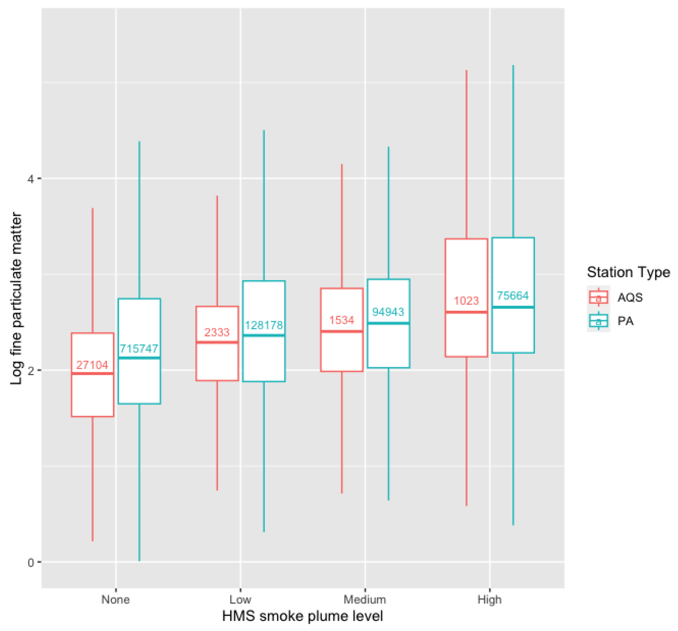
2.1.1. Satellite-Derived Smoke Plume Indicators

Exposure to wildland fire smoke is assessed using smoke plume indicators supplied by the HMS [33]. This automated data product integrates observations from multiple polar and geostationary satellites to generate polygons representing smoke plume extents on a daily basis. Distinct polygons are provided for low-, medium-, and high-density plumes. These smoke plume indicators tend to underestimate the actual intensity of smoke, as they primarily rely on satellite imagery with an approximate spatial resolution spanning several miles [34,35]. Additionally, smoke visibility is limited to daytime hours, resulting in a significant underestimation of smoke levels during the night. While the HMS data are among the most reliable widely-available measures of plume extent, Ref. [35] shows that it may underestimate wildland fire contribution to PM 2.5 .

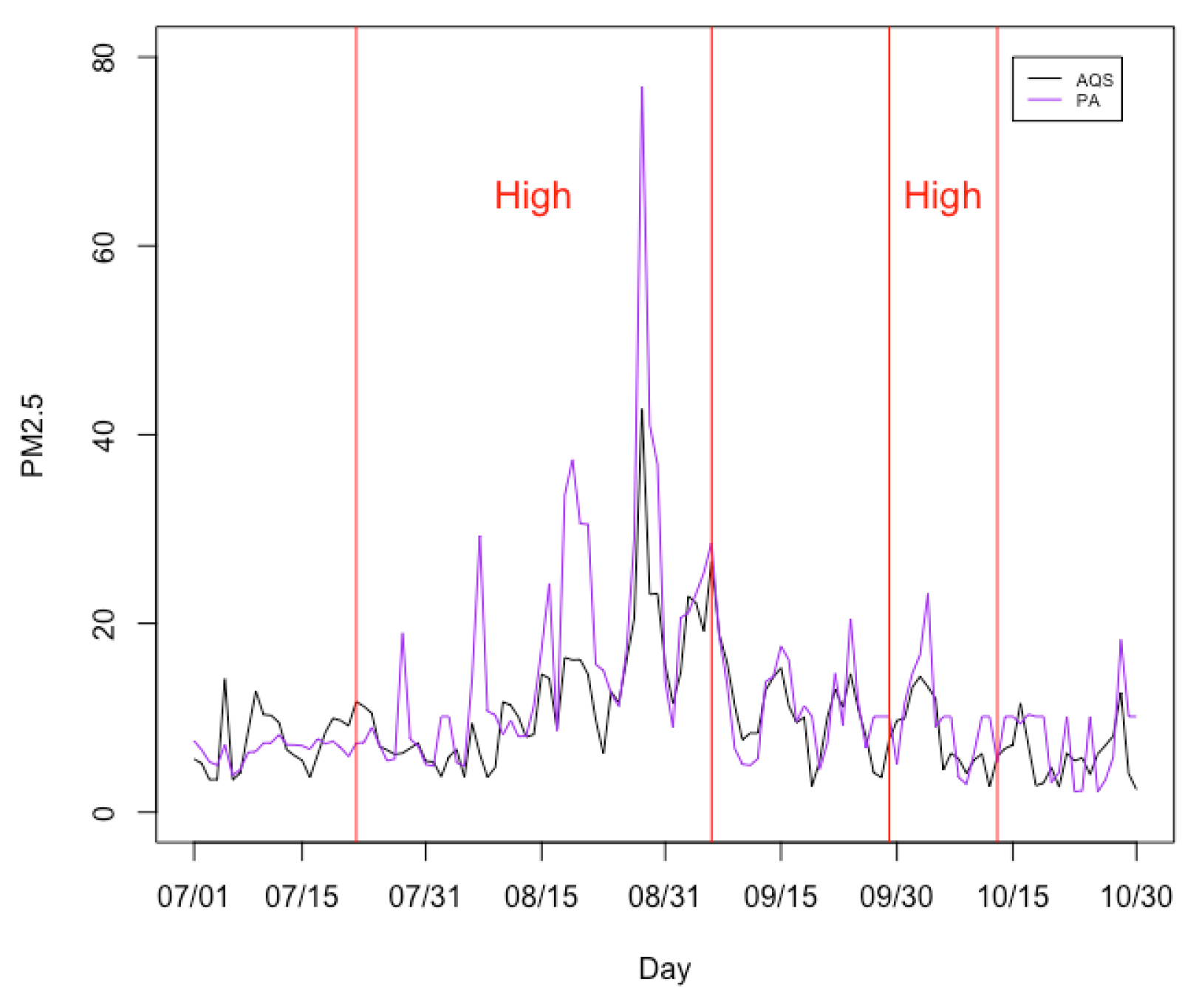
2.1.2. AQS Monitoring Stations

The AQS monitoring stations, deployed by the US Environmental Protection Agency (EPA) and state, local, and tribal air pollution control agencies, provide precise PM 2.5 measurements. However, their distribution is spatially sparse due to the high cost and complexity associated with their installation and maintenance.

2.1.3. PA Sensors

PA sensors are low-cost monitoring devices deployed by individuals and organizations for continuous ambient air pollutant tracking. Even during wildland fire events, PA sensors have been show to strongly correlate with gold standard measurements [36]. Despite their affordability and ease of installation, PA sensors offer less accurate PM 2.5 readings and are significantly influenced by environmental factors, such as temperature and humidity [15]. We use bias corrected data for all analyses. However, this initial bias correction based on Barkjohn et al. in [15] may be insufficient because it only depends on a linear trend in temperature and humidity and is constant across space and time. Therefore, our Bayesian data fusion model adds a more flexible spatiotemporal bias correction term.
Before fitting the statistical model, we implemented several pre-processing steps on the PA data and standardized temperature and humidity. PA stations feature two independent channels, Channel A and Channel B, both of which measure ambient PM 2.5 independently. To achieve a more accurate estimation of the actual ambient PM 2.5 concentration, we discarded readings where the measurement difference exceeded 200 μ g /m 3 . We discarded readings where the daily readings have constant high PM 2.5 readings over 2000 μ g /m 3 . We choose the threshold of value of 2000 μ g /m 3 because some PA stations have a constant reading around 2000 μ g /m 3 , and all other stations have values at most at 800 μ g /m 3 , which suggests a data collection error. Subsequently, the mean reading from Channel A and Channel B was considered as the PA measurement.
A majority of PA stations measure temperature (in Fahrenheit) and relative humidity. Because the temperature and humidity are spatially smooth, we employ a 10-nearest-neighbor approach to impute stations with missing temperature and humidity values and unobserved sites in California.
In 2021, more than 7800 outdoor PA sensors were operational in California. We only use outdoor sensor for comparison with AQS stations. We have included only those PA stations that reported fewer than 18 missing days during the fire seasons, resulting in a total of 1080 for 2020 and 712 PA stations for 2021. Figure 2 displays the distribution of PM 2.5 , aggregated across stations for 2021, by smoke plume intensity. A similar pattern is observed in both PA stations and AQS stations where PM 2.5 measurements escalate in the presence of a smoke plume.
Figure 3 shows one AQS and a nearby PA monitor daily readings over the fire season in 2021. For this stations, the two types of monitors have a high degree of correlation, and both monitors’ readings are elevated when under the high smoke plume. Figure 4 investigates the relationship between AQS stations and their corresponding nearby PA sites across California. For each AQS site, we compute its correlation with the closest PA site. Figure 4 plots these correlations, binned by the distance between the AQS and PA sites. The correlation is high when the stations are close and decreases with distance, suggesting that PA data will be a useful supplement to the spatial model.

2.2. Statistical Model

We propose a multi-resolution Bayesian model for modeling AQS and PA measurements jointly in the spectral domain. Let Y 1 t ( s ) and Y 2 t ( s ) be AQS and PA measurements, respectively, for spatial location s at time (day) t { 1 , , n t } , and X t ( s ) = { X 0 t ( s ) , , X p t ( s ) } be a corresponding vector of covariates with X 0 t ( s ) = 1 for the intercept. The p = 5 covariates are temperature, relative humidity and indicators of low, medium and high density smoke plumes at site s and day t. We note that temperature and relative humidity are standardized to have mean zero and variance one and that the AQS and PA measurements are not taken at the same spatial locations.
The observations are decomposed as Y j t ( s ) = Z j t ( s ) + ε j t ( s ) for j { 1 , 2 } , where j = 1 and j = 2 indicate AQS and PA monitors, respectively, Z 1 t ( s ) and Z 2 t ( s ) are spatiotemporal processes, and ε j t ( s ) i n d e p Normal ( 0 , τ j 2 ) is error. The time span of our data is relatively short, therefore, its reasonable to assume the spatiotemporal processes are stationary within the modeling period. We will apply Fourier transformation to the spatiotemporal processes Z j t ( s ) with respect to time to remove the temporal dependence. The resulting spectral processes Z j l * ( s ) capture periodicity, are independent over frequency { ω l , l = 1 , , n t } and spatially correlated. For time series observed at equal time intervals, we can apply the DFT. The spectral processes at frequency ω l is
Z j l * ( s ) = t = 1 n t exp ( i t ω l ) Z j t ( s )
and measures the variation in Z j t ( s ) at frequency ω l . Terms with small ω l (low frequency) represent long-term trends such as month-to-month averages and terms with large ω l (high frequency) represent short-term trends such as day-to-day variation. Let { Z j 1 * ( s ) , , Z j n t * ( s ) } be the unique real components of the DFT of { Z j 1 ( s ) , , Z j n t ( s ) } at frequencies { ω 1 , , ω n t } with ω 1 ω n t .
The spectral processes Z j l * ( s ) are dependent across j = 1 , 2 , as they represent the two networks measuring the same underlying PM 2.5 process. They are also spatially dependent processes as locations nearby may exhibit similar periodicity. We model the cross network dependence and spatial dependence for each ω l as
Z 1 l * ( s ) = U l ( s ) and Z 2 l * ( s ) = A l U l ( s ) + V l ( s ) ,
where spatial process U l ( s ) is the true PM 2.5 concentration for frequency l. The PA stations are assumed to be measuring a biased and noisy version of the true PM 2.5 with discrepancy V l ( s ) . The coefficient A l controls the dependence across networks. Both the bias V l ( s ) and cross-dependence A l vary by ω l to allow for a multi-resolution calibration of the two networks. We model A l linearly as A l = β A 0 + β A 1 · ω l , where β A 0 and β A 1 are unknown coefficients. This allows the correlation between the processes to vary stochastically with frequency. For example, if PA is more reliable for long-term trends than day-to-day variation, then we expect larger (smaller) correlation between networks for small (large) ω l .
The true process U l ( s ) and discrepancy term V l ( s ) are both regressed onto the covariates. Since we are developing a model in the spectral domain, we will also apply DFT to each covariate in X t ( s ) with respect to time and denote this as X j * ( s ) = { X 0 l * ( s ) , , X p l * ( s ) } Define the covariates for the true process U l as X u l * ( s ) = X j * ( s ) , containing all five covariates, and define X v l ( s ) = { X 0 l * ( s ) , X 1 l * ( s ) , X 2 l * ( s ) } to include only temperature and relative humidity for bias correction [15]. We model U l ( s ) and V l ( s ) as independent (with each other and over l) Gaussian processes with means E { U l ( s ) } = X u l * ( s ) β u and E { V l ( s ) } = X v l * ( s ) β v , variances Var { U l ( s ) } = σ u l 2 and Var { V l ( s ) } = σ v l 2 , and spatial correlations Cor { U l ( s ) , U l ( s ) } = exp ( | | s s | | / ρ u ) and Cor { V l ( s ) , V l ( s ) } = exp ( | | s s | | / ρ v ) .
The regression coefficients β u = ( β u 0 , , β u p ) T control the effects of the covariates on the true PM 2.5 process U. Although we specify the model in the spectral domain, the DFT is a linear operator and thus the covariates can be interpreted as usual in the spatial domain since the mean AQS response is
E { Y 1 t ( s ) } = X t ( s ) β u
Therefore, β u is of primary interest. In particular, the components of β u that correspond to the smoke plume indicators are used to summarize the wildland fire contribution to PM 2.5 .
The regression coefficients β v = ( β v 0 , β v 1 , β v 2 ) T control the effect of the covariates on the discrepancy term V, and thus the contribution of the covariates to the PA bias. By allowing the covariance parameters σ u l 2 and σ v l 2 to vary by frequency (l), we allow for a different degree of dependence between the networks at different temporal scales, with
Cor { Z 1 l * ( s ) , Z 2 l * ( s ) } = A l A l 2 + σ v l 2 / σ u l 2 .
The prior for the variance components is
σ u l 2 InvGamma ( a u l , b u l ) and σ v l 2 InvGamma ( a v l , b v l )
where the hyperparameters are modelled as log-linear in frequency, e.g., log ( a u l ) = γ a u 1 + γ a u 2 · ω l the prior captures the intuition that the variance is higher in month-to-month variation than day-to-day variation, and the correlation between two sources vary over frequencies.

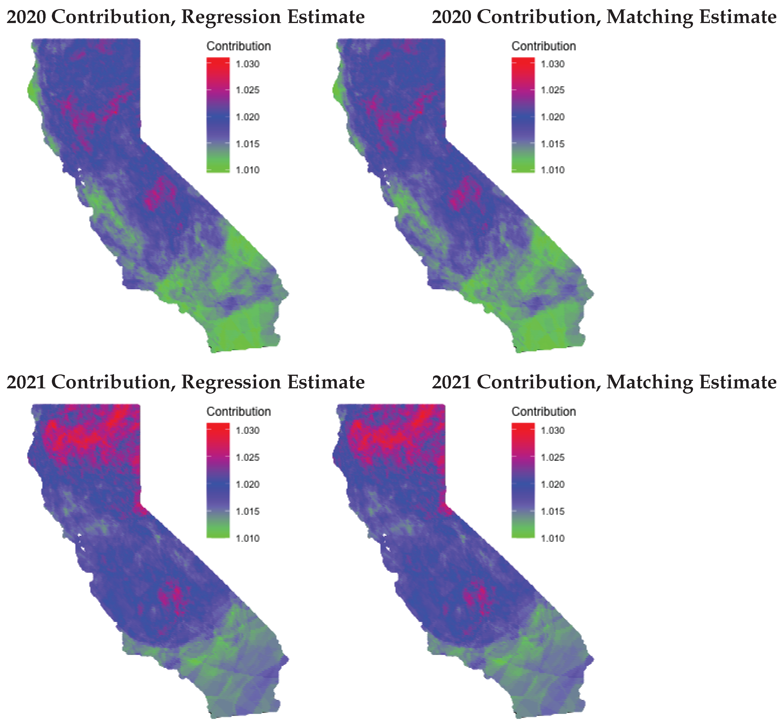
2.3. Quantifying the Wildland Fire Contribution

To estimate the PM 2.5 contribution from wildfire, given the estimated parameters above, we consider two metrics based on either regression or matching. For the regression metric, let X t 0 ( s ) be the covariate vector with three plume indicators fixed at zero. For the matching estimator, define P ( s ) as the set of days for which site s is in a smoke plume (any density) and P ¯ ( s ) as the set of non-plume days. We match each plume day with a non-plume day with similar meteorology and time period. Let A t ( s ) = P ¯ ( s ) { t 30 , , t + 30 } be the set of non-plume days within 30 days of plume day t. For each plume day, we selected the matching day m t ( s ) as
m t ( s ) = arg min d A t ( s ) | temp t ( s ) temp d ( s ) | + ϕ | humidity t ( s ) humidity d ( s ) |
where ϕ above is a scaling factor adjusting the magnitude of humidity and temperature, we set ϕ = 1 so that the best matching station has equal weights on temperature and humidity. Then at site s the estimated contribution from wildland fires per day are
  • Regression estimator: δ 1 ( s ) = 1 n t t = 1 n t { X t ( s ) X t 0 ( s ) } β u
  • Matching estimator: δ 2 ( s ) = 1 n t t P ( s ) { Z 1 t ( s ) Z 1 t ( s ) } for t = m t ( s ) .
In the matching estimator, Z 1 t ( s ) is the true PM 2.5 , the transformed pairs of Z 1 l * ( s ) in (2) obtained by inverse DFT, and thus this estimator accounts for spatiotemporal bias and correlation. Since the analysis is on the log-scale, we plot exp { δ 1 ( s ) } and exp { δ 2 ( s ) } which estimate the multiplicative effect, i.e., exp { δ 1 ( s ) } = 1.05 corresponds to a 5% increase in PM 2.5 in the presence of a smoke plume.

2.4. Computational Algorithm

To complete the Bayesian model, we specify uninformative prior distributions for the model parameters. The regression coefficients have Gaussian priors β u , β v Normal ( 0 , c 2 I p + 1 ) . The variance parameters have conjugate priors τ j 2 InvGamma ( a , b ) . The hyperpameters have Gaussian priors γ a u 1 , γ a u 2 , γ a v 1 , γ a v 2 Normal ( 0 , c 2 ) . To give uninformative priors we set a = b = 0.01 and c = 10 . Due to poor convergence, the dependence parameters β A 0 and β A 1 were fixed based on cross-validation to minimize mean squared prediction error for AQS stations.
The main computational bottleneck of spatial modeling is manipulating spatial covariance matrices to estimate the range parameters ρ u and ρ v . Given the large size of the air pollution dataset, a reasonable simplification is to estimate the range parameters using variogram and then assume they are fixed for the purpose of fitting the final model. The estimated spatial range from variograms are ρ u = 177 and ρ v = 111 kilometers.
Given the range parameters are fixed, the remaining parameters are estimated using Markov Chain Monte Carlo (MCMC) methods. In particular, we perform Gibbs sampling steps for most parameters and Metropolis sampling for some hyperparameters. We generate 8000 posterior samples and discard the first 5000 as burn-in. The MCMC details are relegated to the Appendix A, Appendix B and Appendix C. Appendix A gives the details of each MCMC step. A simulation study is included in the Appendix B to verify the algorithm produces reliable parameter estimates. Convergence is monitored using trace plots for several representative parameters shown in Appendix C.

3. Results

3.1. Summary of the Fitted Model

Table 1 gives the estimates of the regression coefficients for both the true process β u and bias correction term β v . All three smoke plume levels positively affect PM 2.5 concentrations, with high smoke plumes having the greatest impact, followed by medium and low smoke plumes. These results are consistent between 2020 and 2021. The bias correction terms, however, are not significant. Given that PA readings have already been corrected as per [15] using temperature and relative humidity, it is reasonable that these variable do not explain trends in bias. We note that our model does include more general spatiotemporal bias correction in V l ( s ) and including this bias term leads to improved results, as discussed below.
Figure 5 plots the estimated wildland fire contribution both years and both metrics. The estimated wildland fire contribution ranges from a 1–3% increase in PM 2.5 , depending on the location. Both metrics yield similar estimates of contribution and spatial patterns. The impact of wildfires varies across the state and years. In 2020, both Northern and Central California experienced significant wildfire impacts, while only Northern California faced major effects in 2021. This is in line with the fact that 2020 had the highest frequency of wildfires across all states, whereas 2021 witnessed a single, massive wildfire in Northern California [37]. Figure 6 shows the posterior standard deviation of the contribution. The uncertainty of estimation in 2020 is generally smaller than 2021. Moreover, both estimators give roughly the same undertainty estimation, with matching estimator only slightly more stable than regression estimate.
In addition to covariate effects, the data-fusion model provides an evaluation of the concordance between AQS and PA stations. Equation (4) defines the correlation between the two networks as a function of the spectral frequency, ω l . Figure 7 plots the correlation between AQS and PA by period, i.e., 1 / ω l . For example, period 7 (30) corresponds to variation that occurs on a weekly (monthly) scale. Figure 7 shows that the correlation between AQS and PA stations increases from short-term, such as day-to-day variation, to long-term, such as month-to-month variation. In the short-term, the correlation is lower since the readings are taken at different spatial locations and are subject to small scale variability. Over the long run, the correlation is higher as both sources estimate ambient unbiased PM 2.5 readings.

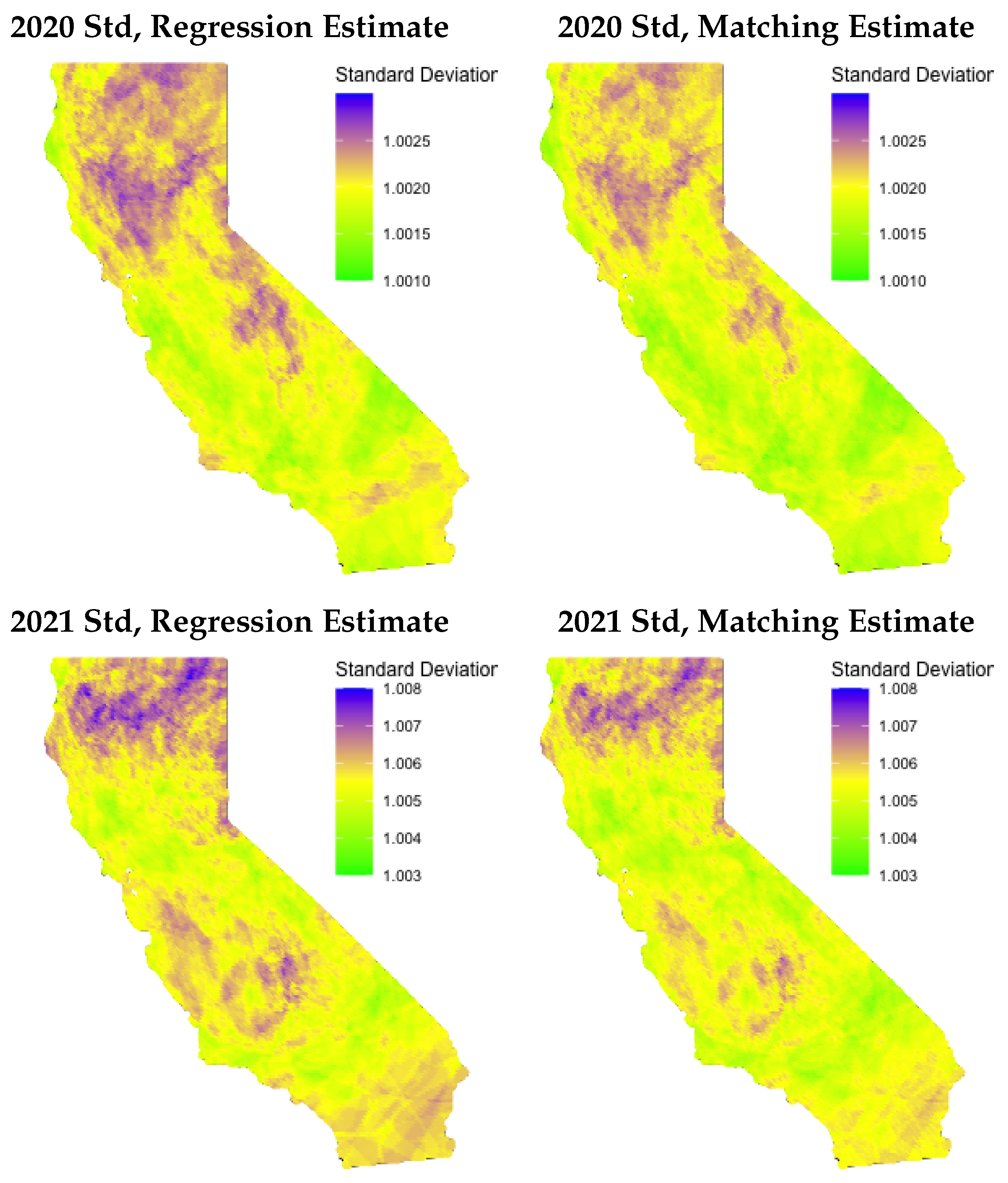
3.2. Model Comparisons

To assess the effectiveness of integrating additional PA readings, we compared the proposed data-fusion model (“Data fusion”) with two simpler alternatives. The first uses only AQS data (“AQS only”) and discards the PA data (i.e., sets A l = 0 for all l). The second naively (“Naive”) combines AQS and PA data and treats them as a single source without spatiotemporal bias adjustment (i.e., sets A l = 1 and V l ( s ) = 0 for all s , and includes an indicator variable in the regression term, β u , to distinguish two types of data).
The estimated parameters for each model, along with the corresponding posterior standard deviations, are presented in Table 2. Clearly, incorporating PA monitors significantly reduces the posterior standard deviation. For many of the parameters the reduction in uncertainty is striking, with the standard deviation being 2–4 times smaller for the data-fusion model. Also, with the AQS-only model, only high smoke plumes exhibit a significant contribution due to a higher standard deviation. In contrast, when merging AQS and PA data, both medium and high smoke plume levels show significant contributions.
Furthermore, to verify that our proposed methodologies not only improve parameter estimation but also lead to accurate PM 2.5 predictions, we performed a 5-fold cross-validation for the three models using data from 2021. We randomly split the AQS stations into five folds. For each fold, we build predictive models based on the other AQS stations and all PA stations and make predictions at the test sites. Performance was compared based on three key metrics: Root mean squared error, 95% prediction coverage, and prediction variance. For all models, we fix the spatial range parameters ( ρ u and ρ v ) based on the variogram analysis of the full dataset. The cross-dependence parameter A l is fixed at 0.2.
The results in Table 3 show that the performance of the AQS-only analysis is fairly similar to the proposed data-fusion approach, with slightly smaller prediction mean squared error and larger average prediction variance. Therefore, carefully including the additional PA data mainly reduces the prediction variance. However, naively including the PA data gives much higher prediction errors and low coverage.
In summary, the AQS-only and data fusion model produce fairly similar out-of-sample prediction accuracy, therefore the main benefit of including the PA data is reducing uncertainty in parameter estimates. Also, the Naive model gives a 50% larger RMSE and low coverage, emphasizing the need for a careful data fusion approach.

4. Discussion

In this study, we examine the impact of wildland fires on PM 2.5 concentrations in California during the fire seasons of 2020 and 2021. As we can see from Figure 5, PM 2.5 contributes to about a 3% increase in parts of California that are heavily affected by wildland fires in both 2020 and 2021; in most other areas the increase ranges from 1.0% to 2.3%. To obtain precise estimates, we combine remotely-sensed smoke-plume indicators with AQS and PA measurement networks. To model the spatiotemporal correlation of PM 2.5 concentration and relationship between AQS and PA monitors, we first transform the data from spatial domain to frequency domain, and then use a data-fusion approach to model spatial correlations while accounting for biases in the PA data. Furthermore, we use a Bayesian approach to compute posterior distributions of the quantities of interest to fully characterize uncertainty.
As shown in Table 2, we find that including PA monitors significantly increases the precision of the estimated contribution of wildland fire smoke to total PM 2.5 . Using only AQS data we find that medium and high smoke plume levels significantly contribute to PM 2.5 concentration with standard deviations as large as 0.017, and the data fusion approach that supplements AQS with PA data gives similar parameter estimation, with standard deviation as small as 0.004. Moreover, the data fusion model also estimates a significant low smoke plume level contribution. However, as we can see from Table 3, since PM 2.5 concentration is relatively smooth across space and AQS stations are evenly distributed across the state, incorporating PA readings does not improve prediction performance even for the data-fusion approach. Comparing prediction performance does reveal that simple data fusion model such as the model that ignores bias in the PA data gives inferior prediction results. Based on Table 1, with our model, all three smoke plume levels demonstrate a significant contribution to PM 2.5 concentration, and the impact varies across different regions depending on the year. This study highlights the value of utilizing both AQS and PA data in understanding the impact of wildfires on air quality and informs future monitoring and management efforts.
There are some limitations of our current work. First, as mentioned above, the satellite-derived smoke plume levels might underestimate the actual smoke level, which may lead to underestimation of wildfires’ contribution to PM 2.5 [34]. Second, due to computational limitations and poor MCMC convergence, we fixed the spatial correlation range parameters for both AQS and PA monitors and parameters that control the relationships between AQS and PA data. The analysis would more fully quantify uncertainty if we are able to implement a fully Bayesian analysis. Our analysis of the smoke contribution is also limited because we only consider temperature and relative humidity and no other meteorological variables or anthropogenic sources. Another limitation is that we use only HMS smoke indicators to denote fire smoke, which has known limitations [35]. Although we estimate the relationship between HMS and PM2.5 concentration using the data, HMS may fail to capture the smoke contribution from some fires.
We have taken a purely statistical approach to estimating the contribution of wildland fires on ambient air pollution. An area of future work is to incorporate numerical models to simulate the process. Dispersion models, e.g., HySPLIT [38], combine the location and size of fires and meteorological conditions in a mathematical model to track particulate matter emanating from a fire. Of course, numerical models also have bias and other limitations [39], but combining their output within our statistical framework would likely further refine our estimates. Further, instead of using one range parameter for all frequencies, it is possible to get variogram estimates of ranges over frequencies. Similarly, instead of assuming the same β u and β v for all locations, it may be better to estimate spatially-varying β u and β v , although this would be computationally intensive. To extend the current work, we can estimate the contribution over the entire U.S., although more efficient computational methods would be required for this analysis.

Author Contributions

Conceptualization, A.G.R. and B.J.R.; methodology, H.Y., Y.G., B.J.R.; validation, H.Y., S.R.-S.; formal analysis, H.Y.; data curation, H.Y., S.R.-S.; writing-original draft preparation, H.Y.; writing—review and editing, S.R.-S., B.J.R., Y.G., A.G.R. All authors have read and agreed to the published version of the manuscript.

Funding

This research was funded by the National Institutes of Health (R01ES031651-01) and the National Science Foundation (DMS2152887).

Data Availability Statement

AQS data is a publicly available dataset, which is part of this study. This data can be found on EPA website https://aqs.epa.gov/aqsweb/airdata/download_files.html (accessed on 1 April 2023). PA data is a 3rd party data and restrictions apply to the availability of these data. Data was obtained from Purple Air and are available from PurpleAir API https://community.purpleair.com/t/making-api-calls-with-the-purpleair-api/180 (accessed on 1 April 2023) with the permission of Purple Air. HMS smoke plume data is publicly available and can be downloaded at Office of Satellite and Product Operations website https://www.ospo.noaa.gov (accessed on 1 April 2023). The codes to download and analyze data in this paper is available at this GitHub repo https://github.com/hyang199723/PAFusion (uploaded on 30 June 2023).

Acknowledgments

This work does not represent EPA views.

Conflicts of Interest

The authors declare no conflict of interest.

Appendix A. MCMC Algorithm

Assume the n 1 AQS monitors are at spatial locations s 1 , , s n 1 and the n 2 PA monitors are located at s n 1 + 1 , , s n s for n s = n 1 + n 2 . The observations can be written as the vectors Y 1 t = [ Y 1 t ( s 1 ) , , Y 1 t ( s n 1 ) ] T , Y 2 t = [ Y 2 t ( s n 1 + 1 ) , , Y 1 t ( s n s ) ] T and Y t = ( Y 1 t T , Y 2 t T ) T . Similarly, for frequency l let Y j l * , U j l and V j l be vectors of length n j and Y l * , U l and V l be vectors of length n s , analogous to Y t . The covariate matrices of size n j × p are denoted X j l * and X l * is the n s × p matrix that stacks X 1 l * and X 2 l * . Then the model in the spectral domain is
Y 1 l * = U l + E 1 l and Y 2 l * = A l U l + V 2 l + E 2 l
where E j l i n d e p Normal ( 0 , τ j 2 I n j ) . Using this notation, the spatial models are defined by E ( U j l ) = X j l * β u , E ( V j l ) = X j l * β v , Cov ( U j l , U k l ) = σ u l 2 Σ u j k and Cov ( V j l , V k l ) = σ v l 2 Σ v j k . The full n s × n s spatial correlation matrices are denoted Σ u and Σ v .
Each MCMC iteration we impute missing data and update the error variance parameters in the spatial domain, and then update all remaining parameters in the spectral domain. The missing values are simply drawn from the univariate normal distribution
Y j t | rest Normal ( Z j t ( s ) , τ j 2 )
independently over j and t. The error variances are drawn from full conditional distribution τ 1 2 | rest InvGamma [ n 1 n t / 2 + a , i = 1 n 1 t = 1 n t { ( Y 1 t ( s i ) Z 2 t ( s i ) } 2 / 2 + b ] and τ 2 2 | rest InvGamma [ n 2 n t / 2 + a , i = n 1 + 1 n s t = 1 n t { ( Y 2 t ( s i ) Z 2 t ( s i ) } 2 / 2 + b ] .
After imputation in the spatial domain, the data are complete and can be projected into the spectral domain where they are independent over time. The spatial processes are updated as
U l | rest Normal Ω u l T A l 1 ( Y l * V l ) + 1 σ u l 2 Σ u 1 X l * β u , Ω u l V 2 l | rest Normal Ω v l 1 τ 2 2 ( Y 2 l * A l U 2 l ) + 1 σ v l 2 Σ v 22 1 X 2 l * β v , Ω v l
where A l k is diagonal with first n 1 elements equal one and the remaining n 2 elements equal A l k , T is diagonal with first n 1 elements equal τ 1 2 and the remaining n 2 elements equal τ 2 2 , V l is the vector with n 1 zeros followed by V 2 l , Ω u l 1 = T A l 2 + 1 σ u l 2 Σ u 1 and Ω v l 1 = 1 τ 2 2 I n 2 + 1 σ v l 2 Σ v 22 1 .
The regression coefficients and bias parameters are updated as
β u | rest Normal P u l = 1 n t 1 σ u l 2 X l * T Σ u 1 U l , P u β v | rest Normal P v l = 1 n t 1 σ v l 2 X 2 l * T Σ v 22 1 V 2 l , P v
where P u 1 = l = 1 n t 1 σ u l 2 X l * T Σ u 1 X l * + 1 c 2 I p and P v 1 = l = 1 n t 1 σ v l 2 X 2 l * T Σ v 22 1 X 2 l * + 1 c 2 I p . The remaining hyperparameters are updated as
σ u l 2 | rest InvGamma n s 2 + a u l , ( U l X l * β u ) T Σ u 1 ( U l X l * β u ) 2 + b u l σ v l 2 | rest InvGamma n 2 2 + a v l , ( V 2 l X 2 l * β v ) T Σ v 22 1 ( V 2 l X 2 l * β v ) 2 + b v l .
Finally, γ a u 1 , γ a u 2 , γ a v 1 and γ a v 2 are updated using a Metropolis step with Gaussian candidate distribution tuned to give acceptance rate around 0.4.

Appendix B. Simulation Results

We conduct a simulation study to demonstrate the reliability of the MCMC algorithm. The regression parameters, β u and β v , are fixed at the mean of the 2021 model output in Table 1. We generate a total number of 80 AQS stations and 500 PA stations with 60 time steps. The spatial locations are randomly sampled from the region ( 0 , 15 ) 2 . The data was generated in the frequency domain using the following equations:
Y 1 l ( s ) = U l ( s ) + ϵ 1 ( s ) and Y 2 l ( s ) = A l U l ( s ) + V 2 l ( s ) + ϵ 2 ( s ) .
The variables U l and V l are drawn from Gaussian processes as described in (2). The range parameters are set to ρ u = 2 and ρ v = 4 . The error variances of ϵ 1 ( s ) and ϵ 2 ( s ) are set to 1.6 and 3.6, respectively. The values of A l are fixed at the best A l selected from the real data which is A l = 0.2 .
To simulate realistic smoke plume frequencies, we assigned percentages to represent the occurrence of low, medium, and high smoke plume levels. Specifically, 20% of the days corresponded to low smoke plume levels, 15% to medium levels, and 10% to high levels. Temperature and humidity values were randomly generated from standard normal distributions.
The covariates were initially generated in the time domain and then transformed to the frequency domain. The values of σ u l form a decreasing sequence ranging from 50 to 10, with larger values assigned to lower frequencies. Similarly, σ v l follows a decreasing sequence from 40 to 10. Finally, the values of β u and β v are the mean values from Table 1.
We generate 50 datasets from this model. For each simulated dataset, we fit the model with ρ u , ρ v and A l fixed at the true values and generate 8000 MCMC iterations and discard the first 5000 as burn-in. Since our main interest is in the covariate effects, for each dataset we record the effective sample size of the MCMC algorithm [40] and the posterior mean estimator and 95% posterior interval.
For each dataset and each parameter, we compute the posterior mean, standard deviation and 95% interval and measure MCMC convergence using the effective sample size. The average of the posterior means, standard deviations and effective samples sizes, and the empirical coverage of 95% intervals are shown in Table A1. The posterior means show small bias, the coverage is near the nominal level and the effective sample size coefficients indicate reasonable convergence.
Table A1. True value used for the fixed effects for the true PM 2.5 ( β u ) and bias ( β v ) to simulate data and the average (SD) over the 50 datasets of the posterior mean estimators (“Ave post mean”), coverage of 95% posterior intervals and average (SD) effective sample size based on 3000 MCMC iterations.
TypeCovariateTrue ValueAverage Post MeanCoverageESS
PM 2.5 Temperature0.1180.117 (0.013)100%420.23 (0.14)
Humidity0.0640.069 (0.022)96%307.27 (0.10)
Plume-Low0.0070.006 (0.132)100%875.99 (0.29)
Plume-Medium0.0220.020 (0.037)98%376.91 (0.13)
Plume-High0.0490.050 (0.176)100%480.22 (0.16)
BiasTemperature−0.0020.003 (0.019)92%168.75 (0.06)
Humidity0.0120.009 (0.041)96%176.97 (0.06)

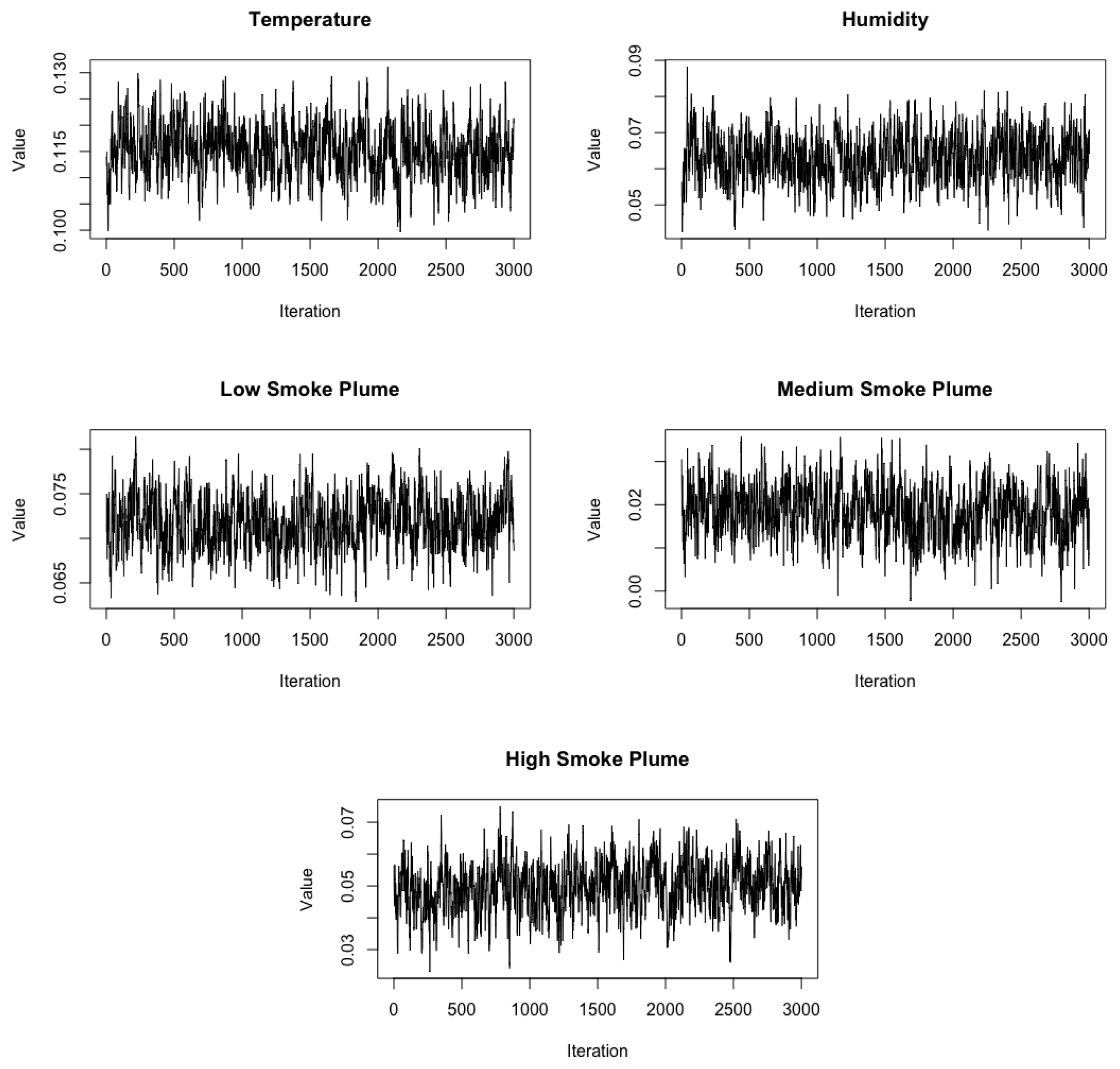
Appendix C. MCMC Convergence

We display several representative trace plots of the data fusion model to verify the convergence of our MCMC algorithm for the 2021 CA analysis. After burn-in, the MCMC chains appear to have converged.
Figure A1. Trace plots of parameters of interest ( β u ) for the 2021 California data analysis.
Remotesensing 15 04246 g0a1

References

  1. Dennekamp, M.; Abramson, M.J. The effects of bushfire smoke on respiratory health. Respirology 2011, 16, 198–209. [Google Scholar] [CrossRef]
  2. Dennekamp, M.; Straney, L.D.; Erbas, B.; Abramson, M.J.; Keywood, M.; Smith, K.; Sim, M.R.; Glass, D.C.; Del Monaco, A.; Haikerwal, A.; et al. Forest fire smoke exposures and out-of-hospital cardiac arrests in Melbourne, Australia: A case-crossover study. Environ. Health Perspect. 2015, 123, 959–964. [Google Scholar] [CrossRef] [PubMed]
  3. Melnick, R.S. Regulation and the Courts: The Case of the Clean Air Act; Brookings Institution Press: Washington, DC, USA, 2010. [Google Scholar]
  4. Sager, L.; Singer, G. Clean Identification? The Effects of the Clean Air Act on Air Pollution, Exposure Disparities and House Prices. 2022. Available online: https://www.lse.ac.uk/granthaminstitute/wp-content/uploads/2022/05/working-paper-376-Sager-Singer_May-2023.pdf (accessed on 1 May 2023).
  5. McClure, C.D.; Jaffe, D.A. US particulate matter air quality improves except in wildfire-prone areas. Proc. Natl. Acad. Sci. USA 2018, 115, 7901–7906. [Google Scholar] [CrossRef] [PubMed]
  6. Johnston, F.H.; Henderson, S.B.; Chen, Y.; Randerson, J.T.; Marlier, M.; DeFries, R.S.; Kinney, P.; Bowman, D.M.; Brauer, M. Estimated global mortality attributable to smoke from landscape fires. Environ. Health Perspect. 2012, 120, 695–701. [Google Scholar] [CrossRef] [PubMed]
  7. Rappold, A.G.; Stone, S.L.; Cascio, W.E.; Neas, L.M.; Kilaru, V.J.; Carraway, M.S.; Szykman, J.J.; Ising, A.; Cleve, W.E.; Meredith, J.T.; et al. Peat bog wildfire smoke exposure in rural North Carolina is associated with cardiopulmonary emergency department visits assessed through syndromic surveillance. Environ. Health Perspect. 2011, 119, 1415–1420. [Google Scholar] [CrossRef] [PubMed]
  8. Haikerwal, A.; Akram, M.; Sim, M.R.; Meyer, M.; Abramson, M.J.; Dennekamp, M. Fine particulate matter (PM2.5) exposure during a prolonged wildfire period and emergency department visits for asthma. Respirology 2016, 21, 88–94. [Google Scholar] [CrossRef]
  9. Thilakaratne, R.; Hoshiko, S.; Rosenberg, A.; Hayashi, T.; Buckman, J.R.; Rappold, A.G. Wildfires and the changing landscape of air pollution–related gealth burden in California. Am. J. Respir. Crit. Care Med. 2023, 207, 887–898. [Google Scholar] [CrossRef]
  10. Li, L.; Girguis, M.; Lurmann, F.; Pavlovic, N.; McClure, C.; Franklin, M.; Wu, J.; Oman, L.; Breton, C.; Gilliland, F. Ensemble-based deep learning for estimating PM2.5 over California with multisource big data including wildfire smoke. Environ. Int. 2020, 145, 106143. [Google Scholar] [CrossRef]
  11. Romanov, A.A.; Tamarovskaya A., N.; Gusev B., A.; Leonenko, E.V.; Vasiliev, A.S.; Krikunov, E.E. Catastrophic PM2.5 emissions from Siberian forest fires: Impacting factors analysis. Environ. Pollut. 2022, 306, 119324. [Google Scholar] [CrossRef]
  12. Ikeda, K.; Tanimoto, H. Exceedances of air quality standard level of PM2.5 in Japan caused by Siberian wildfires. Environ. Res. Lett. 2015, 10, 105001. [Google Scholar]
  13. Larsen, A.E.; Reich, B.J.; Ruminski, M.; Rappold, A.G. Impacts of fire smoke plumes on regional air quality, 2006–2013. J. Expo. Sci. Environ. Epidemiol. 2018, 28, 319–327. [Google Scholar] [CrossRef] [PubMed]
  14. Matz, C.J.; Egyed, M.; Xi, G.; Racine, J.; Pavlovic, R.; Rittmaster, R.; Henderson, S.B.; Stieb, D.M. Health impact analysis of PM2.5 from wildfire smoke in Canada (2013–2015, 2017–2018). Sci. Total Environ. 2020, 725, 138506. [Google Scholar] [PubMed]
  15. Barkjohn, K.; Gantt, B.; Clements, A. Development and Application of a United States wide correction for PM2.5 data collected with the PurpleAir sensor. Atmos. Meas. Tech. Discuss. 2020, 2020, 7304881. [Google Scholar] [CrossRef]
  16. Tryner, J.; L’Orange, C.; Mehaffy, J.; Miller-Lionberg, D.; Hofstetter, J.C.; Wilson, A.; Volckens, J. Laboratory evaluation of low-cost PurpleAir PM monitors and in-field correction using co-located portable filter samplers. Atmos. Environ. 2020, 220, 117067. [Google Scholar] [CrossRef]
  17. Wallace, L.; Bi, J.; Ott, W.R.; Sarnat, J.; Liu, Y. Calibration of low-cost PurpleAir outdoor monitors using an improved method of calculating PM2.5. Atmos. Environ. 2021, 256, 118432. [Google Scholar] [CrossRef]
  18. Holder, A.L.; Mebust, A.K.; Maghran, L.A.; McGown, M.R.; Stewart, K.E.; Vallano, D.M.; Elleman, R.A.; Baker, K.R. Field evaluation of low-cost particulate matter sensors for measuring wildfire smoke. Sensors 2020, 20, 4796. [Google Scholar] [CrossRef]
  19. Kosmopoulos, G.; Salamalikis, V.; Pandis, S.; Yannopoulos, P.; Bloutsos, A.; Kazantzidis, A. Low-cost sensors for measuring airborne particulate matter: Field evaluation and calibration at a South-Eastern European site. Sci. Total Environ. 2020, 748, 141396. [Google Scholar] [CrossRef]
  20. Durrant-Whyte, H.; Henderson, T.C. Multisensor data fusion. In Springer Handbook of Robotics; Springer: Berlin/Heidelberg, Germany, 2016; pp. 867–896. [Google Scholar]
  21. Luo, R.C.; Kay, M.G. A tutorial on multisensor integration and fusion. In Proceedings of the IECON’90: 16th Annual Conference of IEEE Industrial Electronics Society, Pacific Grove, CA, USA, 27–30 November 1990; pp. 707–722. [Google Scholar]
  22. Reich, B.J.; Chang, H.H.; Foley, K.M. A spectral method for spatial downscaling. Biometrics 2014, 70, 932–942. [Google Scholar] [CrossRef]
  23. Warren, J.L.; Miranda, M.L.; Tootoo, J.L.; Osgood, C.E.; Bell, M.L. Spatial distributed lag data fusion for estimating ambient air pollution. Ann. Appl. Stat. 2021, 15, 323. [Google Scholar] [CrossRef]
  24. Friberg, M.D.; Zhai, X.; Holmes, H.A.; Chang, H.H.; Strickland, M.J.; Sarnat, S.E.; Tolbert, P.E.; Russell, A.G.; Mulholland, J.A. Method for fusing observational data and chemical transport model simulations to estimate spatiotemporally resolved ambient air pollution. Environ. Sci. Technol. 2016, 50, 3695–3705. [Google Scholar] [CrossRef]
  25. Friberg, M.D.; Kahn, R.A.; Holmes, H.A.; Chang, H.H.; Sarnat, S.E.; Tolbert, P.E.; Russell, A.G.; Mulholland, J.A. Daily ambient air pollution metrics for five cities: Evaluation of data-fusion-based estimates and uncertainties. Atmos. Environ. 2017, 158, 36–50. [Google Scholar] [CrossRef]
  26. Nguyen, H.; Cressie, N.; Braverman, A. Spatial statistical data fusion for remote sensing applications. J. Am. Stat. Assoc. 2012, 107, 1004–1018. [Google Scholar] [CrossRef]
  27. Gressent, A.; Malherbe, L.; Colette, A.; Rollin, H.; Scimia, R. Data fusion for air quality mapping using low-cost sensor observations: Feasibility and added-value. Environ. Int. 2020, 143, 105965. [Google Scholar] [CrossRef] [PubMed]
  28. Datta, A.; Saha, A.; Zamora, M.L.; Buehler, C.; Hao, L.; Xiong, F.; Gentner, D.R.; Koehler, K. Statistical field calibration of a low-cost PM2.5 monitoring network in Baltimore. Atmos. Environ. 2020, 242, 117761. [Google Scholar] [CrossRef] [PubMed]
  29. Lin, Y.C.; Chi, W.J.; Lin, Y.Q. The improvement of spatial-temporal resolution of PM2. 5 estimation based on micro-air quality sensors by using data fusion technique. Environ. Int. 2020, 134, 105305. [Google Scholar] [CrossRef]
  30. Gao, F.; Masek, J.; Schwaller, M.; Hall, F. On the blending of the Landsat and MODIS surface reflectance: Predicting daily Landsat surface reflectance. IEEE Trans. Geosci. Remote. Sens. 2006, 44, 2207–2218. [Google Scholar]
  31. Hu, D.g.; Shu, H. Spatiotemporal interpolation of precipitation across Xinjiang, China using space-time CoKriging. J. Cent. South Univ. 2019, 26, 684–694. [Google Scholar] [CrossRef]
  32. Stein, M.L. Statistical methods for regular monitoring data. J. R. Stat. Soc. Ser. Stat. Methodol. 2005, 67, 667–687. [Google Scholar] [CrossRef]
  33. National Oceanic and Atmospheric Administration. Hazard Mapping System Fire and Smoke Product. Available online: https://www.ospo.noaa.gov/Products/land/hms.html (accessed on 15 October 2022).
  34. O’Dell, K.; Ford, B.; Fischer, E.V.; Pierce, J.R. Contribution of wildland-fire smoke to US PM2.5 and its influence on recent trends. Environ. Sci. Technol. 2019, 53, 1797–1804. [Google Scholar] [CrossRef]
  35. Buysse, C.E.; Kaulfus, A.; Nair, U.; Jaffe, N.A. Relationships between particulate matter, ozone, and nitrogen oxides during urban smoke events in the western US. Environ. Sci. Technol. 2019, 53, 12519–12528. [Google Scholar] [CrossRef]
  36. Barkjohn, K.K.; Holder, A.L.; Frederick, S.G.; Clements, A.L. Relationships between particulate matter, ozone, and nitrogen oxides during urban smoke events in the western US. Sensors 2022, 22, 9669. [Google Scholar] [PubMed]
  37. California Department of Forestry and Fire Protection. Top 20 Largest California Wildfires. Available online: https://www.fire.ca.gov/our-impact/statistics (accessed on 1 February 2023).
  38. Draxler, R.; Rolph, G. HYSPLIT (HYbrid Single-Particle Lagrangian Integrated Trajectory) Model Access via NOAA ARL READY; NOAA Air Resources Laboratory: Silver Spring, MD, USA, 2010; Volume 25. Available online: https://www.ready.noaa.gov/HYSPLIT.php (accessed on 1 May 2023).
  39. Su, L.; Yuan, Z.; Fung, J.C.; Lau, A.K. A comparison of HYSPLIT backward trajectories generated from two GDAS datasets. Sci. Total Environ. 2015, 506, 527–537. [Google Scholar] [CrossRef] [PubMed]
  40. Geyer, C.J. Introduction to Markov Chain Monte Carlo. In Handbook of Markov Chain Monte Carlo; Chapman and Hall/CRC: Boca Raton, FL, USA, 2011; Volume 20116022, p. 45. [Google Scholar]
Figure 1. HMS smoke plume density (shaded regions) in California on 20 September 2021 and the locations of PA (purple dots) and AQS (black dots) monitoring stations.
Remotesensing 15 04246 g001
Figure 2. Distribution of log PM 2.5 ( μ g /m 3 ) by smoke plume level for PA and AQS stations. Four smoke plume levels from left to right are: no smoke, low, medium, and high plume density. The number of observations for each smoke plume level and each sensor type is displayed in the box.
Remotesensing 15 04246 g002
Figure 3. One AQS monitor at 37 20 N , 121 53 W (downtown San Jose) and a nearby PA monitor PM 2.5 readings over the fire season in 2021. Dates from 07/18 to 09/03 and 09/29 to 10/13 are covered in high smoke plume region and are indicated by “High” above.
Remotesensing 15 04246 g003
Figure 4. Sample correlation between AQS and nearby PA stations versus the distance (km).
Remotesensing 15 04246 g004
Figure 5. Smoke contribution to PM 2.5 . Contributions are exponentiated to reflect actual percentage contribution. For example, 1.01 and 1.03 mean wildfire contributes to roughly a 1% to 3% increase in PM 2.5 .
Remotesensing 15 04246 g005
Figure 6. Posterior standard deviation of smoke contribution to PM 2.5 . The posterior standard deviations are not exponentiated, and they show uncertainty estimation on the original scale.
Remotesensing 15 04246 g006
Figure 7. Posterior distribution of the correlation between AQS and PA by period. Small periods capture short-term variation, such as day-to-day variation, while large periods capture long-term variation, such as monthly trends.
Remotesensing 15 04246 g007
Table 1. Posterior mean (95% interval) for the model parameters. The regression coefficients are given separately for the true PM 2.5 process ( β u ) and bias correction ( β v ). A “***” indicates that the 95% interval excludes zero.
2020 Fire Season
ParameterTrue PM 2.5 Bias Correction
Temperature0.115 (0.106,0.125) ***−0.002 (−0.009,0.005)
Humidity0.064 (0.048,0.080) ***0.012 (−0.002,0.035)
Plume—Low0.007 (0.003,0.011) ***/
Plume—Medium0.022 (0.012,0.032) ***/
Plume—High0.049 (0.033,0.065) ***/
2021 Fire Season
ParameterTrue PM 2.5 Bias Correction
Temperature0.006 (0.004,0.008) ***0.006 (−0.003,0.015)
Humidity0.000 (−0.001,0.001)−0.011 (−0.026,0.003)
Plume—Low0.011 (0.001,0.021) ***/
Plume—Medium0.018 (0.007,0.029) ***/
Plume—High0.041 (0.031,0.051) ***/
Table 2. Posterior mean (standard deviation) for the model parameters β u for the CA data using the proposed data-fusion model, the model that uses only AQS data, and the naive data-fusion model that ignores bias in the PA data. A “***” indicates that the 95% interval excludes zero.
2020 Fire Season
ParameterData FusionAQS OnlyNaive
Temperature0.115 (0.005) ***0.105 (0.024) ***−0.418 (0.066) ***
Humidity0.064 (0.008) ***0.086 (0.022) ***−1.125 (0.052) ***
Plume—Low0.007 (0.002) ***0.005 (0.012)0.107 (0.078)
Plume—Medium0.022 (0.005) ***0.020 (0.014)0.271 (0.052) ***
Plume—High0.049 (0.008) ***0.042 (0.016) ***0.637 (0.079) ***
2021 Fire Season
ParameterData FusionAQS OnlyNaive
Temperature0.006 (0.001) ***0.015 (0.003) ***−0.014 (0.006) ***
Humidity0.000 (0.000)0.008 (0.002) ***−0.039 (0.003) ***
Plume—Low0.011 (0.004) ***−0.001 (0.014)−0.330 (0.032) ***
Plume—Medium0.018 (0.004) ***0.023 (0.016)0.230 (0.074) ***
Plume—High0.041 (0.005) ***0.054 (0.017) ***0.980 (0.071) ***
Table 3. Root mean squared error (“RMSE”), coverage of 95% prediction intervals (“Coverage”) and average prediction variance (“Ave Var”) for the cross-validation study comparing the proposed data fusion model to models that ignore PA data (“AQS only”) and includes PA data without bias correction (“Naive”).
ModelRMSECoverageAve Var
Data Fusion0.420.890.13
AQS only0.400.910.16
Naive0.660.730.18
Disclaimer/Publisher’s Note: The statements, opinions and data contained in all publications are solely those of the individual author(s) and contributor(s) and not of MDPI and/or the editor(s). MDPI and/or the editor(s) disclaim responsibility for any injury to people or property resulting from any ideas, methods, instructions or products referred to in the content.

