
Factors of Subsidence in Katy, Texas, USA

Department of Earth and Atmospheric Sciences, University of Houston, Houston, TX 77204, USA
*
Author to whom correspondence should be addressed.
Remote Sens. 2023, 15(18), 4424; https://0-doi-org.brum.beds.ac.uk/10.3390/rs15184424
Submission received: 10 August 2023
/
Revised: 2 September 2023
/
Accepted: 6 September 2023
/
Published: 8 September 2023
(This article belongs to the Special Issue Application of Satellite Remote Sensing in Solving Urban Geo-Environmental Issues II)
Abstract
:Coastal communities are susceptible to the damaging effects of land subsidence caused by both natural and anthropogenic processes. The Greater Houston area, situated along the Gulf Coast of Texas, has experienced some of the highest rates of subsidence in the United States. Previous work has extensively analyzed the role of groundwater levels and oil and gas extraction in land subsidence of the Greater Houston area, but has failed to adequately incorporate other significant contributing factors. In this research, we aim to fill that information gap by analyzing the individual effects of subsidence from multiple different processes including groundwater and hydrocarbon extraction rates with the addition of population growth, total annual precipitation, and total developed area in terms of impervious surfaces. We perform a full resolution InSAR analysis of the Katy area using Sentinel-1 data from 2017 to 2022 and compare contributors of subsidence to vertical displacement rates calculated by GNSS stations through a generalized linear regression analysis. The InSAR results show up to 1.4 cm/yr of subsidence in multiple areas of Katy, and the generalized linear regression results suggest that population growth and total developed area are two of the highest contributors to subsidence in the area.
1. Introduction
Land subsidence is a globally ubiquitous problem for coastal communities, including the Greater Houston area in Texas (Figure 1). Subsidence in the Greater Houston area is caused by a combination of natural and anthropogenic factors. Natural processes include sediment compaction, faulting, and salt migration [1,2]. These processes cause deformation over time at a steady rate due to their interaction with natural processes that offset subsidence, such as sedimentation and production of new soil through organic decay [3]. The main anthropogenic processes that are known to cause subsidence include groundwater withdrawal, oil and gas extraction [1,4], mining activity [5,6,7], and triggered geological processes such as reactivation of dormant faults [8]. As a result, the Greater Houston area has experienced some of the highest rates of subsidence in the United States, with up to 7 cm/yr in the downtown area from 1996–2003 [9] and up to 2 cm/year in the western suburbs of the city in more recent years [2,10]. This has led to significant challenges for the region, including increased flood risk, land loss, and infrastructure damage [11,12,13].
Previous works have focused extensively on the role of groundwater extraction and regional groundwater levels in subsidence of the Houston area [14,15,16,17,18]. There has also been analysis of land subsidence correlating with the extensive flooding caused by Hurricane Harvey in 2017 [19] as well as subsidence risk associated with aquifer storage and recovery [20]. The role of groundwater in land subsidence of the Greater Houston area has been thoroughly studied and established over the years. The relationship between subsidence and reactivation of faults and induced fault motion has also been established in multiple studies [2,21,22,23,24].
We present the first detailed study focusing on factors of subsidence specifically in the Katy area, a western suburb of Houston where the highest subsidence rate for the region is currently observed. Furthermore, we determine the most influential of the many factors of subsidence, and present a map of areas that are the most susceptible to infrastructure damage.
Recent studies [2,10,25] highlight that the maximum subsidence centers that were located in Spring and the Woodlands have transferred to the Katy area in the west. As such, we focus our analysis on the city of Katy due to the high deformation rate.
We use interferometric synthetic aperture radar (InSAR) to determine the rates and distribution of subsidence in the Katy area. We also combine a variety of datasets such as groundwater pumping rates, population growth, and global navigation satellite systems (GNSS) data to create a generalized linear regression model and determine the influence of various processes on subsidence.
2. Geological Background
Natural processes of subsidence such as faulting and sediment compaction are directly controlled by the underlying geology of the Greater Houston area. About 200 million years ago, the supercontinent Pangea was fractured and split into two new supercontinents, Laurasia and Gondwana. A section of the fracture expanded in Laurasia and created a large depression that became the Gulf of Mexico basin [26]. As new oceanic crust stretched and deepened the Gulf of Mexico basin in the middle Jurassic, between 160 and 140 million years ago, it was intermittently filled with seawater, which led to deposition of a salt unit up to 4 km in thickness [27,28]. These salt deposits were then overlain by an influx of terrigenous sediments carried to the gulf by large rivers such as the Mississippi [29]. Uplift of the Rocky Mountains to the west during the Laramide orogeny, during the Cretaceous about 70 million years ago, greatly increased the volume of sediment transported to the Gulf of Mexico. As a result of these processes, the Greater Houston area is underlain by a series of growth faults that divide the region into structural corridors [30].
Due to these formative processes, the geology of the Greater Houston area is characterized by the presence of Cretaceous sedimentary rocks and unconsolidated sediments. There are also numerous salt domes and extensive faulting, which includes over 300 active faults with a surficial expression [31].
The Katy area is located entirely within the Lissie formation [32] that ranges from Middle Pleistocene to Quaternary in age and is part of a deltaic plain [33]. The formation consists of sand, silt, clay, and small amounts of gravel [33]. The surface of this unit is relatively flat with various shallow depressions and small mounds [33], and dips seaward beneath the Beaumont formation, disconfomably overlying the Pliocene and Early Pleistocene Willis formation [33]. These formations have low cohesion contacts that encourage growth faulting [34].
3. Methods
In order to gain a more comprehensive understanding of the different factors influencing subsidence in the Katy area, we use several different datasets (Table 1) and geospatial analysis techniques in this study. These methods include interferometric synthetic aperture radar (InSAR) for surface deformation analysis and ArcGIS Pro deep learning modules to classify and calculate total developed area over time, and to perform generalized linear regression for determining individual contributions of different variables to subsidence.
3.1. InSAR
We use the interferometric synthetic aperture radar scientific computing environment (ISCE) developed by NASA’s Jet Propulsion Lab to process 313 descending track and 151 ascending track Sentinel-1 single-look complex (SLC) images acquired between 2017 and 2022 along with a 30 m Copernicus digital elevation model into a stack of co-registered SLCs. We use the Sentinel-1 tops stack processor [35] to co-register the SLCs with 10 nearest neighbor connections (Figure 2).
We import the stack of co-registered SLCs into the Miami phase linking in Python (MiaplPy) software to perform full resolution InSAR processing using non-linear phase inversion [36,37,38] (Figure 3). The resulting files are then processed using MintPy [39] for phase unwrapping error corrections and time series analysis. The implemented InSAR methodology reduces the systematic bias known commonly as the fading signal [40] in traditional SBAS processing and integrates both persistent and distributed scatterer methods to improve InSAR accuracy.
The stack of co-registered SLCs and geometry files produced by the Sentinel-1 tops stack processor in ISCE are loaded at full resolution into MiaplPy. To improve processing, the SLC stack is divided into patches of 200 × 200 pixels and processed in parallel on a Beowulf cluster. The patches are arranged into mini-stacks consisting of 10 images each for phase linking. A full network non-linear phase linking is performed by the sequential Eigenvalue decomposition-based maximum likelihood of interferometric phase (EMI) method to estimate the wrapped phase time series [41,42] using the following equation [36,42]:
where is the estimated complex coherence matrix and represents the Hadamard product. The desired solution for this equation is the eigenvector that corresponds to the minimum eigenvalue [36].
Interferograms are generated from the concatenated patches using a single reference and unwrapped using the statistical cost, network flow algorithm for phase unwrapping (SNAPHU) [43].
The resulting stack of unwrapped interferograms is loaded into MintPy and a reference pixel is chosen in the far field of deformation with high temporal coherence (≥0.85 by default). Temporal coherence is calculated to assess the quality of each pixel in the raw phase time series [39] using the initial phase value and the estimated phase value in the following equation [36,44]:
where is the number of SAR images in the stack, represents individual images, and is a wrapped phase interferogram generated using images acquired at time and . Temporal coherence is used as a reliability measure or statistical “goodness of fit” [36,44]. Unwrapping errors are then determined and corrected using the bridging method [39].
We use MiaplPy to perform a least square inversion of the corrected unwrapped interferogram network and convert the estimated unwrapped time series into a range–change time series.
The range–change time series is imported into MintPy for time series error corrections and geocoding. After the data are loaded, we mask out anomalous and unreliable pixels by generating and applying a mask with a temporal coherence threshold of 0.7. Residual tropospheric and ionospheric delays are corrected by estimating and removing a quadratic phase ramp from the reliable pixels in the data [39]. We then correct the data for the topographic residual [39]. To further improve data quality, we calculate the root mean square error on the residual phase and use the results to identify and remove noisy acquisitions through the following equation from [39]:
where = [1, …, ], represents the reliable pixels chosen from temporal coherence masking, represents the residual phase at time , and represents the radar wavelength. The median absolute deviation is calculated and SAR acquisitions with an RMS higher than three median absolute deviations are considered noisy and excluded from further processing. Finally, the average velocity is estimated from the time series to determine the rate of deformation using the following equation [39]:
where is the velocity, represents the time at the acquisition, is an unknown offset constant, and is the displacement timeseries. We resample and geocode the ascending and descending track velocities and subset them to the same spatial resolution and coverage. We then use the resampled, geocoded velocities to decompose the LOS velocities into horizontal and vertical displacements.
The LOS velocity can be decomposed into three individual directional components of displacement. These are north–south (), east–west (), and vertical () [45,46]:
where is the line-of-sight displacement velocity, is the azimuth angle of the satellite heading, is the radar incidence angle at the ground surface, and is measurement error due to precision errors in satellite orbit geometry, tropospheric delay, topographic phase contribution, etc. This equation can be applied to both ascending track () and descending track () results to form an equation with three unknowns for each track:
Assuming negligible contributions from both the measurement error and north–south displacement component , Equations (6) and (7) can be used to determine the displacements in the horizontal (east–west) and vertical directions using Equations (8) and (9), respectively [47]:
Using the raw decomposed vertical displacement results, we calculate an InSAR deformation gradient to highlight areas most at risk for infrastructure damage. This is achieved by applying an inverse distance weighted interpolation to fill in masked out areas and produce a continuous raster. We apply a Sobel operator on the raster followed by convolution using a 3 × 3 kernel to smooth the data.
3.2. Land Cover Classification
In order to determine the total developed area in the Katy area, we use Landsat 8/9 Collection 2, level 2 surface reflectance data. A single Landsat image for each year is used for classification. We limit our search to images acquired between the end of March and beginning of May with 0–5% scene cloud coverage to avoid classification errors due to the change in spectral response with seasonal variability. The images are loaded into ArcGIS Pro, clipped to our study area, and reprojected to Web Mercator (Auxiliary Sphere) to ensure compatibility with the deep learning model. Each image is processed using ArcGIS Pro’s classify pixels using deep learning tool with ESRI’s pre-trained deep learning model. Once all the images are classified, we run the zonal geometry tool on the classified image for each year to obtain the total area for every land cover class (Figure 4).
These main classes of concern are pasture, herbaceous, and developed areas, defined by the following characteristics:
- Pasture: “areas of grasses, legumes, or grass-legume mixtures planted for livestock grazing or the production of seed or hay crops, typically on a perennial cycle. Pasture/hay vegetation accounts for greater than 20% of total vegetation” [48];
- Herbaceous: “areas dominated by gramanoid or herbaceous vegetation, generally greater than 80% of total vegetation. These areas are not subject to intensive management such as tilling, but can be utilized for grazing” [48].
The developed areas are subdivided into three classes based on the total percentage of impervious surface [48] as follows:
- Developed, open space: impervious surfaces <20% of total cover;
- Developed, low intensity: impervious surfaces 20–49% of total cover;
- Developed, medium intensity: impervious surfaces 50–79% of total cover;
- Developed, high intensity: impervious surfaces 80–100% of total cover.
3.3. Generalized Linear Regression
We compile the different datasets into a single table sorted by year. For each year, the table contains a record for population, total groundwater pumped, total precipitation, total developed area, and GNSS-derived subsidence in the form of cumulative annual average. This table is then joined to a polygon of our study area and processed using the generalized linear regression (Spatial Statistics) tool.
We use GLR to model the relationship between each of the independent/explanatory variables (population, groundwater pumping, precipitation, and developed area) and the dependent variable (GNSS-derived subsidence). Each independent variable is accompanied by a regression coefficient that describes the strength of that variable’s relationship with the dependent variable. This relationship can be expressed through the following equation [49]:
where represents the dependent variable, represents the regression coefficients, represents the independent variables, and is a term for random error and/or residuals. The regression tool calculates the regression coefficients to determine the strength and type of relationship each explanatory variable has with the independent variable [49].
4. Results
The ascending and descending track line of sight velocity change results can be seen in Figure 5. The descending track results have a more discontinuous distribution of points most likely due to descending track SLC images being captured later in the day when the atmosphere has more pollutants, leading to lack of coherence between images. Low coherence areas are masked out during InSAR processing for reliability.
Results from both tracks show movement away from the satellite in the same key areas. While the majority of the Katy area appears to have a displacement rate between −0.4 to −0.8 cm/year, some key areas show deformation rates of up to −1.4 cm/year (Figure 6).
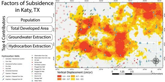
The decomposed InSAR line of sight vertical displacement results (Figure 7) show a distinct circular pattern of downward deformation around the city of Katy, up to 1.4 cm/year in the key areas mentioned above.
The generalized linear regression results (Figure 8) show the highest correlation between the GNSS-derived vertical displacement rates and population growth, total developed area, and groundwater pumping. The values range from 0 to 1 and can be interpreted simply as the percentage of variation in the dependent variable that can be explained by each individual independent variable.
5. Discussion
5.1. Groundwater Withdrawal
Excessive groundwater extraction from the Gulf Coast Aquifer has been determined to play a leading role in subsidence along the Gulf Coast and the establishment of regulatory agencies in the form of groundwater conservation districts has been an attempt to address the problem. Despite regulation, the amount of groundwater extraction has continued to rise (Figure 9).
Although there is evidence that subsidence in historically critical areas has slowed down or halted [50], and even reversed [10] in some cases, there is still active subsidence in the Gulf Coast region, with new areas becoming critical subsidence centers that need to be addressed. For example, in studies conducted over the past decade, the critical subsidence hotspots in the Houston area were identified in the north and north-east [15,25,51,52]. These areas included Spring, the Woodlands, and Montgomery County. A report [10] published by the Harris–Galveston Subsidence District on subsidence with a project timeline of 2019–2021 suggests that the maximum subsidence rate has now moved from the north and north-east to the Katy area in the west. This trend is consistent with subsidence centers following population growth [2]. There is a direct correlation between population growth and groundwater extraction to meet increased demands, and has been documented in particular for the greater Houston area [53]. This correlation is also evident for the Katy area (Figure 9). The regression analysis results give groundwater extraction an value of 0.91, suggesting that it is still one of the primary contributors to subsidence in the area.
5.2. Hydrocarbon Withdrawal
Along with excessive groundwater abstraction, the withdrawal of hydrocarbons in the form of oil and natural gas is considered to be a major contributor to subsidence in the Greater Houston area [54,55,56,57]. The history of subsidence attributed to hydrocarbon extraction in this area dates back to 1918 in the Goose Creek Oil Field, where up to 11 cm/year of subsidence was observed [58]. Annual production data for oil and gas in the Katy area have a high correlation (0.87 and 0.85 values, respectively) with the GNSS vertical displacement. Despite a decline in annual oil and gas production since 2014 (Figure 9), there are numerous oil and gas wells within our study area (Figure 10) that are significant contributors to subsidence in the area.
5.3. Total Developed Area
Developed or urbanized areas are composed of a variety of impervious surfaces that significantly alter or disrupt local hydrological processes. These surfaces, such as concrete pavement, roads, and rooftops, hinder the natural infiltration of water into the soil, resulting in increased surface runoff and reduced groundwater recharge [59,60,61,62,63].
One of the primary effects of impervious surfaces is the alteration of the natural flow patterns of water. The rapid runoff generated from these surfaces can overwhelm drainage systems and natural waterways, leading to increased flood risk, particularly during heavy rainfall events [60,63]. Disruption of the natural ground infiltration process due to impervious surfaces reduces the amount of water that replenishes aquifers and increases surface runoff [61,64,65].
Between 2013 and 2022, the amount of developed area has almost doubled in the Katy area (Figure 9). Furthermore, the majority of this development has replaced pasture and herbaceous land.
The spatial distribution of these changes is determined using the classified 2013 and 2020 Landsat images with the compute change raster function in ArcGIS Pro (Figure 11).
The value for total developed area in the generalized linear regression analysis is 0.95, making it one of the most influential variables with respect to the GNSS vertical displacement measurements.
5.4. Population
The highest value in the generalized linear regression analysis is 0.99 assigned to population. A fast population growth rate leads to an increase in factors that directly influence subsidence such as groundwater extraction and land development to meet demand. Furthermore, urbanization leads to other changes in water demand based on economic development and changes in the efficiency of water use [68]. As such, population growth is the biggest driving factor in subsidence based on how strongly it influences other contributors that have a direct physical impact on subsidence.
5.5. Risk to Infrastructure
Infrastructure most susceptible to damage from the effects of subsidence is located in areas where there is a steep gradient in the line of sight velocity. Differential subsidence has been shown to cause surficial fracturing and faulting [69,70]. We calculate an InSAR deformation gradient to determine the areas that are most at risk of infrastructure damage (Figure 12). Previous studies have shown that an InSAR gradient map can be an effective tool in determining the areas that require careful monitoring for infrastructure damage [69,71].
In summary, in this work, for the first time, full resolution InSAR data are analyzed to assess and understand subsidence in Katy, a sprawling suburban area located west of Houston. Population growth, extensive groundwater withdrawal, and land-use changes associated with constructing new structures are the main drivers of subsidence in this region. Hydrocarbon production is an important driver in some parts of Texas, but production of oil and gas is on the decline in the Katy area. Recent studies support the findings of this work. For example, Younas et al. analyzed data for the fifty-six counties along the Gulf Coast of Texas, including Katy. They suggested population growth, groundwater withdrawal, and hydrocarbon extraction as the main drivers [72]. Similarly, our previous work on statistical analysis of InSAR time series data of the greater Houston area from 2016 to 2020 suggested groundwater pumping to be the primary driver of subsidence in the Katy area [2].
6. Conclusions
The Greater Houston area has a long history of subsidence primarily driven by groundwater pumping and hydrocarbon extraction. While groundwater extraction continues to be one of the main drivers of subsidence, we found the growth of population and expansion of developed areas to be the primary contributors to subsidence in the Katy area. Between 2013 and 2022, the developed areas in Katy nearly doubled, predominantly replacing pasture and herbaceous land, which may have significant implications for future subsidence patterns.
It is important to note that although hydrocarbon production has historically influenced subsidence trends in some parts of Texas, the Katy area has experienced a steady decline in production of oil and gas over the past few years. This has led to a lower subsidence contribution from hydrocarbon production activities in the Katy area.
Recent studies found that the main hotspot for subsidence in the Greater Houston area has shifted in recent years from Spring and the Woodlands in the north to Katy in the west, and our research provides further insight into the rates and spatial distribution of this deformation. Our InSAR analysis identifies key hotspots of subsidence within the Katy area with a subsidence rate of up to 1.4 cm/yr from 2017 to 2022. Furthermore, we determined areas most susceptible to infrastructure damage and development of surficial fractures and strongly recommend monitoring of critical infrastructure in these areas.
This study highlights the multifaceted nature of subsidence in this region. It is evident that urban expansion and groundwater extraction demand strategic consideration to mitigate the effects of subsidence. Our findings emphasize the need for proactive planning, sustainable urban development, and comprehensive management strategies to effectively address the complex issue of subsidence within the Katy area.
Author Contributions
O.T.: data curation, formal analysis, investigation, validation, visualization, writing—original draft, writing—review and editing. S.D.K.: conceptualization, project administration, supervision, writing—review and editing. All authors have read and agreed to the published version of the manuscript.
Funding
This research received no external funding.
Data Availability Statement
Data can be requested by emailing the corresponding author.
Acknowledgments
O.T. would like to thank Muhammad Younas for his help in finding data; Kristofer Lasko, from the United States Army Corps of Engineers’ Geospatial Research Laboratory for consultation.
Conflicts of Interest
The authors declare no conflict of interest.
References
- National Oceanic and Atmospheric Administration What Is Subsidence? Available online: https://oceanservice.noaa.gov/facts/subsidence.html (accessed on 15 February 2023).
- Khan, S.D.; Gadea, O.C.A.; Tello Alvarado, A.; Tirmizi, O.A. Surface Deformation Analysis of the Houston Area Using Time Series Interferometry and Emerging Hot Spot Analysis. Remote Sens. 2022, 14, 3831. [Google Scholar] [CrossRef]
- Jones, C.E.; An, K.; Blom, R.G.; Kent, J.D.; Ivins, E.R.; Bekaert, D. Anthropogenic and Geologic Influences on Subsidence in the Vicinity of New Orleans, Louisiana. J. Geophys. Res. Solid Earth 2016, 121, 3867–3887. [Google Scholar] [CrossRef]
- Subsidence Overview. Available online: https://hgsubsidence.org/science-research/what-is-subsidence/ (accessed on 10 May 2023).
- Solarski, M.; Machowski, R.; Rzetala, M.; Rzetala, M.A. Hypsometric Changes in Urban Areas Resulting from Multiple Years of Mining Activity. Sci. Rep. 2022, 12, 2982. [Google Scholar] [CrossRef]
- Zheng, L.; Zhu, L.; Wang, W.; Guo, L.; Chen, B. Land Subsidence Related to Coal Mining in China Revealed by L-Band InSAR Analysis. Int. J. Environ. Res. Public Health 2020, 17, 1170. [Google Scholar] [CrossRef]
- Nádudvari, Á. Using radar interferometry and SBAS technique to detect surface subsidence relating to coal mining in Upper Silesia from 1993–2000 and 2003–2010. Environ. Soc.-Econ. Stud. 2016, 4, 24–34. [Google Scholar] [CrossRef]
- Hettema, M. Analysis of Mechanics of Fault Reactivation in Depleting Reservoirs. Int. J. Rock Mech. Min. Sci. 2020, 129, 104290. [Google Scholar] [CrossRef]
- Zilkoski, D.B.; Hall, L.W.; Mitchell, G.J.; Kammula, V.; Singh, A.; Chrismer, W.M.; Neighbors, R.J. The Harris-Galveston Coastal Subsidence District/ National Geodetic Survey Automated Global Positioning System Subsidence Monitoring Project. In Proceedings of the US Geological Survey Subsidence Interest Group Conference, Reston, VA, USA, 1 November 2003. [Google Scholar]
- Qu, F.; Lu, Z. Mapping Deformation Over Greater Houston Using InSAR. Available online: https://hgsubsidence.org/wp-content/uploads/2022/11/InSAR-Final-Report-2019-2021.pdf (accessed on 10 May 2023).
- Gambolati, G.; Teatini, P.; Ferronato, M. Anthropogenic Land Subsidence. In Encyclopedia of Hydrological Sciences; Anderson, M.G., McDonnell, J.J., Eds.; John Wiley & Sons: Hoboken, NJ, USA, 2006. [Google Scholar] [CrossRef]
- Candela, T.; Koster, K. The Many Faces of Anthropogenic Subsidence. Science 2022, 376, 1381–1382. [Google Scholar] [CrossRef]
- Herrera-García, G.; Ezquerro, P.; Tomás, R.; Béjar-Pizarro, M.; López-Vinielles, J.; Rossi, M.; Mateos, R.M.; Carreón-Freyre, D.; Lambert, J.; Teatini, P.; et al. Mapping the Global Threat of Land Subsidence. Science 2021, 371, 34–36. [Google Scholar] [CrossRef]
- Petersen, C.; Turco, M.J.; Vinson, A.; Turco, J.A.; Petrov, A.; Evans, M. Groundwater Regulation and the Development of Alternative Source Waters to Prevent Subsidence, Houston Region, Texas, USA. Proc. Int. Assoc. Hydrol. Sci. 2020, 382, 797–801. [Google Scholar] [CrossRef]
- Liu, Y.; Wang, G.; Yu, X.; Wang, K. Sentinel-1 InSAR and GPS-Integrated Long-Term and Seasonal Subsidence Monitoring in Houston, Texas, USA. Remote Sens. 2022, 14, 6184. [Google Scholar] [CrossRef]
- Liu, Y.; Li, J.; Fang, Z.N. Groundwater Level Change Management on Control of Land Subsidence Supported by Borehole Extensometer Compaction Measurements in the Houston-Galveston Region, Texas. Geosciences 2019, 9, 223. [Google Scholar] [CrossRef]
- Braun, C.L.; Ramage, J.K. Status of Groundwater-Level Altitudes and Long-Term Groundwater-Level Changes in the Chicot, Evangeline, and Jasper Aquifers, Houston-Galveston Region, Texas; U.S. Geological Survey: Reston, VA, USA, 2020. [Google Scholar]
- Ellis, J.; Knight, J.E.; White, J.T.; Sneed, M.; Hughes, J.D.; Ramage, J.K.; Braun, C.L.; Teeple, A.; Foster, L.K.; Rendon, S.H.; et al. Hydrogeology, Land-Surface Subsidence, and Documentation of the Gulf Coast Land Subsidence and Groundwater-Flow (GULF) Model, Southeast Texas, 1897–2018; Professional Paper; U.S. Geological Survey: Reston, VA, USA, 2023; Volume 1877, p. 432. [Google Scholar]
- Miller, M.M.; Shirzaei, M. Land Subsidence in Houston Correlated with Flooding from Hurricane Harvey. Remote Sens. Environ. 2019, 225, 368–378. [Google Scholar] [CrossRef]
- Kelley, V.; Turco, M.; Deeds, N.; Petersen, C.; Canonico, C. Assessment of Subsidence Risk Associated with Aquifer Storage and Recovery in the Coastal Lowlands Aquifer System, Houston, Texas, USA. Proc. Int. Assoc. Hydrol. Sci. 2020, 382, 487–491. [Google Scholar] [CrossRef]
- Campbell, M.; Campbell, M.; Wise, H.M. Growth Faulting and Subsidence in the Houston, Texas Area: Guide to the Origins, Relationships, Hazards, Potential Impacts and Methods of Investigation: An Update; Institute of Environmental Technology: Houston, TX, USA, 2015. [Google Scholar]
- Weaver, P.; Sheets, M.M. Active Faults, Subsidence, and Foundation Problems in the Houston, Texas, Area: Field Excursion No. 5, November 11 and 15, 1962; Houston Geological Society: Houston, TX, USA, 1962. [Google Scholar]
- Holzer, T.L.; Gabrysch, R.K. Effect of Water-Level Recoveries on Fault Creep, Houston, Texas. Ground Water 1987, 25, 392–397. [Google Scholar] [CrossRef]
- Kreitler, C.W. Fault Control of Subsidence, Houston, Texas. Ground Water 1977, 15, 203–214. [Google Scholar] [CrossRef]
- Qu, F.; Lu, Z.; Kim, J.-W.; Zheng, W. Identify and Monitor Growth Faulting Using InSAR over Northern Greater Houston, Texas, USA. Remote Sens. 2019, 11, 1498. [Google Scholar] [CrossRef]
- Bird, D.; Burke, K.; Hall, S.; Casey, J. Tectonic Evolution of the Gulf of Mexico Basin. In Gulf of Mexico Origin, Waters, and Biota: Geology; Texas A&M University Press: College Station, TX, USA, 2011; Volume 3. [Google Scholar]
- Stover, S.C.; Weimer, P.; Ge, S. The Effect of Allochthonous Salt Evolution and Overpressure Development on Source Rock Thermal Maturation: A Two-Dimensional Transient Study in the Northern Gulf of Mexico Basin. Pet. Geosci. 2001, 7, 281–290. [Google Scholar] [CrossRef]
- Salvador, A. Late Triassic-Jurassic Paleogeography and Origin of Gulf of Mexico Basin. AAPG Bull. 1987, 71, 419–451. [Google Scholar] [CrossRef]
- Galloway, W. Chapter 15 Depositional Evolution of the Gulf of Mexico Sedimentary Basin. Sediment. Basins World 2008, 5, 505–549. [Google Scholar] [CrossRef]
- Winker, C.D. Cenozoic Shelf Margins, Northwestern Gulf of Mexico(*). Gulf Coast Assoc. Geol. Soc. 1982, 32, 427–448. [Google Scholar]
- Engelkemeir, R.M.; Khan, S.D. Lidar Mapping of Faults in Houston, Texas, USA. Geosphere 2008, 4, 170–182. [Google Scholar] [CrossRef]
- Aronow, S.; Fisher, W.L.; McGowen, J.H.; Barnes, V.E. Geologic Atlas of Texas, Houston Sheet; The University of Texas at Austin, Bureau of Economic Geology, Geologic Atlas of Texas: Houston, TX, USA, 1982. [Google Scholar]
- Lissie Formation (TXQl;0). Available online: https://mrdata.usgs.gov/geology/state/sgmc-unit.php?unit=TXQl%3B0 (accessed on 12 July 2023).
- Khan, S.; Stewart, R.; Otoum, M.; Chang, L. A Geophysical Investigation of the Active Hockley Fault System near Houston, Texas. Geophysics 2013, 78, B177–B185. [Google Scholar] [CrossRef]
- Fattahi, H.; Agram, P.; Simons, M. A Network-Based Enhanced Spectral Diversity Approach for TOPS Time-Series Analysis. IEEE Trans. Geosci. Remote Sens. 2017, 55, 777–786. [Google Scholar] [CrossRef]
- Mirzaee, S.; Amelung, F.; Fattahi, H. Non-Linear Phase Inversion Package for Time Series Analysis. In Proceedings of the AGU Fall Meeting Abstracts 2019, San Francisco, CA, USA, 9–13 December 2019; p. G13C-0572. [Google Scholar]
- Mirzaee, S.; Amelung, F.; Fattahi, H. Non-Linear Phase Linking Using Joined Distributed and Persistent Scatterers. Comput. Geosci. 2023, 171, 105291. [Google Scholar] [CrossRef]
- Mirzaee, S.; Amelung, F. Volcanic Activity Change Detection Using SqueeSAR-InSAR and Backscatter Analysis. In Proceedings of the AGU Fall Meeting Abstracts 2018, Washington, DC, USA, 10–14 December 2018; p. G41B-0707. [Google Scholar]
- Yunjun, Z.; Fattahi, H.; Amelung, F. Small Baseline InSAR Time Series Analysis: Unwrapping Error Correction and Noise Reduction. Comput. Math. Geosci. 2019, 133, 104331. [Google Scholar] [CrossRef]
- Ansari, H.; De Zan, F.; Parizzi, A. Study of Systematic Bias in Measuring Surface Deformation With SAR Interferometry. IEEE Trans. Geosci. Remote Sens. 2021, 59, 1285–1301. [Google Scholar] [CrossRef]
- Ansari, H.; Zan, F.D.; Bamler, R. Sequential Estimator: Toward Efficient InSAR Time Series Analysis. IEEE Trans. Geosci. Remote Sens. 2017, 55, 5637–5652. [Google Scholar] [CrossRef]
- Ansari, H.; Zan, F.D.; Bamler, R. Efficient Phase Estimation for Interferogram Stacks. IEEE Trans. Geosci. Remote Sens. 2018, 56, 4109–4125. [Google Scholar] [CrossRef]
- Chen, C.W.; Zebker, H.A. Two-Dimensional Phase Unwrapping with Use of Statistical Models for Cost Functions in Nonlinear Optimization. J. Opt. Soc. Am. A 2001, 18, 338. [Google Scholar] [CrossRef]
- Ferretti, A.; Fumagalli, A.; Novali, F.; Prati, C.; Rocca, F.; Rucci, A. A New Algorithm for Processing Interferometric Data-Stacks: SqueeSAR. IEEE Trans. Geosci. Remote Sens. 2011, 49, 3460–3470. [Google Scholar] [CrossRef]
- Fialko, Y.; Simons, M.; Agnew, D. The Complete (3-D) Surface Displacement Field in the Epicentral Area of the 1999 MW7.1 Hector Mine Earthquake, California, from Space Geodetic Observations. Geophys. Res. Lett. 2001, 28, 3063–3066. [Google Scholar] [CrossRef]
- Wright, T.; Parsons, B.; Lu, Z. Toward Mapping Surface Deformation in Three Dimensions Using InSAR. Geophys. Res. Lett. 2004, 31, L01607. [Google Scholar] [CrossRef]
- Zhong, W.; Chu, T.; Tissot, P.; Wu, Z.; Chen, J.; Zhang, H. Integrated Coastal Subsidence Analysis Using InSAR, LiDAR, and Land Cover Data. Remote Sens. Environ. 2022, 282, 113297. [Google Scholar] [CrossRef]
- National Land Cover Database Class Legend and Description | Multi-Resolution Land Characteristics (MRLC) Consortium. Available online: https://www.mrlc.gov/data/legends/national-land-cover-database-class-legend-and-description (accessed on 23 May 2023).
- Regression Analysis Basics—ArcGIS Pro|Documentation. Available online: https://pro.arcgis.com/en/pro-app/latest/tool-reference/spatial-statistics/regression-analysis-basics.htm (accessed on 26 April 2023).
- Galloway, D.; Coplin, L.; Ingebritsen, S. Effects of Land Subsidence in the Greater Houston Area. Water Sci. Technol. Libr. 2003, 46, 187–204. [Google Scholar] [CrossRef]
- Qu, F.; Lu, Z.; Zhang, Q.; Bawden, G.W.; Kim, J.-W.; Zhao, C.; Qu, W. Mapping Ground Deformation over Houston–Galveston, Texas Using Multi-Temporal InSAR. Remote Sens. Environ. 2015, 169, 290–306. [Google Scholar] [CrossRef]
- Bawden, G.W.; Johnson, M.R.; Kasmarek, M.C.; Brandt, J.T.; Middleton, C.S. Investigation of Land Subsidence in the Houston-Galveston Region of Texas by Using the Global Positioning System and Interferometric Synthetic Aperture Radar, 1993–2000; Scientific Investigations Report; U.S. Geological Survey: Reston, VA, USA, 2012; 98p. [Google Scholar]
- Groundwater Decline and Depletion|U.S. Geological Survey. Available online: https://www.usgs.gov/special-topics/water-science-school/science/groundwater-decline-and-depletion (accessed on 17 May 2023).
- Younas, M.; Khan, S.D.; Qasim, M.; Hamed, Y. Assessing Impacts of Land Subsidence in Victoria County, Texas, Using Geospatial Analysis. Land 2022, 11, 2211. [Google Scholar] [CrossRef]
- Liu, Y.; Li, J.; Fang, Z.N.; Rashvand, M.; Griffin, T. The Secondary Consolidation (Creep) Due to Geohistorical Overburden Pressure in the Houston-Galveston Region, Texas. Proc. Int. Assoc. Hydrol. Sci. 2020, 382, 315–320. [Google Scholar] [CrossRef]
- Yu, J.; Wang, G. GPS-Derived Ground Deformation within the Gulf of Mexico Region Referred to a Stable Gulf of Mexico Reference Frame. Nat. Hazards Earth Syst. Sci. 2016, 16, 1583–1602. [Google Scholar] [CrossRef]
- Khorzad, K. Land Subsidence Along the Texas Gulf Coast Due to Oil and Gas Withdrawal. Environ. Geosci. 1999, 6, 157. [Google Scholar] [CrossRef]
- Pratt, W.E.; Johnson, D.W. Local Subsidence of the Goose Creek Oil Field. J. Geol. 1926, 34, 577–590. [Google Scholar] [CrossRef]
- Shuster, W.D.; Bonta, J.; Thurston, H.; Warnemuende, E.; Smith, D.R. Impacts of Impervious Surface on Watershed Hydrology: A Review. Urban Water J. 2005, 2, 263–275. [Google Scholar] [CrossRef]
- Sohn, W.; Kim, J.-H.; Li, M.-H.; Brown, R.D.; Jaber, F.H. How Does Increasing Impervious Surfaces Affect Urban Flooding in Response to Climate Variability? Ecol. Indic. 2020, 118, 106774. [Google Scholar] [CrossRef]
- Wang, Y.; Zhang, X.; Xu, J.; Pan, G.; Zhao, Y.; Liu, Y.; Liu, H.; Liu, J. Accumulated Impacts of Imperviousness on Surface and Subsurface Hydrology—Continuous Modelling at Urban Street Block Scale. J. Hydrol. 2022, 608, 127621. [Google Scholar] [CrossRef]
- Ramamurthy, P.; Bou-Zeid, E. Contribution of Impervious Surfaces to Urban Evaporation. Water Resour. Res. 2014, 50, 2889–2902. [Google Scholar] [CrossRef]
- Kaur, L.; Rishi, M.; Sharma, S.; Khosla, A. Impervious Surfaces an Indicator of Hydrological Changes in Urban Watershed: A Review. Open Access J. Environ. Soil Sci. 2019, 4, 469–473. [Google Scholar] [CrossRef]
- Kim, H.; Jeong, H.; Jeon, J.; Bae, S. The Impact of Impervious Surface on Water Quality and Its Threshold in Korea. Water 2016, 8, 111. [Google Scholar] [CrossRef]
- Giglou, A.N.; Nazari, R.; Jazaei, F.; Karimi, M. Assessing the Effects of Increased Impervious Surface on the Aquifer Recharge through River Flow Network, Case Study of Jackson, Tennessee, USA. Sci. Total Environ. 2023, 872, 162203. [Google Scholar] [CrossRef] [PubMed]
- Lu, J.C.-C.; Lin, F.T. Analysis of Elastic Consolidation Due to Fluid Extraction from a Cross-Anisotropic Poroelastic Half Space. In Proceedings of the EASEC-11—Eleventh East Asia-Pacific Conference on Structural Engineering and Construction, Taipei, Taiwan, 19–21 November 2008. [Google Scholar]
- Tkachenko, I.; Lytvynenko, T.; Hasenko, L.; Sorochuk, N. Streets and Urban Roads Surface Runoff Problems: A Case Study in the Poltava City, Ukraine. In Proceedings of the TRANSBALTICA XIII: Transportation Science and Technology, Vilnius, Lithuania, 15–16 September 2022; Prentkovskis, O., Yatskiv (Jackiva), I., Skačkauskas, P., Maruschak, P., Karpenko, M., Eds.; Springer International Publishing: Cham, Switzerland, 2023; pp. 576–585. [Google Scholar]
- Vörösmarty, C.J.; Green, P.; Salisbury, J.; Lammers, R.B. Global Water Resources: Vulnerability from Climate Change and Population Growth. Science 2000, 289, 284–288. [Google Scholar] [CrossRef]
- Cabral-Cano, E.; Osmanoglu, B.; Dixon, T.; Wdowinski, S.; Demets, C.; Cigna, F.; D’iaz-Molina, O. Subsidence and Fault Hazard Maps Using PSI and Permanent GPS Networks in Central Mexico. In Land Subsidence, Associated Hazards and the Role of Natural Resources Development; IAHS-AISH Publication: Wallingford, UK, 2010; Volume 339, pp. 255–259. [Google Scholar]
- Holzer, T.L.; Johnson, A.I. Land Subsidence Caused by Ground Water Withdrawal in Urban Areas. GeoJournal 1985, 11, 245–255. [Google Scholar] [CrossRef]
- Tirmizi, O.; Khan, S.D.; Mirzaee, S.; Fattahi, H. Hazard Potential in Southern Pakistan: A Study on the Subsidence and Neotectonics of Karachi and Surrounding Areas. Remote Sens. 2023, 15, 1290. [Google Scholar] [CrossRef]
- Younas, M.; Khan, S.; Tirmizi, O.; Hamed, Y. Geospatial Analytics of Driving Mechanism of Land Subsidence in Gulf Coast of Texas, United States. Sci. Total Environ. 2023, 902, 166102. [Google Scholar] [CrossRef] [PubMed]
Figure 1.
Study area with InSAR boundary and water wells displayed with reference regional faults and salt domes in the Greater Houston area [2].
Figure 1.
Study area with InSAR boundary and water wells displayed with reference regional faults and salt domes in the Greater Houston area [2].

Figure 2.
ISCE2 TOPS stack processor workflow. Raw data in the form of Sentinel 1 SLCs, precise or restituted orbit files, and a digital elevation model are loaded into the ISCE2 tops stack processor. Burst overlaps are extracted from secondary SLCs and geometrical offsets with the reference SLC are calculated. ESD method is used to estimate azimuth misregistration followed by calculation of range misregistration. Geometrical offsets are calculated between all secondary SLCs and stack reference using orbit and DEM files, precise co-registration is performed, and bursts are merged back into full SLCs.

Figure 3.
MiaplPy (red boxes) and MintPy (green boxes) workflow. The stack of co-registered SLCs and geometry files produced by the Sentinel-1 tops stack processor in ISCE are loaded at full resolution into MiaplPy. Miaplpy is used for non-linear phase linking followed by generation and unwrapping of interferograms. The unwrapped interferogram stack is loaded into MintPy for unwrapping error corrections. The corrected interferograms are then loaded into MiaplPy to convert the estimated unwrapped timeseries into a range–change time series. The range–change time series is then imported into MintPy for time series error corrections, velocity estimation, and geocoding.

Figure 4.
(top) Landsat 8 image clipped to study area. (bottom) Clipped Landsat image classified by land-use/land cover type. Each Landsat image is processed using ArcGIS Pro’s classify pixels using deep learning tool with ESRI’s pre-trained deep learning model. Once all the images are classified, we run the zonal geometry tool on the classified image for each year to obtain the total area for every land cover class.

Figure 5.
LOS velocity change results from InSAR processing for ascending (top) and descending (bottom) tracks. Letters A–D correspond with key areas displayed in greater detail in Figure 6. The descending track results have a more discontinuous distribution of points most likely due to descending track SLC images being captured later in the day when the atmosphere has more pollutants, leading to lack of coherence between images. Low coherence areas are masked out during InSAR processing for reliability.

Figure 6.
LOS velocity change results corresponding to the key areas labeled A through D in Figure 5 for ascending (top) and descending (bottom) tracks. The majority of the Katy area appears to have a displacement rate between −0.4 to −0.8 cm/year, some key areas show deformation rates of up to −1.4 cm/year.

Figure 7.
Vertical displacement results with inverse distance weighted interpolation and resampling to 100 m resolution. A distinct circular pattern of downward deformation around the city of Katy, up to 1.4 cm/year can be seen.
Figure 7.
Vertical displacement results with inverse distance weighted interpolation and resampling to 100 m resolution. A distinct circular pattern of downward deformation around the city of Katy, up to 1.4 cm/year can be seen.

Figure 8.
Generalized linear regression results. The bottom left displays scatterplots of variable relationships, the middle diagonal displays histograms, and the upper right displays R-squared values between variables. The values range from 0 to 1 and can be interpreted simply as the percentage of variation in the dependent variable that can be explained by each individual independent variable. The boxes range in color from low values (yellow) to high values (red) to help visualize the distribution of values. Negligible values have no background color. The generalized linear regression results show the highest correlation between the GNSS-derived vertical displacement rates and population growth, total developed area, and groundwater pumping.

Figure 9.
Time series plots of each variable used in the generalized linear regression workflow.

Figure 10.
Hydrocarbon wells in the Katy area. There is a wide distribution of both oil and gas extraction wells ranging from dry holes to active production and plugged wells. There is a high concentration of oil and gas wells in the east and northeast portion of the study area that correspond to some of the areas with the highest subsidence rate in Katy.

Figure 11.
Change in land cover from 2013 to 2022. (top) Pixels that were classified as natural/vegetated cover in 2013 but a different class in 2022. (bottom) Pixels that changed from any other class to developed area by 2022.
Figure 11.
Change in land cover from 2013 to 2022. (top) Pixels that were classified as natural/vegetated cover in 2013 but a different class in 2022. (bottom) Pixels that changed from any other class to developed area by 2022.

Figure 12.
InSAR deformation gradient highlighting areas most at risk for infrastructure damage in red.
Figure 12.
InSAR deformation gradient highlighting areas most at risk for infrastructure damage in red.


Table 1.
Data used in this study and sources.
| Data | Source | Purpose | Method |
|---|---|---|---|
| Sentinel-1 SLC | Alaska Satellite Facility (ASF) Vertex https://search.asf.alaska.edu/, accessed on 17 May 2022 | Surface deformation | InSAR |
| Copernicus 30 m DEM | European Space Agency (ESA) https://spacedata.copernicus.eu/, accessed on 18 May 2022 | Surface deformation | InSAR |
| GNSS Vertical Displacement Data | Global Navigation Satellite Systems (GNSS) http://geodesy.unr.edu/, accessed on 11 April 2023 | Subsidence rate | GLR |
| Population Records | Texas A & M University Texas Real Estate Research Center https://www.recenter.tamu.edu/, accessed on 20 March 2023 | Subsidence contribution | GLR |
| Groundwater Pumping Records | Texas Water Development Board (TWDB) https://www3.twdb.texas.gov/, accessed on 20 March 2023 | Subsidence contribution | GLR |
| Hydrocarbon Production Records | Railroad Commission of Texas https://www.rrc.texas.gov/, accessed on 23 March 2023 | Subsidence contribution | GLR |
| Precipitation Records | Southern Regional Climate Center (SRCC) https://www.srcc.tamu.edu/, accessed on 22 March 2023 | Subsidence contribution | GLR |
| Landsat 8/9 Level 2 Surface Reflectance Imagery | United States Geological Survey (USGS) Earth Explorer https://earthexplorer.usgs.gov/, accessed on 20 April 2023 | Land-use classification | ArcGIS Pro |
| Landsat Land Cover Classification Deep Learning Model | ESRI https://arcg.is/HLKyf, accessed on 23 March 2023 | Land-use classification | ArcGIS Pro |
| Total Developed Area | Generated using Landsat imagery and ESRI’s pre-trained model | Subsidence contribution | GLR |
Disclaimer/Publisher’s Note: The statements, opinions and data contained in all publications are solely those of the individual author(s) and contributor(s) and not of MDPI and/or the editor(s). MDPI and/or the editor(s) disclaim responsibility for any injury to people or property resulting from any ideas, methods, instructions or products referred to in the content. |
© 2023 by the authors. Licensee MDPI, Basel, Switzerland. This article is an open access article distributed under the terms and conditions of the Creative Commons Attribution (CC BY) license (https://creativecommons.org/licenses/by/4.0/).
Share and Cite
MDPI and ACS Style
Tirmizi, O.; Khan, S.D. Factors of Subsidence in Katy, Texas, USA. Remote Sens. 2023, 15, 4424. https://0-doi-org.brum.beds.ac.uk/10.3390/rs15184424
AMA Style
Tirmizi O, Khan SD. Factors of Subsidence in Katy, Texas, USA. Remote Sensing. 2023; 15(18):4424. https://0-doi-org.brum.beds.ac.uk/10.3390/rs15184424
Chicago/Turabian StyleTirmizi, Osman, and Shuhab D. Khan. 2023. "Factors of Subsidence in Katy, Texas, USA" Remote Sensing 15, no. 18: 4424. https://0-doi-org.brum.beds.ac.uk/10.3390/rs15184424
Note that from the first issue of 2016, this journal uses article numbers instead of page numbers. See further details here.