
Hyperspectral Image Super-Resolution via Adaptive Factor Group Sparsity Regularization-Based Subspace Representation


1
The Chongqing Key Laboratory of Image Cognition, Chongqing University of Posts and Telecommunications, Chongqing 400065, China
2
The Chongqing Engineering Research Center for Spatial Big Data Intelligent Technology, Chongqing University of Posts and Telecommunications, Chongqing 400065, China
3
The School of Computer Science and Cyber Engineering, Guangzhou University, Guangzhou 510006, China
*
Author to whom correspondence should be addressed.
Remote Sens. 2023, 15(19), 4847; https://0-doi-org.brum.beds.ac.uk/10.3390/rs15194847
Submission received: 2 September 2023
/
Revised: 30 September 2023
/
Accepted: 5 October 2023
/
Published: 7 October 2023
(This article belongs to the Section Remote Sensing Image Processing)
Abstract
:Hyperspectral image (HSI) super-resolution is a vital technique that generates high spatial-resolution HSI (HR-HSI) by integrating information from low spatial-resolution HSI with high spatial-resolution multispectral image (MSI). However, existing subspace representation-based methods face challenges, including adaptive subspace dimension determination, inadequate spectral correlation capture, and expensive computation. In this paper, we propose a novel factor group sparsity regularized subspace representation (FGSSR)-based method for HSI super-resolution that can simultaneously address these issues encountered in previous methods. Specifically, by incorporating the factor group sparsity regularization into the subspace representation model, we first propose an FGSSR model to capture the spectral correlation property of the HR-HSI. The key advantage of FGSSR lies in its equivalence to the Schatten-p norm and its adaptive determination of the accurate subspace dimension, enabling it to capture spectral correlation more effectively. To preserve the spatial self-similarity prior in the HR-HSI, the tensor nuclear norm regularization on the low-dimensional coefficients is also incorporated into the proposed FGSSR-based model. Finally, an effective proximal alternating minimization-based algorithm is developed to solve the FGSSR-based model. Experimental results on the simulated and real datasets demonstrate that the proposed FGSSR-based method outperforms several state-of-the-art fusion methods with significant improvements.
1. Introduction
Hyperspectral (HS) imaging is an advanced technology that enables the acquisition of a high-dimensional image dataset encompassing numerous diverse bands. Due to their rich spectral information, HS images (HSIs) have become extensively utilized for numerous earth observation tasks, such as image classification [1,2], ecosystem monitoring [3], and change detection [4]. Nevertheless, HS imaging sensors struggle to balance their spatial and spectral resolutions due to finite sun irradiation [5,6,7]. As a result, HSIs often prioritize spectral resolution over spatial resolution, restricting their applications in the study of land surface dynamics occurring in small areas [8,9,10]. Fortunately, multispectral (MS) imaging sensors generally outperform HS imaging sensors in terms of spatial resolution. This provides an opportunity to perform HSI super-resolution by integrating complementary information of the high spatial-resolution MS images (HR-MSIs) and the low spatial-resolution HSIs (LR-HSIs) captured from the same scene, resulting in the generation of the desired HR-HSIs. Current HSI super-resolution approaches are primarily categorized into three groups [11]: deep learning (DL)-based methods [12,13,14], matrix factorization-based methods [15,16], tensor-based methods [17,18,19].
The remarkable learning performance and effective computing capabilities of DL contributed to the development of DL-based HSI super-resolution techniques [13,20]. For example, the work in [21] designed a deep residual learning network for HSI super-resolution, which effectively learns the spectral prior by using the deep convolution neural network (CNN). The work in [14] presented a simple and efficient CNN architecture that can maintain the spatial and spectral specifics of the observations. The main benefit of these techniques lies in their ability to achieve satisfactory results by leveraging the powerful feature capturing capabilities of CNNs. However, it is worth noting that these methods are supervised and rely on a substantial amount of labeled samples to pretrain the CNN. In order to tackle this matter, numerous scholars have put forth unsupervised deep learning-based approaches [22,23]. For example, in work [22], an unsupervised and non-pretraining encoder–decoder architecture for HSI super-resolution was designed. However, these unsupervised methods may produce slightly worse results than the supervised methods.
Matrix factorization-based methods approximate the latent HR-HSI using a dictionary and its corresponding coefficients, assuming that every spectral component is able to be expressed as a composition of a small set of distinct spectral patterns. Within this theoretical framework, the primary focus centers around the precise estimation of both the dictionary and its accompanying coefficients. Several methods [24,25,26] estimated the dictionary and its corresponding coefficients using certain predetermined priors. For instance, Xue et al. [26] exploited the subspace low-rank priors in both spatial and spectral dimensions to accomplish HSI super-resolution. In addition, previous studies [27,28] successfully addressed the HSI super-resolution problem through the utilization of spatial structures inherent in HR-HSI. For example, Simoes et al. [27] attempted to capture the spatial self-similarity features through the total variation regularization. However, fusion approaches based on matrix factorization encounter difficulties in fully leveraging the spatial and spectral correlations of the HR-HSI due to their approach of unfolding the high-dimensional HSI into matrices without considering its underlying data structure. As a result, those methods often yield unsatisfactory fusion outcomes [29,30].
Given that HSI is a three-order tensor, methods based on tensor theory have gained significant attention in addressing the HSI super-resolution problem [31]. These methods address the HSI super-resolution problem using various tensor decompositions, including tensor ring decomposition [17,18,19,31], tensor train decomposition [9], Canonical polyadic decomposition [32,33,34], and Tucker decomposition [8,17,29,30,35,36,37], while incorporating specific priors. For example, Dian et al. [35] developed an HSI super-resolution approach via Tucker decomposition, which reconstructs the latent HR-HSI by utilizing dictionary learning and sparse coding. He et al. [18] developed a coupled tensor ring factorization-based approach that can simultaneously learn tensor ring core tensors from the observations for reconstructing the latent HR-HSI. Although these tensor decomposition-based methods have yielded promising performances, they still encounter certain challenges and limitations. One of the challenges is the high computational cost associated with representing the strong spectral and spatial correlations in the original HSI domain through tensor decompositions, particularly when dealing with a large number of bands in HSI [6].
The spectral bands in the HR-HSI exhibit a strong correlation and typically reside inside a subspace of reduced dimensionality [38]. This implies that HSI super-resolution is able to be modeled by projecting the high-dimensional HR-HSI into a lower-dimensional subspace. This strategy can largely decrease the computing complexity and enhance the spectral correlation property [6]. Recently, many HSI super-resolution methods [6,38,39,40] have been proposed through subspace representation. Xu et al. [6] exploited a tensor subspace representation to effectively leverage the nonlocal and global spectral–spatial low-rank priors to accomplish HSI super-resolution. Xing et al. [39] presented a fusion approach based on variational tensor subspace decomposition. This method effectively captures the distinctions and interrelationships among the three modes of the HR-HSI. To exploit both the global and nonlocal priors, Xu et al. [40] developed a tensor ring decomposition-based approach that blends spectral subspace learning, nonlocal similarity learning, and the tensor nuclear norm. Compared with matrix/tensor decomposition-based methods, subspace representation-based methods project the high-dimensional HR-HSI into the low-dimensional spectral subspace, consuming less computational complexity and generating better results. However, the current subspace representation-based methods often encounter challenges in adaptively selecting the appropriate subspace dimension, making them highly sensitive to changes in subspace dimension and affecting their overall performance.
To tackle the aforementioned concerns, this study develops a factor group sparsity regularized subspace representation-based method for HSI super-resolution. Specifically, we first propose a factor group sparsity regularized subspace representation (FGSSR) model, which automatically selects the appropriate subspace dimension, resulting in a precise depiction of the high spectral correlations in the latent HR-HSI. The proposed FGSSR model has several advantages that can be summarized as follows: (1) FGSSR is established based on subspace representation framework, resulting in an optimization process with low computational cost. (2) FGSSR is rank-revealing by seeking to minimize the number of nonzero frontal slices of the coefficient tensor. Thus, it provides a solution to the challenge of adaptively selecting the appropriate subspace dimension faced by previous subspace representation methods. (3) FGSSR corresponds to the Schatten-p norm, allowing it the selection of a subspace dimension that is closer to the true rank of the latent HR-HSI compared to the nuclear norm. Under the FGSSR framework, the depiction of the spatial structure prior in the high-dimensional HR-HSI domain can be translated into an exploration of the low-dimensional coefficient domain. Driven by the efficacy of the tensor nuclear norm (TNN) [41], we impose it on the low-dimensional coefficient tensor to capture and retain the spatial information inherent in the latent HR-HSI. Furthermore, we design an effective optimization algorithm under the proximal alternating minimization (PAM) framework to address our FGSSR-based HSI super-resolution model. This study makes several notable contributions in the following areas:
- We propose an FGSSR-based HSI super-resolution method that overcomes the sensibility of the subspace dimension determination of earlier subspace representation-based methods. Specifically, by incorporating factor group sparsity regularization into subspace representation, FGSSR becomes rank-revealing, enabling it to adaptively and accurately approximate the subspace dimension to the rank of the latent HR-HSI.
- The FGSSR-based method utilizes the FGSSR model to explore spectral correlation and employs TNN regularization to capture spatial self-similarity in the latent HR-HSI. FGSSR can adaptively and effectively capture the high spectral correlation by fully leveraging the advantages of subspace representation and the Schatten-p norm while mitigating their limitations. TNN regularization on the low-dimensional coefficients can effectively capture the spatial self-similarity and facilitate efficient computations through dimensionality reduction.
- An effective PAM-based algorithm is developed with the aim of addressing the FGSSR-based model. Extensive studies carried out with simulated and real-world datasets reveal that our FGSSR-based method outperforms the state-of-the-art (SOTA) HSI super-resolution methods in both quantitative and visual judgements.
The ensuing section of this paper is structured as follows: Section 2 introduces the related work. Section 3 presents the FGSSR-based method, outlining its key features and methodology. Section 4 and Section 5 present the experimental results and model discussions, respectively. Finally, Section 6 concludes this paper and discusses the potential future research directions.
2. Related Work
2.1. Notations
We let be a three-dimensional tensor. is the ith frontal slice of , denoted . Mode-n unfolding operator of is given by , and can be retrieved by reversing this process as . The norm of is represented as , the Frobenius norm is represented as , and the norm is denoted by . is the outcome of performing the fast Fourier transformation (FFT) on along the third dimension, denoted as . Likewise, can be retrieved through inverse FFT, denoted as . Additionally, we define a pair of unfolding–folding operators, that is,
Definition 1
Definition 2
(Orthogonal Tensor [42]). An orthogonal tensor is a special type of tensor that satisfies the following conditions: , where and are the identity tensor and the conjugate transpose of , respectively.
Theorem 1
(Tensor Singular Value Decomposition (t-SVD) [42]).
t-SVD decomposes as
where and are orthogonal, and is f-diagonal.
Definition 3
(TNN [41]). Let tensor , with its t-SVD given by . The TNN of tensor , denoted as , is the aggregate of the singular values of all frontal slice of tensor , that is,
where and are the block diagonal matrices of and , respectively. Following Definition 3, the TNN can be accomplished efficiently by employing a single matrix SVD, as opposed to the use of the complex t-SVD method for obtaining .
Definition 4
(Singular Value Thresholding (SVT) [41]). The SVT operator performed on tensor is given by
where denotes the SVT operator, and τ is a positive scalar.
Theorem 2
Definition 5
(Schatten-p Norm [44]). For any matrix , its Schatten-p norm () can be defined as
where is the ith singular value of . In special cases at the boundaries, the Schatten-p norm simplifies into the nuclear norm when , and it reduces to the rank function when p is 0. When , the Schatten-p norm can be seen as a rank approximation lying between rank function and nuclear norm.
Theorem 3
([45]). For any matrix having the rank , it can be decomposed into two low-dimensional matrices and ,
where is the norm, denotes the Schatten-p norm of with , and denotes the ith singular of . Let the SVD of denote . When and , equality holds in Equation (8). Here, the low-rank approximation of (8) is called the factor group sparsity (FGS) regularizer.
2.2. Problem Formulation
(1) Observation Model: is the observed LR-HSI, which contains a wealth of spectral information. Current HSI super-resolution techniques mainly rely on the assumption that the LR-HSI is the spatially degraded version of the latent HR-HSI [39,46,47]. However, this assumption may not be totally justifiable due to the fact that the blur kernel is often unknown in real-world scenarios. To eliminate the need for an empirical blur kernel, this paper employs interpolation technology to upsample the observed LR-HSI, resulting in an upsampled LR-HSI , which can be represented as the combination of the latent HR-HSI and the difference image , that is,
where denotes the noise within the upsampled LR-HSI.
The observed HR-MSI contains a rich amount of spatial structure information. It can be considered the spectrally degraded form of the latent HR-HSI , i.e.,
where and represent the spectral response and noise in the observed HR-MSI, respectively.
(2) HSI Super-resolution Model: Indeed, directly reconstructing the latent HR-HSI from the observations is ill-posed. To achieve a robust reconstruction of the desired HR-HSI, we can employ the maximum a posteriori approach to incorporate regularization models and convert the ill-posed issue into a well-posed one. In addition, our previous work [48] has demonstrated that the gradients along the horizontal, vertical, and spectral modes of the difference image follow hyper-Laplacian distributions which can be depicted by norm. Therefore, we impose an norm on the gradients of to construct the spectral fidelity term. Therefore, HSI super-resolution model is given by
where the combination of the first two terms is the spectral fidelity term, and the third term is the spatial fidelity term. is a regularizer that depicts the potential property of the HR-HSI. is the norm, and represents the gradient operators along the mode-n. , , and w are positive parameters used to achieve a balance between the functions involved in the fusion process. The norm-based spectral fidelity term can skip the empirical blur kernel and reduce the computing complexity.
3. Proposed FGSSR-Based Method
In this section, we present an FGSSR-based method for fusing the LR-HSI and HR-MSI to generate the target HR-HSI. In this method, we first propose a FGSSR model that combines the subspace learning of a low-dimensional spectral subspace with the imposition of group sparsity regularization on a low-dimensional coefficient tensor to depict the high spectral correlations of HS-HSI. The proposed FGSSR model offers several advantages, including enhanced rank minimization, automatic subspace dimension selection, and low computational cost. These advantages allow us adaptive and effective capture of the high spectral correlations. Furthermore, since each frontal slice of the coefficient tensor can be regarded as the eigen-image [38], we also introduce TNN regularization on the low-dimensional coefficient tensor to depict the spatial self-similarity prior, which offers high efficiency while successfully maintaining the spatial features. The flowchart of the proposed FGSSR-based method is demonstrated in Figure 1.
3.1. Subspace Learning
For the latent HR-HSI, there is typically a significant correlation among spectral vectors. This indicates that spectral vectors in the latent HR-HSI often reside within a low-dimensional subspace [38,40,49]. Hence, the latent HR-HSI can be approximated by adopting a subspace representation strategy, that is,
where and represent the spectral subspace and its coefficients, respectively. Notably, the subspace dimension is significantly smaller than , which indicates that the spectral bands reside inside a low-dimensional subspace. This reduction in dimensionality drastically improves computational efficiency. However, the effectiveness of Subspace representation model (12) heavily relies on accurately determining the appropriate subspace dimension , namely the number of the frontal slices of . Therefore, the subspace dimension should be precisely chosen to approximate the rank of (i.e., the unfolding matrix of along the 3rd dimension) as closely as possible. Motivated by the FGS regularizer (8), we define a factor group sparsity regularized subspace representation (FGSSR) model (see Figure 2) for HSI super-resolution, that is,
Based on Theorem 3, FGSSR is equivalent to the Schatten-p norm when and , where is the unfolding matrix of along the third dimension, , , and come from the SVD of , i.e., . From Observation model (9), the upsampled LR-HSI consists of three components: the latent HR-HSI, the difference image, and noise. This suggests that a significant portion of spectral information of the latent HR-HSI is preserved in the upsampled LR-HSI. Consequently, it can be inferred that both LR-HSI and HR-HSI are situated inside the identical spectral subspace. As a result, the low-dimensional spectral subspace can be learned by SVD and Theorem 3 from the upsampled LR-HSI. We represent the upsampled LR-HSI using its SVD as follows:
where and are semiunitary, and is a diagonal matrix comprising the singular values sorted in a non-increasing manner. By saving the largest singular values and deleting the remaining () smallest ones from , a low-rank approximation of can be given by
Based on Theorem 3, the spectral subspace can be achieved by
Compared to Direct subspace representation model (12), the FGSSR model applies the group sparsity regularization to the coefficients , resulting in certain frontal slices in being quickly forced to zero during the iterative process. This allows the FGSSR model automatic reduction in the number of non-zero frontal slices and dynamic approximation of the rank of . Regarding to the spectral subspace , we make two remarks: (1) The spectral subspace is dynamic since its subspace dimension reduces with the reduction in the number of nonzero frontal slices of in the iterative optimization process. (2) As the iteration progresses, the FGSSR model dynamically reduces the number of columns in , allowing it the consideration as the spectral basis matrix of . This leads to inheriting the potential property of the latent HR-HSI . Therefore, the spatial property in the HR-HSI can be captured and modeled in its low-dimensional coefficient domain, which can reduce the computational complexity.
To sum up, the FGSSR model has the following advantages:
- Enhanced Rank Minimization: The FGSSR model corresponds to the Schatten-p norm, which enables it to provide a more precise approximation to rank minimization compared to the nuclear norm.
- Reduced Computational Complexity: Unlike other rank minimization problems that require SVD calculation at each iteration, the FGSSR model can be effectively solved through the soft-threshold shrinkage operator or tiny linear equations, resulting in enhanced computational efficiency. In addition, the FGSSR model employs the subspace learning strategy to learn the spectral subspace , which can also reduce the computational complexity.
- Automatic Subspace Dimension Selection: Compared to the direct subspace representation model (12), the FGSSR model (13) imposes the group sparsity regularization on the coefficients . This leads to the rapid elimination of specific frontal slices in during the iterative optimization process, automatically reducing the number of non-zero frontal slices (i.e., subspace dimension d), and dynamically approximating the rank r of .
3.2. Adaptive FGSSR-Based HSI Super-Resolution Model
By incorporating FGSSR model (13) into Model (11), we have
where is the FGSSR model, which serves to depict the high spectral correlations of the target HR-HSI . is a regularization term, which serves to capture the self-similarity property of the target HR-HSI . The idea of applying the TNN-based regularization to the low-dimensional coefficient tensor to capture the nonlocal self-similarity has been successfully used for HSI super-resolution [16,38,39], but often demands significant computational resources [50]. In this paper, the TNN is employed to capture the global spatial self-similarity property of the latent HR-HSI by directly performing on the low-dimensional coefficient tensor . This strategy offers a reduction in computational complexity while effectively preserving the image details. Moreover, through the subspace learning strategy, the spectral subspace is essentially known. Therefore, the proposed FGSSR-based HSI super-resolution model can ultimately be expressed as follows:
where , defined in (4), is the TNN regularization term.
In our proposed method, the spectral correlation property is adaptively and effectively depicted by the FGSSR model, and the spatial self-similarity property is effectively captured by imposing the TNN regularization on the low-dimensional coefficients . Specifically, we first propose the FGSSR model by combining the subspace learning of subspace with the imposition of group sparsity regularization on coefficients . The proposed FGSSR model offers several advantages, including enhanced rank minimization, automatic subspace dimension selection, and low computational cost. These advantages allow us adaptive and effective capture of the high spectral correlations. Furthermore, we introduce TNN regularization on the low-dimensional coefficients to depict the spatial self-similarity prior, which offers high efficiency while successfully maintaining the spatial features. Next, we design an efficient PAM-based algorithm for the proposed FGSSR-based HSI super-resolution model.
3.3. Optimization Algorithm
In this section, we employ the PAM framework [51] to address our Fusion model (18). We choose the PAM framework for two reasons. Firstly, the PAM framework has a proven ability that can guarantee convergence to a critical point given specific criteria. Secondly, the PAM framework provides us with an opportunity to update subspace dimension d at each PAM iteration. It should be noted that is initialized using the subspace learning strategy and subsequently updated only according to the subspace dimension d, which is determined by applying the group sparsity regularization to the coefficients during the iterative optimization process. In other words, is known with the subspace dimension d determined in each PAM iteration. As a result, solving Model (18) can be changed into an alternative optimization of the following subproblems:
where is the objective function implicitly defined in (18), is the variable predicted in the preceding iteration, and is a proximal parameter. Next, we address the two subproblems by using a two-step iterative scheme:
(1) Step 1: Optimization with respect to
From (19), we have
where is the coefficients determined in the preceding PAM iteration. To effectively deal with Problem (20), the alternating direction method of the multiplier (ADMM) framework [52] is adopted. By introducing the auxiliary valuables and , we obtain the augmented Lagrangian function as follows:
where and are Lagrange multipliers, and is a penalty parameter. The ADMM iteration process is given by
For the subproblem, we have
Problem (27) is quadratic, and it can be addressed via the Sylvester matrix equation
where .
For the subproblem, we have
The efficient solution to Problem (29) can be achieved through the utilization of the group sparse soft-threshold shrinkage operator. Subsequently, the closed-form solution for each frontal slice of can be derived as follows:
where , and .
The subproblem can be updated by
Based on the Definition 4 and Theorem 2, Problem (31) yields closed-form solution
where is the SVT operator.
To enhance comprehension, the process of optimizing subproblem (20) is succinctly outlined in Algorithm 1.
| Algorithm 1: ADMM Algorithm for Subproblem |
| Input: , , , , , , , , , , and |
| Initialization: Let , , . |
| 1: while not converged and do |
| 2: |
| 3: Update via (28). |
| 4: Update via (30). |
| 5: Update via (32). |
| 6: Update and via (25) and (26), respectively. |
| 7: Check the convergence condition: . |
| 8: end while |
| Output: Low-dimensional coefficient tensor |
(2) Step 2: Optimization with respect to
Updating the difference image is solved by
where represents the difference image determined in the preceding PAM iteration. Similar to the subproblem, we also employ ADMM to solve subproblem (33). By introducing the auxiliary valuable , we have
where is the Lagrangian multipliers. ADMM iterations follow this procedure:
The subproblem can be updated by
Problem (38) can be effectively solved by FFT strategy:
where is a tensor with all elements equal to 1.
For the subproblem, we have
Problem (40) that involves the norm is nonconvex. Here, we employ the generalized shrinkage/thresholding (GST) operation [53] to address Problem (40) due to its efficiency and low computational cost. Consequently, Nonconvex problem (40) yields the following solution:
where is the GST operator.
The process of optimizing the subproblem is succinctly outlined in Algorithm 2. Combining the solutions for the aforementioned two block subproblems, we derive the PAM algorithm (summarized in Algorithm 3) to solve the FGSSR-based model (18). Algorithm 3 has a strong capability to converge towards a critical point of the objective function, as proven in [51].
| Algorithm 2: ADMM Algorithm for Subproblem |
| Input: , , , , , , , , and |
| Initialization: Let , ,, . |
| 1: while not converged and do |
| 2: . |
| 3: Update via (39). |
| 4: Update , , via solving (41) with the GST operator. |
| 5: Update , , via (37). |
| 6: Check the convergence condition: . |
| 7: end while |
| Output: Difference image |
| Algorithm 3: PAM Algorithm for FGSSR-based Model |
| Input: , , , , , , w, , , , and |
| Initialize: , , ,
, where , , and come from the SVD of . |
| 1: while not converged and do |
| 2: . |
| 3: Update via solving (20) with Algorithm 1. |
| 4: Update via solving (33) with Algorithm 2. |
| 5: Update , where is the number of the nonzero frontal slices of |
| 6: Remove the zero frontal slices of . |
| 7: Update via (16). |
| 8: Check the convergence condition: . |
| 9: end while |
| Output: Target HR-HSI: |
3.4. Computational Complexity
Let us denote the acquired LR-HSI as and the acquired HR-MSI as . We let represent the subspace dimension. In Algorithm 3, the most computationally intensive parts involve solving the and subproblems. In Algorithm 1, updating involves a group soft threshold shrinkage operation, which costs . Updating costs , and updating costs . In Algorithm 2, updating involves an FFT operation, which costs . The computational complexity of updating through a soft threshold shrinkage operation is . To summarize, the overall computational complexity of Algorithm 3 at every iteration can be expressed as . It is noteworthy that the subspace dimension d reduces as the iteration progresses during the execution of Algorithm 3.
4. Experiments
We conducted several experiments on both simulated and real datasets to evaluate the effectiveness of our FGSSR-based method. Furthermore, we compared our FGSSR-based method against six SOTA methods, including matrix factorization-based methods (HySure [27], the coupled nonnegative matrix factorization method (CNMF) [54], the nonnegative structured sparse representation method (NSSR) [28]), tensor factorization-based methods (joint-structured sparse block-term tensor decomposition-based fusion method (JSSLL1) [55], the group sparsity constrained fusion method (GSFus) [16], the low tensor multirank-based method (LTMR) [38]) and subspace representation-based methods (HySure [27], GSFus [16], and LTMR [38]). The codes of the compared methods are obtained from the authors’ homepages, and their settings are fine-tuned to produce optimal outputs, following the reference recommendations. For our FGSSR-based method, we set , , , , , , and for all the following experiments. A comprehensive analysis of the parameters of our FGSSR-based method is presented in Section 5.2.
4.1. Datasets
4.1.1. Datasets for Simulated Experiments
Pavia University (PU) dataset: PU data are a hyperspectral image with dimensions of spatial pixels and 115 spectral bands, which was captured by the reflective optics spectrographic imaging system (ROSIS-3) optical airborne sensor over Pavia University, Italy. After eliminating the spectral bands that are influenced by water vapour absorption, a total of 103 spectral bands remain. In our study, we choose the up-middle cube-size PU image as the reference image. PU data are publicly available and can be downloaded from the website: https://rslab.ut.ac.ir/data (accessed on 28 September 2023).
Washington DC Mall (WDCM) dataset: WDCM data are acquired using the hyperspectral digital imagery collection experiment sensor over the Mall in Washington, DC, USA. It comprises spatial pixels and initially contains 210 spectral bands. The elimination of low signal-to-noise ratio (SNR) spectral bands results in a reduction in the total number of spectral bands to 191. In our study, we specifically choose a WDCM HSI with dimensions of as the reference image to perform our analysis and experiments. WDCM data are a public dataset and can be downloaded from the website: https://rslab.ut.ac.ir/data (accessed on 28 September 2023).
Chikusei dataset: Chikusei data are taken over Chikusei, Ibaraki, Japan, by using the Headwall’s Hyperspec-VNIR-C imaging sensor. It comprises spatial pixels and consists of 128 spectral bands, covering both urban and agricultural regions. For our study, a Chikusei HSI with dimensions of is extracted as the reference image to perform our analysis and experiments. Chikusei data are publicly available and can be downloaded from the website: https://naotoyokoya.com/Download.html (accessed on 28 September 2023).
4.1.2. Dataset for Real Experiment
The real dataset comprises a real HSI and a real MSI over the area of Arkansas City, Cowley County, Kansas, USA. The real HSI obtained from the Earth-Observing-1 (EO-1) satellite consists of 89 spectral bands, with the exclusion of bands exhibiting low SNR. For our study, we select a space of size as the observed LR-HSI, i.e., . The real MSI is acquired by the Sentinel-2A satellite, and its red, green, blue, and near-infrared bands with a spatial size of are selected as the HR-MSI, i.e., .
4.2. Evaluation Index
Five evaluation indices are employed to quantitatively assess the quality of the fusion results.
(1) The peak signal-noise-ratio (PSNR) [6]:
where and are the reference and fused images, respectively. and are the ith spectral bands of and , respectively.
(2) The Erreur Relative Globale Adimensionnelle de Synthèse (ERGAS) [56]:
where q denotes the spatial downsampling factor, denotes the mean value of , and represents the mean square error between and . The best value is zero.
(3) The structure similarity (SSIM) [57]:
which measures the similarity of the overall structures between the reference and fused images, with a value of one indicating the best similarity.
(4) The spectral angle mapper (SAM) [58]:
where and are pixels in and , respectively. SAM is given in degrees, where smaller SAM indicates less spectral distortions between the reference and fused images.
(5) The universal image quality index (UIQI) [59]:
where M is the total number of sliding windows with a size of , and are the jth window in the ith band of the reference and fused images, respectively. denotes the standard deviation of , and is the covariance of and . UIQI ranges from zero to one, where a higher UIQI value signifies a higher quality of the fusion result.
4.3. Experimental Results on Simulated Datasets
4.3.1. Results on Uniform Blur Simulated Datasets
In this part, we utilize the selected PU and WDCM HSIs as the reference HR-HSIs. To simulate the LR-HSIs, we downsample the reference HR-HSIs by uniformly averaging over disjoint blocks, where q is the spatial downsampling factor (e.g., ). The HR-MSIs are produced through the process of degrading the reference HR-HSIs along the third mode, utilizing the IKONOS-like spectral reflectance response filter (SRRF) [60]. Table 1 and Table 2 provide the quality metrics of the test methods on the simulated PU and WDCM datasets, respectively. The optimal values are emphasized in bold to enhance understanding. From Table 1 and Table 2, matrix factorization-based methods (e.g., CNMF, HySure, and NSSR) yield inferior results compared with the tensor factorization-based methods (e.g., JSSLL1, GSFus, LTMR, and the proposed FGSSR-based method). GSFus, JSSLL1, and LTMR consistently yield satisfactory results across all spatial downsampling factor levels. However, the proposed FGSSR-based method demonstrates even more competitive performance across all spatial downsampling factor cases. For instance, when the spatial downsampling factor q is set to four, the PSNR of the fused PU HSI using the proposed FGSSR-based method is observed to be more than 0.9 dB higher compared to the suboptimal method, and the PSNR of the fused WDCM HSI using the proposed FGSSR-based method is observed to be more than 0.6 dB higher compared to the suboptimal method.
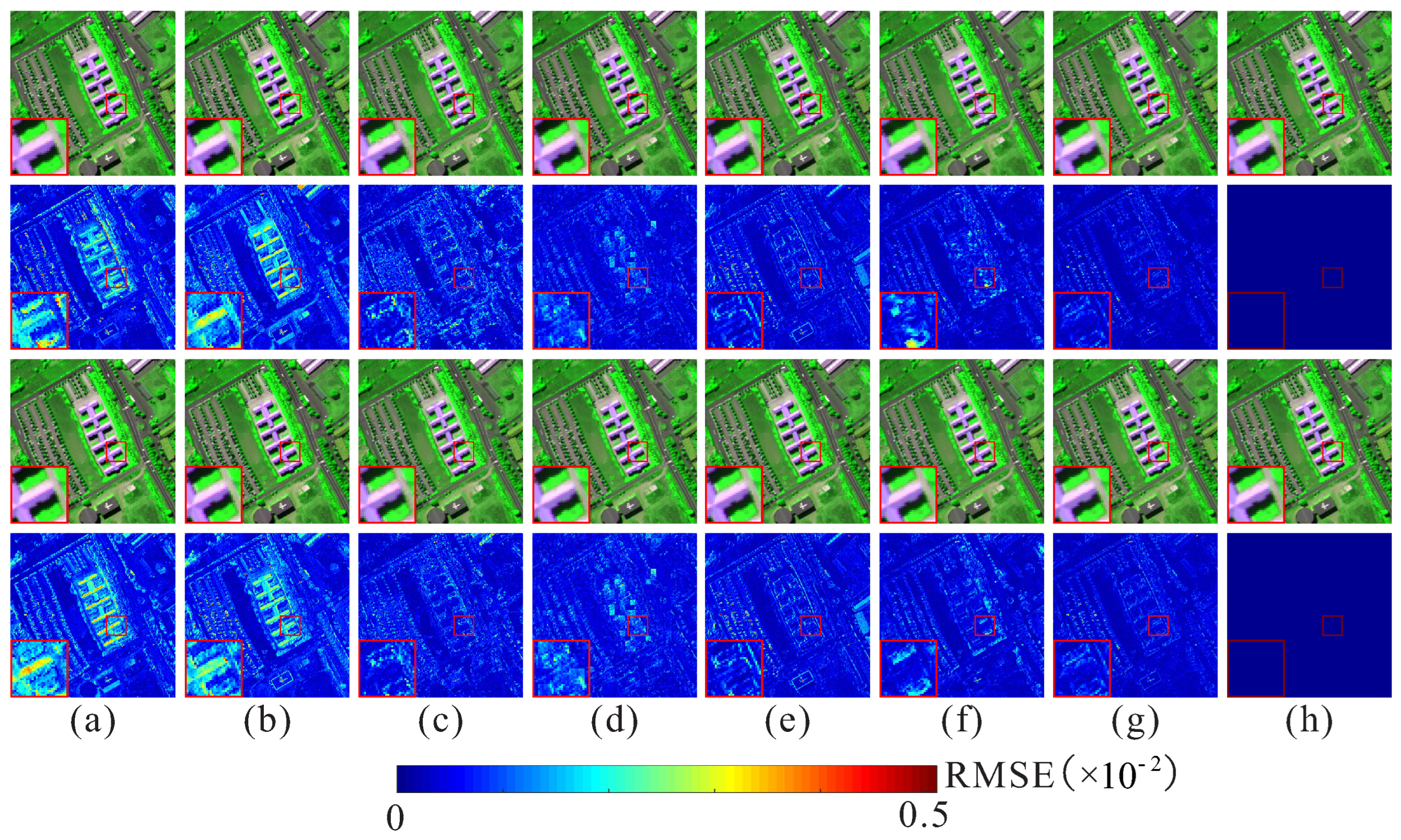
Figure 3 and Figure 4 demonstrate the fused results and their corresponding pixel-wise root mean square error (RMSE) images [61] of the simulated PU and WDCM datasets with uniform blur, respectively. The color images for the PU are generated using the 30th, 73rd, and 13th spectral bands. Similarly, the color images for the WDCM are created using the 75th, 45th, and 8th spectral bands. Meanwhile, we enlarge a specific region of interest (highlighted with a red block) to facilitate a more detailed visual comparison. Upon closer examination of the magnified regions, it becomes evident that all of the fused images display a notable improvement in spatial details. However, there are also noticeable spectral inconsistencies between the reference and fused images. For instance, we can see that the fused images of CNMF and HySure show noticeable spectral distortions in the building areas. Similarly, NSSR, GSFus, and LTMR produce a slight degree of spectral distortion in the tree areas. Additionally, the fused image of JSSLL1 clearly exhibits the presence of box effects on the PU dataset. Compared to other methods, our FGSSR-based method performs better in preserving spatial features and maintaining consistent spectral information.
To assess the spectral preservation capabilities of the test methods, the spectral curves of the fused results are compared in Figure 5. A clear observation from the comparison of spectral curves is that the fused results generated by the FGSSR-based method exhibit higher spectral consistency with the reference images across the majority of spectral bands. This finding suggests that the FGSSR-based method outperforms other compared methods in maintaining spectral accuracy. This can be attributed to the superior capability of the FGSSR model in capturing and preserving spectral correlation properties.
4.3.2. Results on Gaussian Blur Simulated Datasets
Meanwhile, we also verify the effectiveness of our FGSSR-based method in handling the simulated datasets generated by Gaussian blur. To obtain the LR-HSIs, we downsample every eight-pixel cluster along the spatial modes after applying an Gaussian blur (standard deviation 2.25) to the reference HR-HSIs obtained from the PU and WDCM datasets. The HR-MSIs are simulated by utilizing the IKONOS-like SRRF [60]. The results on the Gaussian blur simulated datasets are reported in Table 3. The optimal values are emphasized in bold to enhance understanding. From the table, matrix factorization-based methods have poor performance in Gaussian blur cases compared with tensor factorization-based methods. For example, the best-performing matrix factorization-based method NSSR achieved a SAM of 2.2543 on the Gaussian blur-simulated PU dataset, while the worst performing tensor factorization-based method JSSLL1 achieved a SAM of 2.1845. Table 3 also demonstrates that for both of the Gaussian blur simulated datasets, the FGSSR-based method outperforms the competition on the basis of all quality measures. This suggests that the FGSSR-based method exhibits superior performance in comparison to other SOTA methods in handling various blur functions and scaling factors.
4.3.3. Results on Noisy Simulated Datasets
In real-world scenarios, both HS and MS imaging processes typically introduce additive noise, with the noise level in the HR-MSI usually being lower than that in the LR-HSI. To evaluate the robustness of the FGSSR-based method under the influence of noise, we conducted tests using the noisy simulated datasets generated from the Chikusei dataset. Specifically, the noisy LR-HSI was simulated by adding Gaussian white noise after downsampling the reference Chikusei HSI using uniform averaging over blocks. For the noisy HR-MSI, it can be simulated by adding Gaussian white noise after filtering the reference Chikusei HR-HSI with an IKONOS-like SRRF. Specifically, the FGSSR-based method was verified in two different noisy cases:
Noisy case 1: SNRh = 35 dB, SNRm = 40 dB;
Noisy case 2: SNRh = 30 dB, SNRm = 35 dB,
where SNRh and SNRm represent the SNR of the noisy LR-HSI and HR-MSI, respectively.
Figure 6 shows the fused results and their corresponding RMSE images of the noisy cases on the Chikusei. The color images for the Chikusei were generated using the 60th, 39th, and 10th spectral bands. As seen in Figure 6, noise artefacts are presented in the fused results of CNMF, HySure, JSSLL1, GSFus, and LTMR. NSSR is sensitive to noise variations, and some noticeable block artifacts can be found in its fused images. The proposed FGSSR-based method achieved superior results with fewer errors compared to the other test methods. Table 4 reports the results on the noisy simulated datasets, further demonstrating that the FGSSR-based method performed better than other compared methods in dealing with noisy scenarios.
4.4. Experimental Results on Real Dataset
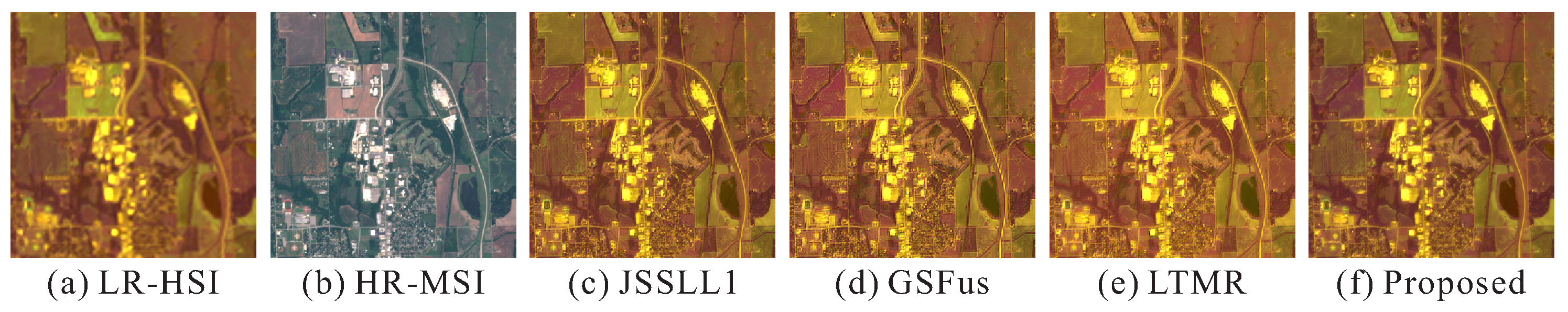
To verify the practical validity of the FGSSR-based method in real-life scenarios, we conducted an experiment using a real dataset. The details of this dataset can be found in Section 4.1. During the real experiment, we encountered the challenges of the unknown spectral response and the spatial downsampling method. To address these issues, we employed the method provided in [27] to calculate the unknown spectral response and spatial blur kernel. Figure 7 shows the fused results on the real dataset. From Figure 7, the fused images of JSSLL1 and GSFus exhibit aliasing effects in the road, implying that the preservation of spatial structures and details is not entirely satisfactory. Additionally, there are noticeable artificial effects and spectral distortions present in the LTMR results. The FGSSR-based method strikes a better balance between preserving spatial structures and minimizing spectral distortions than other methods, resulting in superior visual quality in its fused result. Figure 8 demonstrates the spectral curves of the fused images and the real LR-HSI. In Figure 8, we can see that the spectral curves of the compared methods are consistent with the spectral curve of the real LR-HSI, while the spectral curve of the fused result of the proposed FGSSR-based method exhibits the highest level of consistency with that of the real LR-HSI. This demonstrates the excellent performance of the FGSSR-based method in real-life scenarios, showcasing its practical effectiveness.
5. Discussion
In this part, the PU and WDCM datasets are selected as the experimental objects. The LR-HSIs are simulated by using an Gaussian blur function (Standard deviation 3) and a spatial Downsampling factor 8, and the HR-MSIs are generated by using an IKONOS-like SRRF. Additionally, Gaussian white noise is injected into the simulated LR-HSIs (SNRh = 35 dB) and HR-MSIs (SNRm = 40 dB).
5.1. The Effectiveness of the Proposed FGSSR Model
To demonstrate the effectiveness of the proposed Factor group sparsity regularized subspace representation (FGSSR) model (13), we carried out a comprehensive analysis by comparing our FGSSR-based fusion method with the fusion method based on the Direct subspace representation (DSR) model (12). By replacing the FGSSR model (13) with the DSR model (12), the DSR-based fusion method can be written as
In the experiments, the subspace dimension of the DSR-based fusion method was set to be consistent with the subspace dimension adaptively determined by the FGSSR-based fusion method. Table 5 presents the quantitative results of the FGSSR-based and DSR-based fusion methods on the simulated PU and WDCM datasets. From Table 5, it is evident that the FGSSR model (13) exhibited superior performance compared to the DSR model (12), delivering significantly better results on both of the two simulated datasets.
5.2. Analysis of Model Parameters
Parameter is utilized to constrain the spectral fidelity term. Figure 9a illustrates the PSNR curves corresponding to various values of . In Figure 9a, the PSNR values for the simulated PU and WDCM datasets remain relatively stable within the range of from to , but sharply decrease for greater than . This reveals that the proposed FGSSR-based method exhibits relatively robust performance for both of the two simulated datasets when . Therefore, is set for the proposed method in all experiments.
Parameter serves to restrict the spatial fidelity term. Figure 9b displays the PSNR curves corresponding to various values of . In the experiment, is varied within the range of . We can see from Figure 9b that there are obvious similarities between the trends of changes in the PSNR curves of two simulated datasets. This reveals that our FGSSR-based method is robust and stable across different datasets. The PSNR values for both the two simulated datasets experience a significant increase when varies from to , and then stabilize at the maximum level when varies from to . As a result, we assign a value of to the proposed FGSSR-based method in all conducted experiments.
To evaluate the impact of the parameter on the FGSSR-based method, experiments are conducted on the simulated PU and WDCM datasets using different values of . In the experiment, is selected from the set , . Figure 9c illustrates the PSNR curves for different . According to Figure 9c, the PSNR values for the simulated PU and WDCM datasets remain relatively stable within the range of from to , but decrease when exceeds . Based on these observations, is selected as the optimal value for the proposed method in all experiments.
Parameter w is utilized to constrain the TNN regularization term. To examine the effectiveness of the TNN regularization term, the proposed FGSSR-based method is applied to the simulated PU and WDCM datasets using varying values of w. Figure 9e illustrates the PSNR curves corresponding to various values of parameter w. According to Figure 9e, the PSNR values for both the simulated PU and WDCM datasets show increasing trends as w increases. This demonstrates that the TNN regularization applied to the low-dimensional coefficients enhances the ability of the proposed method in capturing spatial self-similarity features, ultimately leading to improved HR-HSI reconstruction. Additionally, the optimal outcomes for both of the two simulated datasets are attained when the value of w lies within the interval of . Taking this into consideration, is selected as the optimal value for the proposed method in all experiments.
is a proximal parameter that ensures the theoretical convergence of the PAM solver, while parameter serves as a penalty parameter. Figure 9f,g display the PSNR of the fused results for the simulated PU and WDCM datasets as functions of and , respectively. According to Figure 9f,g, the optimal results for both of the two simulated datasets are achieved when the value of is within the interval of , while the value of is within the range of . Based on these observations, and are set for the proposed method in all experiments.
5.3. Automatic Adjustment of Subspace Dimension
The proposed FGSSR-based method adaptively determines the subspace dimension by minimizing the number of nonzero frontal slices of coefficients during the iteration process. This adaptive strategy allows the FGSSR-based method dynamic adjustment of the subspace dimension to approximate the rank of the latent HR-HSI. Therefore, the FGSSR-based method can effectively capture the spectral correlation property and enhance the overall quality of the fused results. Figure 10 shows the variation of subspace dimension as the iteration increases. As shown in Figure 10, the subspace dimension exhibits a notable decline as the iteration progresses, ultimately reaching a state of convergence where it stabilises. Moreover, the convergence behavior of the subspace dimension differs between the simulated PU dataset and the simulated WDCM dataset. This emphasizes the significance of our proposed FGSSR-based method, which has the ability to dynamically identify the optimal subspace dimension, ensuring accurate and robust fused results across a wide range of datasets.
5.4. Computation Efficiency
Table 6 provides the calculation time in seconds for the test methods. All experiments were executed on a computer featuring a 1.7 GHz Intel Core i5-1240P CPU and 16 GB of RAM using MathWorks MATLAB R2016a. The primary components contributing to the computational complexity of Algorithm 3 are the and subproblems. For the subproblem, tensor product and TNN computations take up the majority of CPU time. The subproblem is a nonconvex sparse problem that can be efficiently addressed using the GST algorithm. From Table 6, it is evident that our FGSSR-based method consumes the least calculation time compared to other methods, despite the presence of inter and outer iterations in Algorithm 3.
5.5. Numerical Convergence
Figure 11 illustrates the variation in relative change (Rech), defined as , of the FGSSR-based method on the simulated PU and WDCM datasets as the iteration progresses. As shown in Figure 11, the Rech quickly converges to zero within a few iterations, demonstrating the fast and favorable numerical convergence of our FGSSR-based method.
6. Conclusions
In this study, we present a novel FGSSR-based method for HSI super-resolution. In our FGSSR-based method, the high spectral correlation property in HR-HSI is effectively modeled by the proposed FGSSR model, which offers several advantages, including enhanced rank minimization, adaptive subspace dimension determination, and low computational cost. Moreover, we employ TNN regularization on the low-dimensional coefficients to depict the spatial self-similarity property in HR-HSI, which offers high efficiency while effectively preserving the spatial features of HR-HSI. An efficient PAM-based algorithm is developed to solve the FGSSR-based model. The FGSSR-based method is evaluated against the SOTA HSI super-resolution methods using the simulated and real-world datasets. The comparison is conducted through visual and quantitative analysis, which reveals the superior performance of our FGSSR-based method.
Despite these promising results, there are several areas that require further investigation. For example, our proposed method currently concentrates solely on the global spatial self-similarity of HR-HSI, which aids in reducing computational complexity but may limit its ability to reconstruct spatial structure and preserve spatial details. Therefore, our future work will focus on employing the nonlocal self-similarity property of HR-HSI under the FGSSR framework to enhance the performance of HSI super-resolution. In addition, we plan to further extend our proposed method to a broader range of hyperspectral datasets for comparative analysis, aiming to provide a more comprehensive stability assessment of our proposed method. Furthermore, work [62] provides a novel sight to improve the quality of remote sensing images. Thus, our other future work is focused on enhancing the spatial resolution of HSI from the perspective of dynamic differential evolution theory.
Author Contributions
Conceptualization, Y.P. and W.L.; methodology, Y.P.; software, X.L.; validation, J.D., Y.P. and W.L.; formal analysis, Y.P.; investigation, Y.P.; resources, Y.P.; data curation, X.L.; writing—original draft preparation, Y.P.; writing—review and editing, W.L.; visualization, X.L.; supervision, J.D. All authors have read and agreed to the published version of the manuscript.
Funding
This research was funded by Special Funding for Postdoctoral Research Projects of Chongqing (Grant number 2022CQBSHTB3103), National Natural Science Foundation of China (Grant numbers 62331008, 61972060, 62027827,62176071) and National Key Research and Development Program of China (Grant number 2019YFE0110800).
Data Availability Statement
Data sharing is not applicable to this article.
Acknowledgments
The authors would like to thank all the reviewers for their valuable contributions to our work.
Conflicts of Interest
The authors declare no conflict of interest.
References
- Zhang, Z.; Ding, Y.; Zhao, X.; Siye, L.; Yang, N.; Cai, Y.; Zhan, Y. Multireceptive field: An adaptive path aggregation graph neural framework for hyperspectral image classification. Expert Syst. Appl. 2023, 217, 119508. [Google Scholar] [CrossRef]
- Ding, Y.; Zhang, Z.; Zhao, X.; Hong, D.; Li, W.; Cai, W.; Zhan, Y. AF2GNN: Graph convolution with adaptive filters and aggregator fusion for hyperspectral image classification. Inf. Sci. 2022, 602, 201–219. [Google Scholar] [CrossRef]
- Zhang, Y.; Kong, X.; Deng, L.; Liu, Y. Monitor water quality through retrieving water quality parameters from hyperspectral images using graph convolution network with superposition of multi-point effect: A case study in Maozhou River. J. Environ. Manag. 2023, 342, 118283. [Google Scholar] [CrossRef]
- Wang, L.; Wang, L.; Wang, Q.; Atkinson, P.M. SSA-SiamNet: Spectral–spatial-wise attention-based Siamese network for hyperspectral image change detection. IEEE Trans. Geosci. Remote Sens. 2021, 60, 1–18. [Google Scholar] [CrossRef]
- Liu, C.; Fan, Z.; Zhang, G. GJTD-LR: A Trainable Grouped Joint Tensor Dictionary With Low-Rank Prior for Single Hyperspectral Image Super-Resolution. IEEE Trans. Geosci. Remote Sens. 2022, 60, 1–17. [Google Scholar] [CrossRef]
- Xu, T.; Huang, T.Z.; Deng, L.J.; Yokoya, N. An iterative regularization method based on tensor subspace representation for hyperspectral image super-resolution. IEEE Trans. Geosci. Remote Sens. 2022, 60, 1–16. [Google Scholar]
- Ding, M.; Fu, X.; Huang, T.Z.; Wang, J.; Zhao, X.L. Hyperspectral super-resolution via interpretable block-term tensor modeling. IEEE J. Sel. Top. Signal Process. 2020, 15, 641–656. [Google Scholar] [CrossRef]
- Peng, Y.; Li, W.; Luo, X.; Du, J.; Gan, Y.; Gao, X. Integrated fusion framework based on semicoupled sparse tensor factorization for spatio-temporal–spectral fusion of remote sensing images. Inf. Fusion 2021, 65, 21–36. [Google Scholar] [CrossRef]
- Dian, R.; Li, S.; Fang, L. Learning a low tensor-train rank representation for hyperspectral image super-resolution. IEEE Trans. Neural Netw. Learn. Syst. 2019, 30, 2672–2683. [Google Scholar] [CrossRef]
- Li, Y.; Du, Z.; Wu, S.; Wang, Y.; Wang, Z.; Zhao, X.; Zhang, F. Progressive split-merge super resolution for hyperspectral imagery with group attention and gradient guidance. ISPRS J. Photogramm. Remote Sens. 2021, 182, 14–36. [Google Scholar] [CrossRef]
- Li, X.; Yuan, Y.; Wang, Q. Hyperspectral and multispectral image fusion via nonlocal low-rank tensor approximation and sparse representation. IEEE Trans. Geosci. Remote Sens. 2020, 59, 550–562. [Google Scholar] [CrossRef]
- Wu, X.; Huang, T.Z.; Deng, L.J.; Zhang, T.J. Dynamic cross feature fusion for remote sensing pansharpening. In Proceedings of the IEEE/CVF International Conference on Computer Vision, Montreal, BC, Canada, 11–17 October 2021; pp. 14687–14696. [Google Scholar]
- Cao, X.; Fu, X.; Hong, D.; Xu, Z.; Meng, D. PanCSC-Net: A model-driven deep unfolding method for pansharpening. IEEE Trans. Geosci. Remote Sens. 2021, 60, 1–13. [Google Scholar] [CrossRef]
- Hu, J.F.; Huang, T.Z.; Deng, L.J.; Jiang, T.X.; Vivone, G.; Chanussot, J. Hyperspectral image super-resolution via deep spatiospectral attention convolutional neural networks. IEEE Trans. Neural Netw. Learn. Syst. 2021, 33, 7251–7265. [Google Scholar] [CrossRef] [PubMed]
- Liu, J.; Wu, Z.; Xiao, L.; Wu, X.J. Model inspired autoencoder for unsupervised hyperspectral image super-resolution. IEEE Trans. Geosci. Remote Sens. 2022, 60, 1–12. [Google Scholar] [CrossRef]
- Fu, X.; Jia, S.; Xu, M.; Zhou, J.; Li, Q. Fusion of hyperspectral and multispectral images accounting for localized inter-image changes. IEEE Trans. Geosci. Remote Sens. 2021, 60, 1–18. [Google Scholar] [CrossRef]
- Xu, T.; Huang, T.Z.; Deng, L.J.; Zhao, X.L.; Huang, J. Hyperspectral image superresolution using unidirectional total variation with tucker decomposition. IEEE J. Sel. Top. Appl. Earth Obs. Remote Sens. 2020, 13, 4381–4398. [Google Scholar] [CrossRef]
- He, W.; Chen, Y.; Yokoya, N.; Li, C.; Zhao, Q. Hyperspectral super-resolution via coupled tensor ring factorization. Pattern Recognit. 2022, 122, 108280. [Google Scholar] [CrossRef]
- Chen, Y.; Zeng, J.; He, W.; Zhao, X.L.; Huang, T.Z. Hyperspectral and Multispectral Image Fusion Using Factor Smoothed Tensor Ring Decomposition. IEEE Trans. Geosci. Remote Sens. 2022, 60, 1–17. [Google Scholar] [CrossRef]
- Li, K.; Zhang, W.; Yu, D.; Tian, X. HyperNet: A deep network for hyperspectral, multispectral, and panchromatic image fusion. ISPRS J. Photogramm. Remote Sens. 2022, 188, 30–44. [Google Scholar] [CrossRef]
- Dian, R.; Li, S.; Guo, A.; Fang, L. Deep hyperspectral image sharpening. IEEE Trans. Neural Netw. Learn. Syst. 2018, 29, 5345–5355. [Google Scholar] [CrossRef]
- Qu, Y.; Qi, H.; Kwan, C. Unsupervised sparse dirichlet-net for hyperspectral image super-resolution. In Proceedings of the IEEE Conference on Computer Vision and Pattern Recognition, Salt Lake City, UT, USA, 18–22 June 2018; pp. 2511–2520. [Google Scholar]
- Zhang, L.; Nie, J.; Wei, W.; Zhang, Y.; Liao, S.; Shao, L. Unsupervised adaptation learning for hyperspectral imagery super-resolution. In Proceedings of the IEEE/CVF Conference on Computer Vision and Pattern Recognition, Seattle, WA, USA, 14–19 June 2020; pp. 3073–3082. [Google Scholar]
- Wycoff, E.; Chan, T.H.; Jia, K.; Ma, W.K.; Ma, Y. A non-negative sparse promoting algorithm for high resolution hyperspectral imaging. In Proceedings of the IEEE International Conference on Acoustics, Speech and Signal Processing, Vancouver, BC, Canada, 26–31 May 2013; pp. 1409–1413. [Google Scholar]
- Lanaras, C.; Baltsavias, E.; Schindler, K. Hyperspectral super-resolution by coupled spectral unmixing. In Proceedings of the IEEE International Conference on Computer Vision, Santiago, Chile, 7–13 December 2015; pp. 3586–3594. [Google Scholar]
- Xue, J.; Zhao, Y.Q.; Bu, Y.; Liao, W.; Chan, J.C.W.; Philips, W. Spatial-spectral structured sparse low-rank representation for hyperspectral image super-resolution. IEEE Trans. Image Process. 2021, 30, 3084–3097. [Google Scholar] [CrossRef] [PubMed]
- Simoes, M.; Bioucas-Dias, J.; Almeida, L.B.; Chanussot, J. A convex formulation for hyperspectral image superresolution via subspace-based regularization. IEEE Trans. Geosci. Remote Sens. 2014, 53, 3373–3388. [Google Scholar] [CrossRef]
- Dong, W.; Fu, F.; Shi, G.; Cao, X.; Wu, J.; Li, G.; Li, X. Hyperspectral image super-resolution via non-negative structured sparse representation. IEEE Trans. Image Process. 2016, 25, 2337–2352. [Google Scholar] [CrossRef] [PubMed]
- Zhang, K.; Wang, M.; Yang, S.; Jiao, L. Spatial–spectral-graph-regularized low-rank tensor decomposition for multispectral and hyperspectral image fusion. IEEE J. Sel. Top. Appl. Earth Obs. Remote Sens. 2018, 11, 1030–1040. [Google Scholar] [CrossRef]
- Li, S.; Dian, R.; Fang, L.; Bioucas-Dias, J.M. Fusing hyperspectral and multispectral images via coupled sparse tensor factorization. IEEE Trans. Image Process. 2018, 27, 4118–4130. [Google Scholar] [CrossRef]
- Xu, Y.; Wu, Z.; Chanussot, J.; Wei, Z. Hyperspectral images super-resolution via learning high-order coupled tensor ring representation. IEEE Trans. Neural Netw. Learn. Syst. 2020, 31, 4747–4760. [Google Scholar] [CrossRef]
- Kanatsoulis, C.I.; Fu, X.; Sidiropoulos, N.D.; Ma, W.K. Hyperspectral super-resolution: A coupled tensor factorization approach. IEEE Trans. Signal Process. 2018, 66, 6503–6517. [Google Scholar] [CrossRef]
- Xu, Y.; Wu, Z.; Chanussot, J.; Wei, Z. Nonlocal patch tensor sparse representation for hyperspectral image super-resolution. IEEE Trans. Image Process. 2019, 28, 3034–3047. [Google Scholar] [CrossRef]
- Xue, J.; Zhao, Y.; Huang, S.; Liao, W.; Chan, J.C.W.; Kong, S.G. Multilayer sparsity-based tensor decomposition for low-rank tensor completion. IEEE Trans. Neural Netw. Learn. Syst. 2021, 33, 6916–6930. [Google Scholar] [CrossRef]
- Dian, R.; Fang, L.; Li, S. Hyperspectral image super-resolution via non-local sparse tensor factorization. In Proceedings of the IEEE Conference on Computer Vision and Pattern Recognition, Dhaka, Bangladesh, 13–14 February 2017; pp. 5344–5353. [Google Scholar]
- Borsoi, R.A.; Prévost, C.; Usevich, K.; Brie, D.; Bermudez, J.C.; Richard, C. Coupled tensor decomposition for hyperspectral and multispectral image fusion with inter-image variability. IEEE J. Sel. Top. Signal Process. 2021, 15, 702–717. [Google Scholar] [CrossRef]
- Han, H.; Liu, H. Hyperspectral image super-resolution based on transform domain low rank tensor regularization. In Proceedings of the 2022 International Conference on Image Processing and Media Computing (ICIPMC), Xi’an, China, 27–29 May 2022; pp. 80–84. [Google Scholar]
- Dian, R.; Li, S. Hyperspectral Image Super-Resolution via Subspace-Based Low Tensor Multi-Rank Regularization. IEEE Trans. Image Process. 2019, 28, 5135–5146. [Google Scholar] [CrossRef] [PubMed]
- Xing, Y.; Zhang, Y.; Yang, S.; Zhang, Y. Hyperspectral and multispectral image fusion via variational tensor subspace decomposition. IEEE Geosci. Remote Sens. Lett. 2021, 19, 1–5. [Google Scholar] [CrossRef]
- Xu, H.; Qin, M.; Chen, S.; Zheng, Y.; Zheng, J. Hyperspectral-multispectral image fusion via tensor ring and subspace decompositions. IEEE J. Sel. Top. Appl. Earth Obs. Remote Sens. 2021, 14, 8823–8837. [Google Scholar] [CrossRef]
- Xue, S.; Qiu, W.; Liu, F.; Jin, X. Low-rank tensor completion by truncated nuclear norm regularization. In Proceedings of the 24th International Conference on Pattern Recognition (ICPR), Beijing, China, 20–24 August 2018; pp. 2600–2605. [Google Scholar]
- Kilmer, M.E.; Braman, K.; Hao, N.; Hoover, R.C. Third-order tensors as operators on matrices: A theoretical and computational framework with applications in imaging. SIAM J. Matrix Anal. Appl. 2013, 34, 148–172. [Google Scholar] [CrossRef]
- Lu, C.; Feng, J.; Chen, Y.; Liu, W.; Lin, Z.; Yan, S. Tensor robust principal component analysis with a new tensor nuclear norm. IEEE Trans. Pattern Anal. Mach. Intell. 2019, 42, 925–938. [Google Scholar] [CrossRef] [PubMed]
- Nie, F.; Huang, H.; Ding, C. Low-rank matrix recovery via efficient schatten p-norm minimization. In Proceedings of the AAAI Conference on Artificial Intelligence, Toronto, ON, Canada, 22–26 July 2012; Volume 26, pp. 655–661. [Google Scholar]
- Fan, J.; Ding, L.; Chen, Y.; Udell, M. Factor group-sparse regularization for efficient low-rank matrix recovery. Adv. Neural Inf. Process. Syst. 2019, 32, 5105–5115. [Google Scholar]
- Fang, L.; Zhuo, H.; Li, S. Super-resolution of hyperspectral image via superpixel-based sparse representation. Neurocomputing 2018, 273, 171–177. [Google Scholar] [CrossRef]
- Zhao, C.; Gao, X.; Emery, W.J.; Wang, Y.; Li, J. An Integrated Spatio-Spectral–Temporal Sparse Representation Method for Fusing Remote-Sensing Images With Different Resolutions. IEEE Trans. Geosci. Remote Sens. 2018, 56, 3358–3370. [Google Scholar] [CrossRef]
- Peng, Y.; Li, W.; Luo, X.; Du, J. Hyperspectral image superresolution using global gradient sparse and nonlocal low-rank tensor decomposition with hyper-laplacian prior. IEEE J. Sel. Top. Appl. Earth Obs. Remote Sens. 2021, 14, 5453–5469. [Google Scholar] [CrossRef]
- Li, X.; Huang, J.; Deng, L.J.; Huang, T.Z. Bilateral filter based total variation regularization for sparse hyperspectral image unmixing. Inf. Sci. 2019, 504, 334–353. [Google Scholar] [CrossRef]
- Chen, Y.; Huang, T.Z.; He, W.; Zhao, X.L.; Zhang, H.; Zeng, J. Hyperspectral image denoising using factor group sparsity-regularized nonconvex low-rank approximation. IEEE Trans. Geosci. Remote Sens. 2021, 60, 1–16. [Google Scholar] [CrossRef]
- Attouch, H.; Bolte, J.; Svaiter, B.F. Convergence of descent methods for semi-algebraic and tame problems: Proximal algorithms, forward–backward splitting, and regularized Gauss–Seidel methods. Math. Program. 2013, 137, 91–129. [Google Scholar] [CrossRef]
- Boyd, S.; Parikh, N.; Chu, E.; Peleato, B.; Eckstein, J. Distributed optimization and statistical learning via the alternating direction method of multipliers. Found. Trends® Mach. Learn. 2011, 3, 1–122. [Google Scholar]
- Zuo, W.; Meng, D.; Zhang, L.; Feng, X.; Zhang, D. A generalized iterated shrinkage algorithm for non-convex sparse coding. In Proceedings of the IEEE International Conference on Computer Vision, Manchester, UK, 13–16 October 2013; pp. 217–224. [Google Scholar]
- Yokoya, N.; Yairi, T.; Iwasaki, A. Coupled nonnegative matrix factorization unmixing for hyperspectral and multispectral data fusion. IEEE Trans. Geosci. Remote Sens. 2011, 50, 528–537. [Google Scholar] [CrossRef]
- Guo, H.; Bao, W.; Feng, W.; Sun, S.; Mo, C.; Qu, K. Multispectral and Hyperspectral Image Fusion Based on Joint-Structured Sparse Block-Term Tensor Decomposition. Remote Sens. 2023, 15, 4610. [Google Scholar] [CrossRef]
- Wald, L. Quality of high resolution synthesised images: Is there a simple criterion? In Proceedings of the Third Conference “Fusion of Earth Data: Merging Point Measurements, Raster Maps and Remotely Sensed Images”, Sophia Antipolis, France, 26–28 January 2000; pp. 99–103. [Google Scholar]
- Wang, Z.; Bovik, A.C.; Sheikh, H.R.; Simoncelli, E.P. Image quality assessment: From error visibility to structural similarity. IEEE Trans. Image Process. 2004, 13, 600–612. [Google Scholar] [CrossRef]
- Yuhas, R.H.; Goetz, A.F.; Boardman, J.W. Discrimination among semi-arid landscape endmembers using the spectral angle mapper (SAM) algorithm. In Proceedings of the Summaries 4th JPL Airborne Earth Sci. Workshop, Pasadena, CA, USA, 1–5 June 1992; pp. 147–149. [Google Scholar]
- Wang, Z.; Bovik, A.C. A universal image quality index. IEEE Signal Process. Lett. 2002, 9, 81–84. [Google Scholar] [CrossRef]
- Wei, Q.; Bioucas-Dias, J.; Dobigeon, N.; Tourneret, J.Y. Hyperspectral and multispectral image fusion based on a sparse representation. IEEE Trans. Geosci. Remote Sens. 2015, 53, 3658–3668. [Google Scholar] [CrossRef]
- Yokoya, N.; Grohnfeldt, C.; Chanussot, J. Hyperspectral and multispectral data fusion: A comparative review of the recent literature. IEEE Geosci. Remote Sens. Mag. 2017, 5, 29–56. [Google Scholar] [CrossRef]
- Singh, D.; Kaur, M.; Jabarulla, M.Y.; Kumar, V.; Lee, H.N. Evolving fusion-based visibility restoration model for hazy remote sensing images using dynamic differential evolution. IEEE Trans. Geosci. Remote Sens. 2022, 60, 1–14. [Google Scholar] [CrossRef]
Figure 1.
Flowchart of the proposed fusion method. Note: Since the subspace is obtained using the subspace learning strategy from LR-HSI, the objective function no longer includes separate terms related to . The appearance of in this flowchart is intended to facilitate understanding.
Figure 1.
Flowchart of the proposed fusion method. Note: Since the subspace is obtained using the subspace learning strategy from LR-HSI, the objective function no longer includes separate terms related to . The appearance of in this flowchart is intended to facilitate understanding.

Figure 2.
FGSSR of the HR-HSI.

Figure 3.
Fused and RMSE images of the simulated PU dataset with uniform blur and scaling factor (1st and 2nd rows) and (3rd and 4th rows). (a) CNMF. (b) HySure. (c) NSSR. (d) JSSLL1. (e) GSFus. (f) LTMR. (g) Proposed method. (h) Reference image.
Figure 3.
Fused and RMSE images of the simulated PU dataset with uniform blur and scaling factor (1st and 2nd rows) and (3rd and 4th rows). (a) CNMF. (b) HySure. (c) NSSR. (d) JSSLL1. (e) GSFus. (f) LTMR. (g) Proposed method. (h) Reference image.

Figure 4.
Fused and RMSE images of the simulated WDCM dataset with uniform blur and scaling factor (1st and 2nd rows) and (3rd and 4th rows). (a) CNMF. (b) HySure. (c) NSSR. (d) JSSLL1. (e) GSFus. (f) LTMR. (g) Proposed method. (h) Reference image.
Figure 4.
Fused and RMSE images of the simulated WDCM dataset with uniform blur and scaling factor (1st and 2nd rows) and (3rd and 4th rows). (a) CNMF. (b) HySure. (c) NSSR. (d) JSSLL1. (e) GSFus. (f) LTMR. (g) Proposed method. (h) Reference image.

Figure 5.
Spectral curves of the fused results for the uniform blur simulated datasets with . (a) Spectral curves of the pixel located at position (20, 136) in the fused PU HSI. (b) Spectral curves of the pixel located at position (120, 24) in the fused WDCM HSI.
Figure 5.
Spectral curves of the fused results for the uniform blur simulated datasets with . (a) Spectral curves of the pixel located at position (20, 136) in the fused PU HSI. (b) Spectral curves of the pixel located at position (120, 24) in the fused WDCM HSI.

Figure 6.
Fused and RMSE images of Noisy case 1 (1st and 2nd rows) and Noisy case 2 (3rd and 4th rows). (a) CNMF. (b) HySure. (c) NSSR. (d) JSSLL1. (e) GSFus. (f) LTMR. (g) Proposed method. (h) Reference image.
Figure 6.
Fused and RMSE images of Noisy case 1 (1st and 2nd rows) and Noisy case 2 (3rd and 4th rows). (a) CNMF. (b) HySure. (c) NSSR. (d) JSSLL1. (e) GSFus. (f) LTMR. (g) Proposed method. (h) Reference image.

Figure 7.
Fused results of the real dataset. (a) LR-HSI. (b) HR-MSI. (c) JSSLL1. (d) GSFus. (e) LTMR. (f) Proposed method.
Figure 7.
Fused results of the real dataset. (a) LR-HSI. (b) HR-MSI. (c) JSSLL1. (d) GSFus. (e) LTMR. (f) Proposed method.

Figure 8.
Spectral curves of the pixel located at position (20, 96) in the fused results and the pixel located at position (3, 32) in the real LR-HSI.
Figure 8.
Spectral curves of the pixel located at position (20, 96) in the fused results and the pixel located at position (3, 32) in the real LR-HSI.

Figure 9.
Sensitivity study on parameters (a) , (b) , (c) , (e) w, (f) , (g) .

Figure 10.
Variation of the subspace dimension d as the iteration increases. (a) The simulated PU dataset, and (b) the simulated WDCM dataset.
Figure 10.
Variation of the subspace dimension d as the iteration increases. (a) The simulated PU dataset, and (b) the simulated WDCM dataset.

Figure 11.
Rech variation as the iteration progresses of FGSSR-based method on (a) the simulated PU dataset and (b) the simulated WDCM dataset.
Figure 11.
Rech variation as the iteration progresses of FGSSR-based method on (a) the simulated PU dataset and (b) the simulated WDCM dataset.


Table 1.
Quantitative results on simulated PU dataset with uniform blur.
| Evaluation Index | PSNR | SAM | ERGAS | UIQI | SSIM |
|---|---|---|---|---|---|
| Best Value | 0 | 0 | 1 | 1 | |
| CNMF [54] | 42.107 | 1.9039 | 1.1855 | 0.9945 | 0.9896 |
| HySure [27] | 41.635 | 2.0066 | 1.2248 | 0.9940 | 0.9888 |
| NSSR [28] | 43.131 | 2.2042 | 1.1417 | 0.9921 | 0.9825 |
| JSSLL1 [55] | 44.022 | 1.8815 | 1.0145 | 0.9938 | 0.9896 |
| GSFus [16] | 43.697 | 2.0110 | 1.0409 | 0.9937 | 0.9891 |
| LTMR [38] | 44.953 | 1.6761 | 0.8867 | 0.9955 | 0.9912 |
| Proposed | 45.910 | 1.5669 | 0.7898 | 0.9963 | 0.9923 |
| CNMF [54] | 39.692 | 2.3796 | 0.7644 | 0.9907 | 0.9848 |
| HySure [27] | 39.087 | 2.5558 | 0.8246 | 0.9909 | 0.9841 |
| NSSR [28] | 42.757 | 2.3663 | 0.5939 | 0.9915 | 0.9820 |
| JSSLL1 [55] | 43.381 | 1.9963 | 0.5114 | 0.9935 | 0.9863 |
| GSFus [16] | 43.357 | 2.0910 | 0.5396 | 0.9933 | 0.9883 |
| LTMR [38] | 44.342 | 2.0232 | 0.5004 | 0.9946 | 0.9895 |
| Proposed | 45.101 | 1.7139 | 0.4357 | 0.9956 | 0.9913 |
| CNMF [54] | 39.161 | 2.4714 | 0.4103 | 0.9904 | 0.9844 |
| HySure [27] | 38.909 | 2.8017 | 0.4162 | 0.9893 | 0.9814 |
| NSSR [28] | 42.507 | 2.4716 | 0.3109 | 0.9911 | 0.9813 |
| JSSLL1 [55] | 42.737 | 2.2773 | 0.2920 | 0.9927 | 0.9862 |
| GSFus [16] | 43.253 | 2.1154 | 0.2732 | 0.9932 | 0.9880 |
| LTMR [38] | 43.979 | 2.1211 | 0.2522 | 0.9937 | 0.9889 |
| Proposed | 44.555 | 1.8265 | 0.2334 | 0.9950 | 0.9907 |
Table 2.
Quantitative results on simulated WDCM dataset with uniform blur.
| Evaluation Index | PSNR | SAM | ERGAS | UIQI | SSIM |
|---|---|---|---|---|---|
| Best Value | 0 | 0 | 1 | 1 | |
| CNMF [54] | 40.486 | 2.0643 | 1.2656 | 0.9927 | 0.9890 |
| HySure [27] | 40.731 | 2.2544 | 1.2953 | 0.9925 | 0.9865 |
| NSSR [28] | 41.151 | 2.3756 | 1.3732 | 0.9929 | 0.9821 |
| JSSLL1 [55] | 41.886 | 2.2584 | 1.2521 | 0.9933 | 0.9858 |
| GSFus [16] | 41.815 | 2.3285 | 1.3101 | 0.9923 | 0.9867 |
| LTMR [38] | 43.110 | 2.0396 | 1.1182 | 0.9949 | 0.9884 |
| Proposed | 43.752 | 1.6558 | 1.0408 | 0.9959 | 0.9914 |
| CNMF [54] | 39.452 | 2.4361 | 0.7205 | 0.9903 | 0.9863 |
| HySure [27] | 38.929 | 2.8177 | 0.8370 | 0.9887 | 0.9828 |
| NSSR [28] | 40.777 | 2.6519 | 0.7233 | 0.9903 | 0.9817 |
| JSSLL1 [55] | 41.068 | 2.594 | 0.7187 | 0.9918 | 0.9842 |
| GSFus [16] | 40.644 | 2.8770 | 0.7554 | 0.9899 | 0.9860 |
| LTMR [38] | 41.919 | 2.5506 | 0.7215 | 0.9924 | 0.9837 |
| Proposed | 42.452 | 2.0956 | 0.6218 | 0.9938 | 0.9886 |
| CNMF [54] | 37.418 | 3.1868 | 0.4567 | 0.9850 | 0.9823 |
| HySure [27] | 36.335 | 3.4996 | 0.5335 | 0.9816 | 0.9760 |
| NSSR [28] | 39.522 | 3.2146 | 0.4298 | 0.9869 | 0.9779 |
| JSSLL1 [55] | 39.809 | 2.8308 | 0.4135 | 0.9870 | 0.9789 |
| GSFus [16] | 38.449 | 3.3989 | 0.5049 | 0.9818 | 0.9799 |
| LTMR [38] | 40.335 | 2.8135 | 0.4611 | 0.9881 | 0.9793 |
| Proposed | 41.499 | 2.4277 | 0.3539 | 0.9917 | 0.9870 |
Table 3.
Quantitative results on simulated PU and WDCM datasets with Gaussian blur and q = 8.
| Evaluation Index | PSNR | SAM | ERGAS | UIQI | SSIM |
|---|---|---|---|---|---|
| Best Value | 0 | 0 | 1 | 1 | |
| PU dataset | |||||
| CNMF [54] | 39.144 | 2.3847 | 0.8216 | 0.9906 | 0.9847 |
| HySure [27] | 38.679 | 2.6830 | 0.8640 | 0.9901 | 0.9827 |
| NSSR [28] | 42.079 | 2.2543 | 0.6734 | 0.9914 | 0.9852 |
| JSSLL1 [55] | 42.851 | 2.1845 | 0.5923 | 0.9921 | 0.9863 |
| GSFus [16] | 43.195 | 2.1028 | 0.5467 | 0.9934 | 0.9884 |
| LTMR [38] | 44.125 | 1.9953 | 0.4924 | 0.9942 | 0.9893 |
| Proposed | 44.727 | 1.8090 | 0.4567 | 0.9953 | 0.9910 |
| WDCM dataset | |||||
| CNMF [54] | 38.932 | 2.5809 | 0.7642 | 0.9892 | 0.9848 |
| HySure [27] | 38.845 | 2.8448 | 0.8451 | 0.9885 | 0.9825 |
| NSSR [28] | 40.426 | 2.6366 | 0.7965 | 0.9899 | 0.9818 |
| JSSLL1 [55] | 40.543 | 2.5385 | 0.7145 | 0.9912 | 0.9834 |
| GSFus [16] | 40.804 | 2.5341 | 0.7234 | 0.9905 | 0.9864 |
| LTMR [38] | 41.225 | 2.6241 | 0.7939 | 0.9912 | 0.9809 |
| Proposed | 42.052 | 2.2358 | 0.6584 | 0.9931 | 0.9879 |
Table 4.
Quantitative results on the noisy simulated datasets of the Chikusei.
| Evaluation Index | PSNR | SAM | ERGAS | UIQI | SSIM |
|---|---|---|---|---|---|
| Best Value | 0 | 0 | 1 | 1 | |
| Noisy case 1 | |||||
| CNMF [54] | 41.192 | 1.4237 | 1.6872 | 0.9692 | 0.9855 |
| HySure [27] | 40.635 | 1.7182 | 1.8944 | 0.9631 | 0.9796 |
| NSSR [28] | 42.736 | 1.6560 | 1.5704 | 0.9644 | 0.9815 |
| JSSLL1 [55] | 43.365 | 1.4429 | 1.7172 | 0.9665 | 0.9828 |
| GSFus [16] | 43.723 | 1.4587 | 1.5946 | 0.9668 | 0.9861 |
| LTMR [38] | 44.517 | 1.3465 | 1.5730 | 0.9736 | 0.9867 |
| Proposed | 45.489 | 1.1652 | 1.4243 | 0.9742 | 0.9883 |
| Noisy case 2 | |||||
| CNMF [54] | 39.414 | 1.6403 | 1.7888 | 0.9623 | 0.9787 |
| HySure [27] | 39.596 | 2.0064 | 2.1211 | 0.9509 | 0.9678 |
| NSSR [28] | 39.450 | 2.4438 | 1.9339 | 0.9401 | 0.9624 |
| JSSLL1 [55] | 41.176 | 1.6936 | 1.9087 | 0.9584 | 0.9734 |
| GSFus [16] | 41.947 | 1.8207 | 1.6702 | 0.9581 | 0.9775 |
| LTMR [38] | 42.294 | 1.6918 | 1.7407 | 0.9610 | 0.9756 |
| Proposed | 43.295 | 1.4812 | 1.6072 | 0.9635 | 0.9794 |
Table 5.
Quantitative results of the FGSSR-based and DSR-based methods on the simulated PU and WDCM datasets.
Table 5.
Quantitative results of the FGSSR-based and DSR-based methods on the simulated PU and WDCM datasets.
| Methods | PU Dataset | WDCM Dataset | ||||||||
|---|---|---|---|---|---|---|---|---|---|---|
| PSNR | SAM | ERGAS | UIQI | SSIM | PSNR | SAM | ERGAS | UIQI | SSIM | |
| Best Value | 0 | 0 | 1 | 1 | 0 | 0 | 1 | 1 | ||
| DSR-based | 42.380 | 2.2899 | 0.5761 | 0.9923 | 0.9833 | 38.677 | 3.2126 | 0.8330 | 0.9821 | 0.9692 |
| FGSSR-based | 43.764 | 1.9899 | 0.4991 | 0.9942 | 0.9884 | 41.001 | 2.5193 | 0.7023 | 0.9911 | 0.9848 |
Table 6.
Calculation time of test methods on simulated datasets (in seconds).
| Dataset | CNMF | HySure | NSSR | JSSLL1 | GSFus | LTMR | Proposed |
|---|---|---|---|---|---|---|---|
| PU | 28.87 | 88.87 | 142.29 | 174.68 | 236.47 | 155.87 | 24.35 |
| WDCM | 37.14 | 94.40 | 145.68 | 211.45 | 243.33 | 160.92 | 25.84 |
Disclaimer/Publisher’s Note: The statements, opinions and data contained in all publications are solely those of the individual author(s) and contributor(s) and not of MDPI and/or the editor(s). MDPI and/or the editor(s) disclaim responsibility for any injury to people or property resulting from any ideas, methods, instructions or products referred to in the content. |
© 2023 by the authors. Licensee MDPI, Basel, Switzerland. This article is an open access article distributed under the terms and conditions of the Creative Commons Attribution (CC BY) license (https://creativecommons.org/licenses/by/4.0/).
Share and Cite
MDPI and ACS Style
Peng, Y.; Li, W.; Luo, X.; Du, J. Hyperspectral Image Super-Resolution via Adaptive Factor Group Sparsity Regularization-Based Subspace Representation. Remote Sens. 2023, 15, 4847. https://0-doi-org.brum.beds.ac.uk/10.3390/rs15194847
AMA Style
Peng Y, Li W, Luo X, Du J. Hyperspectral Image Super-Resolution via Adaptive Factor Group Sparsity Regularization-Based Subspace Representation. Remote Sensing. 2023; 15(19):4847. https://0-doi-org.brum.beds.ac.uk/10.3390/rs15194847
Chicago/Turabian StylePeng, Yidong, Weisheng Li, Xiaobo Luo, and Jiao Du. 2023. "Hyperspectral Image Super-Resolution via Adaptive Factor Group Sparsity Regularization-Based Subspace Representation" Remote Sensing 15, no. 19: 4847. https://0-doi-org.brum.beds.ac.uk/10.3390/rs15194847
Note that from the first issue of 2016, this journal uses article numbers instead of page numbers. See further details here.