Article

Enhanced Point Cloud Slicing Method for Volume Calculation of Large Irregular Bodies: Validation in Open-Pit Mining

1
School of Remote Sensing and Information Engineering, Wuhan University, Wuhan 430072, China
2
Hubei Luojia Laboratory, Wuhan 430072, China
3
School of Mining and Geomatics Engineering, Hebei University of Engineering, Handan 056038, China
4
Research Center of Hebei Province Ecological Civilization and Social Governance, Hebei University of Engineering, Handan 056038, China
5
Guangxi Taiwei Information Technology Co., Ltd., Guilin 541000, China
6
Lands and Resource Department of Guangdong Province, Surveying and Mapping Institute, Guangzhou 510500, China
*
Author to whom correspondence should be addressed.
These authors contributed equally to this work.
Remote Sens. 2023, 15(20), 5006; https://0-doi-org.brum.beds.ac.uk/10.3390/rs15205006
Submission received: 2 August 2023 / Revised: 13 September 2023 / Accepted: 8 October 2023 / Published: 18 October 2023
(This article belongs to the Special Issue New Perspectives on 3D Point Cloud II)

Abstract

:
The calculation of volumes for irregular bodies holds significant relevance across various production processes. This spans tasks such as evaluating the growth status of crops and fruits, conducting morphological analyses of spatial objects based on volume parameters, and estimating quantities for earthwork and excavation. While methods like drainage, surface reconstruction, and triangulation suffice for smaller irregular bodies, larger ones introduce heightened complexity. Technological advancements, such as UAV photogrammetry and LiDAR, have introduced efficient point cloud data acquisition methods, bolstering precision and efficiency in calculating volumes for substantial irregular bodies. Notably, open-pit mines, characterized by their dynamic surface alterations, exemplify the challenges posed by large irregular bodies. Ensuring accurate excavation quantity calculations in such mines is pivotal, impacting operational considerations, acceptance, as well as production cost management and project oversight. Thus, this study employs UAV-acquired point cloud data from open-pit mines as a case study. In practice, calculating volumes for substantial irregular bodies often relies on the point cloud slicing method. However, this approach grapples with distinguishing multi-contour boundaries, leading to inaccuracies. To surmount this hurdle, this paper introduces an enhanced point cloud slicing method. The methodology involves segmenting point cloud data at fixed intervals, followed by the segmentation of slice contours using the Euclidean clustering method. Subsequently, the concave hull algorithm extracts the contour polygons of each slice. The final volume calculation involves multiplying the area of each polygon by the spacing and aggregating these products. To validate the efficacy of our approach, we employ model-derived volumes as benchmarks, comparing errors arising from both the traditional slicing method and our proposed technique. Experimental outcomes underscore the superiority of our point cloud volume calculation method, manifesting in an average relative error of 1.17%, outperforming the conventional point cloud slicing method in terms of accuracy.

1. Introduction

The calculation of irregular volumes is a common practice in various production processes. For smaller irregular volumes, precise calculations can be achieved using methods such as drainage. However, in scenarios where there is a need to accurately model irregular bodies while preserving fine texture information, often at the cost of computational efficiency, techniques like voxelization are commonly employed, particularly in fields like gaming and the medical sector [1,2]. Nevertheless, these methods are still not well suited for efficiently calculating the volume of larger irregular bodies. In this paper, we elucidate the challenges associated with calculating the volume of large irregular bodies, using the example of calculating excavation quantities in open-pit mining. Accurate excavation quantity calculation is pivotal for enhancing mine production monitoring and cost management, representing a fundamental task in open-pit mine surveying and acceptance [3]. In recent years, advanced methods with high accuracy and speed, such as 3D laser scanning and UAV photogrammetry, have been extensively employed for measuring excavation or settlement volumes [4,5,6], landslide analysis [7], and calculating mining volume [8]. These methods facilitate the rapid construction of 3D point cloud models for large-scale irregular bodies, such as open-pit mines [9]. The calculation of volume for large irregular bodies is typically achieved using specific methods. Some researchers have employed a combination of the Digital Elevation Model (DEM) with the grid method to calculate excavation volumes in open-pit mines [10]. However, this approach relies on DEM, which requires interpolating the point cloud into a grid during volume calculation. The non-continuous and non-differentiable surface characteristics of large irregular bodies can introduce errors in surface modeling using DEM, leading to deviations in the calculated volume [11,12].
Point cloud data provide denser sampling and better fitting properties, making them a more suitable choice than DEM for volume calculations. This substitution can significantly enhance calculation accuracy. Currently, methods for calculating the volume of irregular bodies using point cloud data can be broadly categorized into the inverse modeling method and the point cloud slicing method [13]. The inverse modeling method offers high accuracy in volume calculation but involves the complex construction of point cloud triangular meshes, often requiring cavity filling. Additionally, this method is computationally intensive in terms of time and space complexity [14,15,16]. In contrast, the point cloud slicing method utilizes the principles of calculus to divide the point cloud model into numerous micro-elements. It calculates the volume of the entire point cloud model by summing up the volumes of each individual micro-element. This approach allows for precise control of volume calculation accuracy [17,18]. Numerous researchers have conducted studies on this method. For instance, Hua et al. [19] proposed an improved volume calculation method based on the slicing approach. They employed the Alpha shape algorithm to construct the concave hull contour of the sliced point cloud, facilitating the measurement of rice seed volume. Zhi et al. [20] introduced a 3D point cloud volume calculation method based on the slicing approach. This method involves cutting the point cloud along the Z-axis projection coordinate system and projecting the point cloud data onto the XOY plane for volume calculation based on the projected area and slice distance. However, the accuracy of this method is significantly affected by the spacing between slices. Chang et al. [21] improved upon the traditional slicing method by implementing cuts along multiple coordinate axes and fitting the resulting slices to two curve functions. They then integrated these curves to estimate the area of each slice and calculate the volume of the object along the Z-axis. While this approach provides high precision in volume estimation, it also increases the complexity of the slicing method. Yu et al. [22] applied the slicing method to obtain cross-sectional contours of point cloud models and optimized the uniformity of slice thickness. Li et al. [23] further refined the traditional point cloud slicing method for calculating volumes of irregular point clouds. They also addressed the challenge of extracting multiple contour boundaries during the slicing process and provided solutions. Liu et al. [24] maximized the benefits of nearest point search and the distance relationships among points in the point cloud. They introduced a polygon splitting and reorganization method, effectively resolving the issue of multiple contour boundaries in the point cloud slicing method. Despite these proposed solutions to common issues with the point cloud slicing method, volume calculations for large irregular bodies under complex conditions with uneven point cloud density distributions, as encountered in point cloud data extracted from open-pit mines, may still exhibit inaccuracies in the extraction of multiple contour boundaries after slicing. This can ultimately result in reduced accuracy in volume calculations.
To address the issue of inaccurate volume calculation resulting from the limitations of the traditional point cloud slicing method, which struggles to differentiate between multiple contour boundaries and extract boundary polygons accurately, we propose an enhanced point cloud slicing method that combines Euclidean clustering and the concave hull algorithm. This method is better suited to calculating the volume of large irregular bodies under complex conditions characterized by an uneven point cloud density. Our approach involves dividing the irregular body within the mining area into regular intervals. We then segment the multiple contour boundaries of the sliced point cloud using Euclidean clustering. Subsequently, the concave hull algorithm accurately extracts the contour boundary polygons, facilitating precise calculation of the sliced point cloud’s area. Finally, we accumulate the areas in the slicing order and multiply them by the slicing spacing to compute the volume of the point cloud, which represents the excavation quantity. To validate the accuracy of our method, we compare the volume calculation results obtained using our approach with those derived from the modeling method, considered as the ground truth, as well as the traditional point cloud slicing method. The results demonstrate that our method achieves higher accuracy, confirming its effectiveness in practical applications. In summary, the main contributions of this study are as follows:
(1)
The point cloud slicing method, enhanced by integrating Euclidean clustering and the concave hull algorithm, effectively addresses issues related to inaccurate segmentation of multiple contour boundaries and abnormal extraction of boundary polygons that arise in traditional point cloud slicing methods. This improvement significantly enhances the accuracy of volume calculations for large irregular bodies.
(2)
We propose a practical workflow for mining operations, utilizing UAVs to collect point cloud data before and after mining activities. By applying preprocessing techniques and our proposed method, we achieve automated calculation of mining quantities. This approach enhances both work efficiency and calculation accuracy compared to traditional methods.
(3)
The enhanced point cloud slicing method was applied to calculate the excavation quantity of a specific open-pit mine and the results were compared with ground truth values. The average relative error of our proposed method is 1.17%, surpassing the accuracy of the traditional point cloud slicing method.

2. Methodology

2.1. Methodology Overview

The experiments were conducted to calculate the volume of large irregular bodies using the proposed method, taking an open-pit mine as an example. To facilitate data acquisition, we utilized point cloud data from two time periods: before and after mining. By applying Euclidean distance criteria, we extracted non-overlapping point clouds and accurately delineated the mining area. This designated mining area constitutes a substantial irregular body, and the calculation of open-pit mining volume is transformed into volume calculation for irregular bodies using the point cloud slicing method. This transformation is elucidated by the computational principle of the point cloud slicing method depicted in Figure 1. The calculation steps incorporate Euclidean clustering and the concave hull algorithm, as illustrated in Figure 2. The algorithm workflow is outlined as follows:
  • The point cloud of the irregularly extracted mining area is sliced with equal spacing in a specific direction in order to obtain a discrete series of sliced point clouds Pi.
  • For the sliced point clouds with multiple contour boundaries, Euclidean clustering is used to partition the multiple contours and then the concave hull algorithm is used to search the outer contour polygons of the point cloud slices one by one. Then, the area of the sliced point cloud Ai is calculated by using the determinant model.
  • The volume of the point cloud segments is solved using the slice area and the adjacent slice spacing. The volume V of the overall point cloud is then obtained by summing.
The above Pi, Ai, and V are calculated as follows:
P i = { ( x , y , z ) | Y m i n + i · h Y Y m i n + ( i + 1 ) · h , i = 0,1 , , m 1 }
A i = 1 2 j = 0 n 1 x j y j x j + 1 y j + 1 = 1 2 j = 0 n 1 ( x j y j + 1 x j + 1 y j )
V = i = 0 m 1 A i h
where (x, y, z) are the 3D coordinates of the data points in the point cloud; Ymin is the minimum value of the elevation of the point cloud; and i is the index value of the slice. Moreover, xj, yj are the coordinates of the vertices Pj (j = 0, 1, …, n) of the outer contour polygon Pi (i = 0, 1, …, m − 1) of the point cloud in the slice plane; j is the vertex number of the outer contour polygon of the point cloud slice; i is the number of the point cloud slice; m is the number of the point cloud slice of the outer contour polygon; i is the number of the point cloud slice; and m is the number of point cloud slices.
In the process of calculating the excavation quantity using the enhanced point cloud slicing method, two crucial aspects for ensuring the accuracy of the calculation are the precise extraction of the mining area (i.e., the point cloud irregularities) and the accurate determination of the sliced planar point cloud contours.

2.2. Data Extraction and Pretreatment of the Mining Area

The point cloud data for open-pit mining were acquired using UAV photogrammetry technology. Due to the complex environment and technical constraints, the coordinates of the same position can vary between two phases of point cloud data. When these data are utilized in the calculation process, errors can persistently transfer and accumulate, leading to inaccurate results.
The excavation area can be regarded as a collection of evolving coordinates derived from two distinct point cloud datasets, demarcated by non-overlapping regions, as shown in Figure 3. A point from the initial phase that corresponds to a point with similar coordinates in the subsequent phase is classified as an overlapping point. Conversely, a point that cannot establish such a correspondence is designated as non-overlapping. Consequently, the non-overlapping area between the two point cloud datasets from different time periods can be isolated. The specific extraction steps are delineated below.
  • Categorize the point cloud data for both time periods as follows: The first period’s point cloud is denoted as P1, serving as the source point cloud. The second period’s point cloud is referred to as P2, designated as the target point cloud.
  • Compute Euclidean distance collections, Si = {Si1, Si2, …, Sij} by measuring the distance from each point P1i in P1 to every point P2j in P2, iterating until all pairs have been calculated.
  • Identify the minimum value, Si_min, from each collection computed in step 2.
  • Compare Si_min with a predefined threshold value. If Si_min is greater than the threshold, categorize the point as non-overlapping; otherwise, classify it as overlapping. Add the non-overlapping points to the set A1, effectively extracting the non-overlapping point cloud from the first period in relation to the second period.
  • Reverse the roles of point clouds P1 and P2. Designate the second period’s point cloud as the source (P1) and the first period’s point cloud as the target (P2). Execute steps 2 through 4 to extract the non-overlapping point cloud A2 from the second period concerning the first period.
  • Combine the sets A1 and A2 to obtain the ultimate non-overlapping area point clouds spanning both time periods.
The point cloud of non-overlapping zones may encompass multiple distinct mining areas, necessitating further division into separate mining regions. The primary approach involves grouping points with similar properties to form distinct regions. An effective method for classifying point cloud data within each region is to utilize the normal vector angle and curvature. This method offers the advantage of an intuitive geometric interpretation while preserving computational efficiency [25]. Therefore, we opted for the region growth-based point cloud segmentation method to accomplish this task.
During the interval between two-phase point cloud acquisitions, the topography outside the excavation area may change due to factors such as earth sliding and mine car crushing, which can introduce noise when extracting non-overlapping point clouds using Euclidean distance calculations between points in the two-phase point clouds. To address this problem, this paper proposes a data filtering method based on the difference in the number of point clouds with specific colors. The proposed method involves assigning two different colors to the point clouds that are obtained from the two periods. The classification result is used to create a basic unit for each class and the number of points for each color in a unit is counted. Noise is determined by comparing the difference in the number of points in the point clouds with the two colors. To distinguish between the point clouds from the different phases, the original point cloud is assigned different colors. For example, one can set the color attribute of the first period point cloud to red and the second period point cloud to green; then, we can count the number of red point clouds numred and the number of green point clouds numgreen in a certain category, calculate the multiplier of the number of point clouds of two colors δ = numred/numgreen, and then set the multiplier threshold ϑ. In the context of actual engineering, due to the limitation of the UAV point cloud model construction technology, the density of the two phases of the point clouds obtained is different, and the surface area of the two phases of the point clouds both before and after mining will also change, which leads to the difference in the number of scattered points of the two phases of point clouds. Therefore, the multiplier threshold ϑ should be set according to the actual point cloud data. One should then judge the size of the multiplier δ and the threshold ϑ. If 1/ϑ < δ < ϑ, it means that there are two colors of this type of point cloud. If 1/ϑ > δ > ϑ, it means that the difference between the number of colors of the two types of point clouds is large and that it is not noise.

2.3. Multi-Contour Boundary Extraction

The extraction of contour boundaries is a crucial step in the slicing method and a prerequisite for calculating cross-sectional areas. Open-pit point clouds often exhibit irregular shapes and, when using multiple planes to slice them, some of the sliced point clouds may contain multiple polygonal units, thereby leading to deviations from the actual calculated area or even incorrect results. The traditional point cloud slicing method generates contour polygons for sliced point clouds using the two-way nearest point search method [23], which follows the idea outlined below.
  • Select the starting point of the contour polygon. Pick any point in the sliced point cloud (e.g., with the smallest x coordinate value) PS as the start point, then use its nearest point PE as the end point of the polygon.
  • Determine the nearest point by searching the nearest point P to the point PS (PE) among the remaining points.
  • Generate the boundary edges. Calculate the distances dS and dE from PS and PE to P, and then compare dS and dE. If dS < dE (dE ≤ dS), insert the point P in front of PS and take it as the new starting point; otherwise, extend it in the direction of PE.
  • Search and judge the process. If the search of the points on the slice is completed, end the search, and generate the outer contour polygon boundary of the point cloud slice, otherwise go to step 2.
During large-scale engineering applications in open-pit mines, the two-way nearest point search method used to extract sliced point clouds can result in incorrect connected edges, primarily due to two reasons: First, there are multiple contour boundaries in the sliced point cloud and the two-way nearest point search method will still continue to search for the next nearest point after completing the extraction of the boundary polygon of one contour. In other words, additional contour boundary polygons are being searched, and the distance between these contours results in an anomaly of a connected edge that is quite distant, as depicted in Figure 4a. Secondly, the uneven density of the point cloud results in missing some points in the search process. In addition, the missed point will be searched last, such that it will be mistaken as the end point of the contour polygon. If the point is far away from its connected point, it will cause the contour polygon extraction error, as is shown in Figure 4b. Therefore, we first segment the multi-contour boundaries in the sliced point cloud and then extract each contour boundary polygon using the concave hull algorithm, which is conducted after the number of multi-loops in the sliced surface is correctly determined.
In the literature [23], it is proposed that the segmentation problem of multi-contour boundaries can be effectively solved using cluster analysis methods. Since the number of tangent polycycles is an unknown quantity, K-means clustering requires a prior determination of the number of classifications [26], spectral clustering [27] and other clustering methods with similar characteristics are not applicable to the segmentation of multi-profile boundaries. Furthermore, the minimum map cut method [28] is needed in order to determine the size and location of the segmented objects, but it is also not applicable to the segmentation of the scene. Euclidean clustering [29] partitions points by the distance property between points and, in the sliced point cloud with multiple contour boundaries, the distance between each contour is necessarily larger than the inter-point distance. Therefore, this paper adopts the Euclidean clustering method for the segmentation of the multi-contour boundaries of slices.
Euclidean clustering uses the Euclidean distance between points as a similarity measurement rule. In the case that the number of classifications is unknown, firstly, set a threshold value, then the points with a spatial distance that is less than that threshold value will be classified into one category. Secondly, a Kd-tree is established for the segmented point cloud P, which can speed up the Euclidean clustering and reduce the time required; then, an arbitrary point is selected as a seed point in the point cloud P, and a nearest neighbor search with radius r is performed on the seed point using the Kd-tree. If a point exists in the neighborhood, the point is grouped into the same clustering cluster Q. The formula for the radius r is
r p i , p j = k = 1 n ( p i k p j k ) 2
where pi and pj are two points in the point cloud, and pik and pjk are any points in the neighborhood of the two points.
Select new seed points in cluster Q, then continue to perform a neighborhood search. When the number of points in Q no longer increases, the Q clustering is finished. Set the threshold interval [Num_min, Num_max] for the number of clustering points, if the number of points in cluster Q is within the threshold interval, save the clustering result. Continue to select new seed points in the remaining point cloud, perform the above steps until the point cloud P is traversed and the clustering process is finished. After the above steps are completed, the process is finished.
A single contour boundary point after clustering segmentation is a set of unordered point clouds, and subsequent slicing area calculations require ordered contour boundary points. In the traditional slicing method, the two-way nearest point search method is used to sort the contour boundary points and generate the outer contour boundary polygons of the point cloud slices. However, in practical engineering applications, due to the ordering mechanism of the two-way nearest point search method, there is a situation that there is an incorrectly connected edge (its length is too long) between two contour boundaries, i.e., the edge length statistics contains outliers. Therefore, this paper proposes to use the concave hull algorithm [30] to extract its contour boundary and to generate an ordered boundary polygon, as shown in Figure 5. The specific boundary extraction process is as follows:
  • Project the point cloud onto the slice plane to form a planar point set S.
  • Construct a Delaunay triangular network M based on the point set S.
  • Initialize the M-edge object and calculate the length of the edge and the set of neighboring triangles. The edges adjacent to the two triangles are the interior edges, those of one triangle are the boundary edges, and those of no triangles are the edges that will degenerate during the computation.
  • Add all the edges of the length that are larger than R to the queue and loop the following procedure when the queue is non-empty:
    • Take an edge, E, from the queue to obtain a unique neighboring triangle T of E.
    • Find the other two edges, E1 and E2, in T and delete T from the set of their neighboring triangles.
    • Add the newly formed boundary edges in E1 and E2 with a length that is greater than R to the queue.
    • Invalidate E. If E1 and E2 are degraded, then also invalidate them.
  • Collect all valid boundaries, then form a list of edges and output.

3. Experiment and Analysis

3.1. Experimental Data

We use the UAV photogrammetry technology to construct the point model of the open-pit mine. We used DJ’s model M300 RTK drone and the airborne LiDAR, called Hummingbird, which is produced by the company BeikeTianHui. The height of the aerial photography was about 90 m, and the point cloud density was from 60 points to 100 points per square meter. Two sets of the data represent the surface point cloud models of two different areas of the open-pit mine, and each set includes the point cloud model of the same area. Each group includes the point cloud models of the two time points of the same area, and the acquisition interval is 30 days, the experimental data of which are shown in Figure 6. Figure 6a,b are the first and second phase point cloud data of the first group. The coordinate system is the WGS84 coordinate system, among which the first phase data contains 28,068,437 scattered points and the second phase data contains 14,065,581 scattered points; furthermore, the scope of the two phases’ point clouds is the same. Figure 6c,d represent the first and second phase point clouds of the second group of point clouds, respectively. The coordinate system is the Beijing 54 coordinate system, in which the first phase data contains 9,138,105 scatter points, and the second phase data contains 8,449,406 scatter points. Furthermore, the range size of the second phase’s point clouds is larger than that of the first phase’s point clouds.

3.2. Extraction and Pre-Processing of Mining Area Point Cloud

In this paper, the method described in Section 2.2 is used to process the two sets of experimental data separately in order to extract the mining area within the point cloud of the open-pit mine, the extraction results of which are shown in Figure 7. Taking the first set of point clouds as an example, Figure 7a,d are the original point clouds of the two phases of the first set of the experimental data. When using the non-overlapping point cloud extraction method to process Figure 7a,d, the extraction results are shown in Figure 7b,e, respectively. Since the number of open-pit mining and stripping works calculated in this paper is the volume of the enclosed body that is enclosed by the non-overlapping point clouds of the two phases, the extraction results of the two phases need to be combined. As such, Figure 7c,f in the figure are the top view and elevation view of the combined results, respectively.
The data required by the slicing method are generally continuous and closable point cloud blocks. Further, the extracted non-overlapping point clouds are collections of the multiple point cloud blocks (Figure 7c,i), such that it is also necessary to segment the multiple point cloud blocks before using the slicing method to calculate the point cloud volume. In this paper, the point cloud collection is classified using the region-growth-based point cloud segmentation method described in Section 2.1. The classification results of the two sets of point clouds are shown in Figure 8a,c.
Due to the inconsistent range of the point cloud data in the two periods, there is noise in the classification results. For example, Figure 7i,l shows the top view and the elevation view of the non-overlapping point clouds that are extracted from the second group of point cloud data, respectively. In addition, it can be seen from the figure that there are discrete noisy points in the non-overlapping point cloud and that the points in the outermost circle of the non-overlapping point cloud are all green in both the top view and the elevation view. This indicates that this part of the point cloud is the only non-overlapping point that is extracted in one period, and that there are no data in this region in another phase of the point cloud. Therefore, the denoising method described in Section 2.1 is used to denoise the classification results of the two phases. By counting the number of scattered points of the different colors in each type of point cloud of a set of data and calculating their number difference multipliers, it is found that the number difference multipliers of noisy point clouds are all greater than 3. Therefore, the threshold parameter ϑ is set to 3, and the processing results are shown in Figure 8. By comparing the point clouds both before and after denoising, it can be seen that the method can effectively eliminate the noisy point clouds and thus provide a reliable database for the slicing method.

3.3. Enhanced Slice Method Point Cloud Volume Calculation

The excavation quantity of open-pit mining can be interpreted as the spatial variation of the surface of the mining area. The point cloud after denoising is the point cloud block that is enclosed by the surface point cloud of each mining area both before and after the open-pit mining, thus converting the calculation of open-pit mining volume into the volume calculation of the point cloud. We adopted the slicing method to calculate the volume of the point cloud, which consists of four steps: (i) the slicing of point cloud data; (ii) the extraction of multi-profile boundaries; (iii) the calculation of cross-sectional areas; and (iv) the calculation of point cloud volumes. We selected an irregular object to describe the four steps above.

3.3.1. Slicing Point Cloud Data

The slicing method is one of the micro-element methods, and the size of the slice spacing not only impacts computational accuracy but also dictates the algorithm’s computational efficiency. Theoretically, a smaller slice spacing yields higher computational accuracy. However, excessively small slice spacing increases algorithmic time complexity, while overly large spacing diminishes computational accuracy. Therefore, in this paper, after conducting multiple experiments and considering both computational accuracy and operational efficiency, we determined the optimal slice spacing to be 0.5 m. Additionally, we employed this spacing to slice the point cloud, resulting in 769 slices. Some outcomes of this process are depicted in Figure 9. Subsequently, the point cloud within each slice was projected onto the middle plane between the two slice planes to extract multiple contour boundaries from the sliced point cloud.

3.3.2. Multi-Contour Boundary Extraction

Sliced point clouds are generally disordered point clouds and their existing point cloud ordering structures cannot be used as contour boundaries. Moreover, due to the complex topography of open-pit mines and irregular point cloud shapes, sliced point clouds are very likely to have multiple contour boundaries (e.g., Figure 9b, d = 137), which leads to excessive errors in section area calculation. To address these issues, the proposed method is used to extract multiple contour boundaries from the sliced point cloud. The Euclidean clustering method is used to segment the multiple contours in the sliced point cloud. For the segmented disordered contour point cloud, the contour boundaries are extracted using the concave hull algorithm. The extraction results are shown in Figure 10. As can be seen from the figure, the enhanced point cloud slicing method can accurately segment the multi-contour boundary (e.g., Figure 10 (d = 3.8, 63.5, 114.5, 137)), and the extracted slice point cloud contour is also completely correct, providing a reliable prerequisite for the calculation of contour area.

3.3.3. Cross-Sectional Area Calculation

In this paper, we use the Shoelace Theorem described in Section 2.1 to calculate the cross-sectional area of the slice plane. Taking the slice point cloud with d = 9.5 m as an example, the point cloud contour extracted by the concave envelope algorithm contains 158 ordered scattered points, which the coordinates are as follows: (691,236.38, 358.04), (691,235.31, 355.88), (691,236.06, 355.25), …, (691,238.06, 358.07), (691,237.12, 358.07), and then the coordinates and Formula (2) are used to calculate the contour area of the slice point cloud, as shown in Formula (5):
A d = 9.5 = 1 2 j = 0 158 1 x j y j + 1 x j + 1 y j = 950.65
Similarly, the contour area of the rest of the slice point cloud is calculated, and some of the results are shown in Table 1.

3.3.4. Point Cloud Volume Calculation

The irregular point cloud selected in this experiment was divided into 769 slices. The volume of each slice can be obtained by multiplying the contour area of each slice point cloud calculated in Section 3.3.2 by the slice spacing, and the stripping amount of each mining area can be obtained by summing the volume of each slice. The volume calculation results of some slices are shown in Table 2.
By summing the volumes of each section in Table 2, the total volume of irregular objects can be calculated as 835,475.17 m2. Similarly, we can calculate the volume of the other irregular cubes in the phase-point cloud.

3.4. Comparison with Traditional Point Cloud Slicing Method

To validate the accuracy and efficiency of our proposed method, this section con-ducts a comparison with the traditional point cloud slicing method. We generated 3D models of each excavation section using Geomagic Studio (modeling method) and em-ployed the 3D model volume as the reference for comparing various methods. Additionally, to further demonstrate the advantages of the concave hull algorithm in polygon edge extraction, we conducted a comparative experiment. This experiment involved assessing the efficiency of polygon edge extraction by contrasting the concave hull algorithm, augmented with the Delaunay triangulation method, against the polygon segmentation and reassembly method.

3.4.1. Comparison of Multi Contour Boundary Extraction

In order to showcase the efficacy of the proposed method in extracting multi-contour boundaries, we conducted a comparative analysis among three scenarios: the scatter plots and contours of the original unsorted slices, the point clouds and contours after sorting using the two-way nearest point search method, and the point clouds and contours after sorting using the method introduced in this paper. Partial representative results of these comparisons are visually presented in Figure 11. In Figure 11a, we present the scatter plots of the original unordered point cloud slices alongside their corresponding contours. These visuals clearly depict notable discrepancies in the contour boundary polygons of the sliced plane boundaries, regardless of whether they consist of single or multiple contours. Moving on to Figure 11b, this graph illustrates the segmentation of sliced point clouds exhibiting multiple contour boundaries, facilitated by the employment of the Euclidean clustering method. This is subsequently followed by the sorting of dispersed points on the sliced plane, leading to the extraction of contour results through the utilization of the two-way nearest point search method. Notably, it is evident from the figure that, when dealing with sliced point clouds characterized by a uniformly distributed contour boundary point density, the two-way nearest point search method adeptly extracts the contour boundaries of these sliced point clouds (as evidenced in Figure 11b for d = 165). However, for sliced point clouds that showcase an uneven distribution of contour points, the two-way nearest point search method fails to accurately arrange the scattered points associated with the contour boundaries (as depicted in Figure 10b for d = 38, 90.5, 137). Shifting focus to Figure 11c, we offer a depiction of the scattered points located on the sliced plane, along with their corresponding contours. This representation arises from the application of the proposed method discussed within this paper. As part of this approach, the initial step involves the use of the Euclidean clustering method to segment the multiple contour boundaries. Subsequently, the concave hull algorithm is applied to extract these contour boundaries. Upon reviewing the figure, it becomes evident that the segmentation of multiple contour boundaries within the sliced point clouds is notably accurate (as observed in Figure 11c for d = 38, 63.5, 137). Furthermore, the results pertaining to the sorting of boundary points are found to be remarkably precise. This collectively underscores the efficacy of the proposed method in segmenting multiple contour boundaries on sliced planes, thereby ensuring the precise extraction of contour boundary polygons.

3.4.2. Comparison of Cross-Sectional Area Calculation

In the step of cross-sectional area calculation in the experiment, we also used the traditional point cloud slicing method to calculate the slicing planes in Section 3.3.2, and the calculation results are shown in Table 3.
In cases where the actual area is projected from the sliced planar scatter points onto the plane, it is manually vectorized to create planar scatter contour polygons. The polygon area is then calculated using relevant software as the reference value for determining absolute and relative errors. From the data presented in the table, it is evident that, for sliced point clouds with a more uniform point cloud density (e.g., d = 9.5, 114.5, 125.75, 165), both the traditional point cloud slicing method and the enhanced point cloud slicing method yield relative errors of contour polygon areas within 1%. This suggests that both methods can accurately extract contour polygons from sliced point clouds. Conversely, for sliced point clouds with uneven density (e.g., d = 38, 63.5, 90.5, 137), the relative error of contour polygon areas extracted by the traditional point cloud slicing method is larger. In contrast, the relative error of contour polygon areas extracted by the enhanced method is less than 1.2%. This indicates that the enhanced method is more suitable for extracting contour polygons from sliced point clouds with uneven density, demonstrating its superiority over the traditional point cloud slicing method in this context.
The main reason for this error is that, in the large-scale projection of the open-pit mine, the mining area is large and the ground is undulating, so that, in the process of extracting the polygons of the slice plane contour, the contour cannot be accurately extracted from the area with a large degree of ground concavity and short distance, leading to a certain error in the area calculation. The area of the sliced planar contour polygons cannot be extracted accurately for the areas with large ground relief and short distances, thus resulting in certain errors in the calculations. However, the absolute errors of the calculation results can meet the accuracy requirements; further, the relative errors can be controlled below 1.2%, which can meet the accuracy requirements of the actual open-pit mining volume calculation. The primary reason for this error is the extensive nature of open-pit mining projects, characterized by large mining areas and undulating terrain. Accurate extraction of contour polygons from the slice plane becomes challenging in regions with significant ground concavity and short distances, leading to inaccuracies in area calculations. Although obtaining precise sliced planar contour polygon areas in areas with substantial ground relief and short distances can be challenging, the absolute errors in the calculation results still meet the required accuracy standards. Moreover, the relative errors can be maintained below 1.2%, which aligns with the accuracy requirements for practical open-pit mining volume calculations.

3.4.3. Comparison of Point Cloud Volume Calculation

To evaluate the accuracy and reliability of the method proposed in this paper for open-pit mining volume calculations, we selected several irregular blocks from the classification results of two sets of point cloud data. We performed these calculations using both the traditional point cloud slicing method and the enhanced point cloud slicing method. Figure 12 illustrates the selected point cloud and its three-dimensional model, while Table 4 and Table 5 present the results of the volume calculations.

3.4.4. Comparison of Point Cloud Contour Boundary Extraction Algorithms

When extracting polygon contour boundaries within the slices, there are various edge extraction algorithms available. Taking into account both algorithm accuracy and efficiency, we first uniformly slice several irregular point cloud bodies. We then randomly select slices of different types and compare the speed of point cloud contour extraction within the slices and the accuracy of volume calculation using the extracted results. We compare the computational efficiency of the bidirectional nearest neighbor search algorithm, the polygon classification and reconstruction method, and the concave hull algorithm used in proposed technique. The results are presented in Table 6. It is important to note that the hardware platform employed for this comparison encompasses an Intel 10th Core i7 processor with a GTX 1650 graphics card. The interpreter environment utilized is Python 3.6.

3.4.5. Comparison of Computational Time for Algorithms

We conducted a comparison of the computational efficiency between the enhanced point cloud slicing method and the traditional point cloud slicing method. The corresponding results are displayed in Table 7.

3.5. Analysis of Results

Based on the comparison and analysis of the volume calculation results and computational time presented in Table 4, Table 5 and Table 6, the following conclusions can be drawn:
(1)
Higher Accuracy. The enhanced point cloud slicing method demonstrates superior accuracy in volume calculation for large irregular bodies compared to the traditional point cloud slicing method. As shown in Table 2 and Table 3, the traditional point cloud slicing method exhibits significant calculation errors (e.g., point clouds a3, a7, b1, b7, etc.), and other methods with relatively stable calculation results also have relative errors of around 6%, which does not meet practical application requirements. In contrast, the enhanced point cloud slicing method proposed in this paper shows stable and reliable errors, most of the absolute error is kept below 500 m3, and the minimum absolute error is 15.509 m3. The relative errors are all below 3%, the relative errors of the calculation results of the first group of point clouds are up to 1.38%, and the relative errors of the calculation results of the second group of point clouds are up to 1.05%, indicating that the volume calculation accuracy of the enhanced point cloud slicing method is high.
(2)
Higher Efficiency. The enhanced point cloud slicing method is faster and more efficient compared to the traditional method. As shown in Table 4, the traditional point cloud slicing method utilizes a bidirectional nearest point search to determine the polygon contour after slicing the point cloud, while the enhanced point cloud method further improves computational efficiency by incorporating the concave hull algorithm. This enhancement allows for more efficient and accurate volume calculations for large irregular bodies, making it a valuable tool for practical applications such as open-pit mining volume calculations.
It can be concluded that, compared to the traditional slicing method, the enhanced point cloud slicing method effectively addresses the volume calculation problem of large irregular objects with uneven point cloud distribution. By resolving the multi-ring effect, it achieves superior calculation accuracy, while the incorporation of the concave hull algorithm enhances computational efficiency. Additionally, the inclusion of preprocessing techniques makes this method well suited for engineering applications involving volume estimation of large irregular bodies, such as mining volume calculation and earthwork quantity estimation.

4. Discussion

In this paper, the traditional point cloud slicing method is enhanced by integrating the Euclidean clustering method during the slicing phase and utilizing the concave hull algorithm during the contour extraction phase. This improvement addresses challenges arising from irregular point cloud density and the occurrence of multiple contours within slices, which can result in inaccurate extraction of external contour polygons. The algorithm proposed in this study is characterized by fewer constraints. To underscore the practicality of the approach, the calculation of excavation volume in an open-pit mine is employed as an illustrative example. This necessitates the acquisition of point cloud data before and after excavation phases, achieved through platforms equipped with laser scanners, such as UAVs as demonstrated here, or through methods like oblique photogrammetry. These data facilitate the automated calculation of excavation volume.
In terms of result accuracy, the traditional point cloud slicing method employs a bidirectional nearest point search algorithm. However, this method can be affected by uneven point cloud density within large irregular bodies or the presence of multiple contours within slices. This can lead to point cloud sorting errors and subsequent incorrect contour extraction in the slices, resulting in volume calculation inaccuracies [24]. To address this issue, our enhanced point cloud slicing method first divides each slice into multiple polygons, resolving issues with abnormal extraction of multi-contour boundaries. Subsequently, the concave hull algorithm is used to extract the contours of each polygon. By ignoring the internal point cloud density during contour extraction, the concave hull algorithm overcomes the limitations of the traditional point cloud slicing method, which often demands high data quality [30]. To demonstrate the practicality of our approach, we employ a complex scenario involving excavation volume calculation in an open-pit mine. We selected 17 distinct point cloud sets for testing, each encompassing diverse environmental features of open-pit mining areas and effectively representing the characteristics of large irregular bodies. Through comparative analysis, it can be concluded that the relative error in volume calculation for each point cloud subset remains within 3%, with an average relative error of 1.22%. These results indicate that the enhanced point cloud slicing method is well suited for volume calculation of large irregular bodies using point cloud data.
In terms of algorithmic computational efficiency, during the contour extraction phase of the sliced point clouds, the method proposed in this paper demonstrates comparable computation time to the bidirectional nearest point search method, using the same environmental conditions and parameter settings. However, real-world point cloud distributions are frequently characterized by unevenness. In such scenarios, our algorithm showcases enhanced stability during the search process, leading to shorter average computation times in test experiments with diverse datasets. This implies that the enhanced point cloud slicing method enhances computational efficiency in practical applications by improving stability to a certain extent.
The enhanced point cloud slicing method still presents several limitations. Firstly, it might yield notable absolute errors in the calculation of specific point clouds (e.g., point cloud blocks a3 and a5 in the first group, as well as point cloud block b1 in the second group). These errors can be attributed to the larger areas and significant variations in the contour boundaries of these particular point clouds, which result in inaccurate computations of cross-sectional areas. Secondly, the use of point cloud slicing for volume calculation unavoidably introduces computational errors, as this approach simplifies volume calculation by multiplying slice cross-sectional areas with a fixed spacing, disregarding the continuous volume variation. In our experiments, the algorithm employed a uniform slice spacing, limiting its capability to retain finer details in regions with substantial cross-sectional area variations and unnecessarily elongating computation time in areas with minor fluctuations. Implementing an adaptive slicing technique, where the slice distance is automatically adjusted based on the gradient of area changes, can aid in retaining more intricate details within irregular bodies and enhance the precision of calculations. Although this approach cannot entirely eliminate the inherent errors in point cloud-based calculations, it will steer our forthcoming research, which will focus on the exploration of automated slicing adjustment algorithms.

5. Conclusions

To overcome the limitations of the traditional point cloud slicing method and achieve more accurate volume calculations for large-scale irregular objects, this paper introduces an enhanced point cloud slicing algorithm. The conventional method struggles to effectively segment multiple boundary contours, leading to lower calculation accuracy. The proposed approach combines the Euclidean clustering algorithm and the concave hull algorithm. Euclidean clustering is employed to segment multiple contours within each slice, while the concave hull algorithm accurately extracts the boundary polygons for each contour. To validate the algorithm’s efficacy in calculating volumes for complex, large irregular bodies, we utilize point cloud data from two phases of an open-pit mine excavation as an illustrative example. During this process, we employ color-based preprocessing techniques to enhance point cloud denoising, facilitating automated handling. Comparative analysis of the calculation results between the traditional point cloud slicing method and our enhanced approach, using excavation volume data obtained from modeling as a reference, reveals significant discrepancies in the traditional method’s excavation quantity calculations. In contrast, the enhanced point cloud slicing method achieves relative errors of less than 3% for excavation volume calculations in each mining area, with an average relative error of 1.38%. These findings underscore the high precision of the enhanced method. By integrating our proposed preprocessing techniques, the enhanced point cloud slicing algorithm can effectively address engineering challenges, such as excavation quantity and earthwork volume calculations.

Author Contributions

Conceptualization, T.W., D.C., M.H. and X.M. (Xiaoliang Meng); methodology, T.W., D.C., M.H., X.M. (Xiaoli Ma) and W.S.; software, W.S.; validation, T.W., W.S. and P.Y.; formal analysis, D.C.; investigation, D.C. and W.S.; resources, D.C. and X.M. (Xiaoli Ma); data curation, T.W., W.S., X.M. (Xiaoliang Meng) and P.Y.; writing—original draft preparation, D.C. and W.S.; writing—review and editing, T.W., X.M. (Xiaoliang Meng), X.M. (Xiaoli Ma) and P.Y.; visualization, D.C., X.M. (Xiaoliang Meng) and W.S.; supervision, D.C., M.H. and X.M. (Xiaoliang Meng); project administration, D.C., X.M. (Xiaoliang Meng), M.H. and P.Y.; funding acquisition, D.C., X.M. (Xiaoliang Meng), M.H. and P.Y. All authors have read and agreed to the published version of the manuscript.
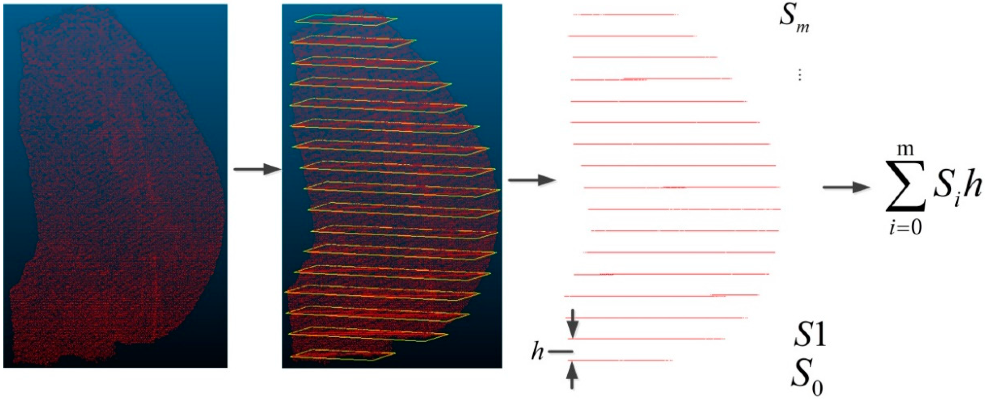
Funding

This research was funded by the National Natural Science Foundation of China (NSFC), under grant number 41971352.

Data Availability Statement

Data sharing is not applicable to this article.

Acknowledgments

The authors are very grateful to the many people who provided feedback on the article, and to the Large-Scale Environment Remote Sensing Platform (Facility No. 16000009, 16000011, 16000012) provided by Wuhan University. and the support provided by the Surveying and Mapping Institute Lands and Resource Department of Guangdong Province, Guangzhou. Special thanks go out to the editors and reviewers for providing invaluable insights into our article.

Conflicts of Interest

The authors declare no conflict of interest.

References

  1. Curless, B.; Levoy, M. A volumetric method for building complex models from range images. In Proceedings of the 23rd Annual Conference on Computer Graphics and Interactive Techniques, New Orleans, LA, USA, 4–9 August 1996; pp. 303–312. [Google Scholar]
  2. Artzet, S.; Chen, T.W.; Chopard, J.; Brichet, N.; Mielewczik, M.; Cohen-Boulakia, S.; Pradal, C. Phenomenal: An automatic open source library for 3D shoot architecture reconstruction and analysis for image-based plant phenotyping. bioRxiv 2019. bioxriv: 805739. [Google Scholar] [CrossRef]
  3. Xu, Z.; Xu, E.; Wu, L.; Liu, S.; Mao, Y. Registration of terrestrial laser scanning surveys using terrain-invariant regions for measuring exploitative volumes over open-pit mines. Remote Sens. 2019, 11, 606. [Google Scholar] [CrossRef]
  4. Szostak, M.; Pająk, M. LiDAR Point Clouds Usage for Mapping the Vegetation Cover of the “Fryderyk” Mine Repository. Remote Sens. 2022, 15, 201. [Google Scholar] [CrossRef]
  5. Zheng, X.; He, X.; Yang, X.; Ma, H.; Yu, Z.; Ren, G.; Li, J.; Zhang, H.; Zhang, J. Terrain point cloud assisted GB-InSAR slope and pavement deformation differentiate method in an open-pit mine. Sensors 2020, 20, 2337. [Google Scholar] [CrossRef]
  6. Esposito, G.; Mastrorocco, G.; Salvini, R.; Oliveti, M.; Starita, P. Application of UAV photogrammetry for the multi-temporal estimation of surface extent and volumetric excavation in the Sa Pigada Bianca open-pit mine, Sardinia, Italy. Environ. Earth Sci. 2017, 76, 103. [Google Scholar] [CrossRef]
  7. Tong, X.; Liu, X.; Chen, P.; Liu, S.; Luan, K.; Li, L.; Liu, S.; Liu, X.; Xie, H.; Jin, Y.; et al. Integration of UAV-based photogrammetry and terrestrial laser scanning for the three-dimensional mapping and monitoring of open-pit mine areas. Remote Sens. 2015, 7, 6635–6662. [Google Scholar] [CrossRef]
  8. Wajs, J. Research on surveying technology applied for DTM modelling and volume computation in open pit mines. Min. Sci. 2015, 22, 75–83. [Google Scholar]
  9. Wang, Y.; Tu, W.; Li, H. Fragmentation calculation method for blast muck piles in open-pit copper mines based on three-dimensional laser point cloud data. Int. J. Appl. Earth Obs. Geoinf. 2021, 100, 102338. [Google Scholar] [CrossRef]
  10. Liu, Q.; Duan, Q.; Zhao, P.; Ren, H.; Duan, H.; Liu, G.; Wang, Z.; Duan, Z.; Qin, L. Summary of calculation methods of engineering earthwork. In Journal of Physics: Conference Series; IOP Publishing: Bristol, UK, 2021; Volume 1802, p. 032002. [Google Scholar]
  11. Liu, X.; Zhu, W.; Lian, X. Monitoring mining surface subsidence with multi-temporal three-dimensional unmanned aerial vehicle point cloud. Remote Sens. 2023, 15, 374. [Google Scholar] [CrossRef]
  12. Kim, J.; Lee, S.; Seo, J.; Lee, D.-E.; Choi, H.S. The integration of earthwork design review and planning using UAV-based point cloud and BIM. Appl. Sci. 2021, 11, 3435. [Google Scholar] [CrossRef]
  13. Fernández-Sarría, A.; Martínez, L.; Velázquez-Martí, B.; Sajdak, M.; Estornell, J.; Recio, J.A. Different methodologies for calculating crown volumes of Platanus hispanica trees using terrestrial laser scanner and a comparison with classical dendrometric measurements. Comput. Electron. Agric. 2013, 90, 176–185. [Google Scholar] [CrossRef]
  14. Wang, Y.; Fan, Z.; You, Y. Application Research of Earth Volume Calculation Based on 3D Laser Point Cloud Data; IOP Conference Series: Materials Science and Engineering; IOP Publishing: Bristol, UK, 2020; Volume 780, p. 032050. [Google Scholar]
  15. Yang, X.; Huang, Y.; Zhang, Q. Automatic stockpile extraction and measurement using 3D point cloud and multi-scale directional curvature. Remote Sens. 2020, 12, 960. [Google Scholar] [CrossRef]
  16. Miranda-Fuentes, A.; Llorens, J.; Gamarra-Diezma, J.L.; Gil-Ribes, J.A.; Gil, E. Towards an optimized method of olive tree crown volume measurement. Sensors 2015, 15, 3671–3687. [Google Scholar] [CrossRef] [PubMed]
  17. Saha, K.K.; Tsoulias, N.; Weltzien, C.; Zude-Sasse, M. Estimation of vegetative growth in strawberry plants using mobile LiDAR laser scanner. Horticulturae 2022, 8, 90. [Google Scholar] [CrossRef]
  18. Zolanvari, S.I.; Laefer, D.F. Slicing Method for curved façade and window extraction from point clouds. ISPRS J. Photogramm. Remote Sens. 2016, 119, 334–346. [Google Scholar] [CrossRef]
  19. Li, H.; Qian, Y.; Cao, P.; Yin, W.; Dai, F.; Hu, F.; Yan, Z. Calculation method of surface shape feature of rice seed based on point cloud. Comput. Electron. Agric. 2017, 142, 416–423. [Google Scholar] [CrossRef]
  20. Zhi, Y.; Zhang, Y.; Chen, H.; Yang, K.; Xia, H. A method of 3d point cloud volume calculation based on slice method. In Proceedings of the 2016 International Conference on Intelligent Control and Computer Application (ICCA 2016), Zhengzhou, China, 16–17 January 2016; pp. 155–158. [Google Scholar]
  21. Chang, W.C.; Wu, C.H.; Tsai, Y.H.; Chiu, W. Object volume estimation based on 3d point cloud. In Proceedings of the 2017 International Automatic Control Conference (CACS), Pingtung, Taiwan, 12–15 November 2017; pp. 1–5. [Google Scholar]
  22. Yu, X.; Cheng, Z.; Zhang, Y.; Ou, L. Point cloud modeling and slicing algorithm for trajectory planning of spray painting robot. Robotica 2021, 39, 2246–2267. [Google Scholar] [CrossRef]
  23. Li, B.; Wei, J.; Wang, L. A comparative analysis of two points cloud volume calculation methods. Int. J. Remote Sens. 2019, 40, 3227–3246. [Google Scholar] [CrossRef]
  24. Liu, J.J.; Li, H.J. Volume measurement of irregular objects based on improved point cloud slicing method. Acta Opt. Sin. 2021, 41, 133–145. [Google Scholar]
  25. Oh, S.; Lee, D.; Kim, M.; Kim, T.; Cho, H. Building component detection on unstructured 3D indoor point clouds using RANSAC-based region growing. Remote Sens. 2021, 13, 161. [Google Scholar] [CrossRef]
  26. Shi, B.Q.; Liang, J.; Liu, Q. Adaptive simplification of point cloud using k-means clustering. Comput.-Aided Des. 2011, 43, 910–922. [Google Scholar] [CrossRef]
  27. Zhang, S.; Cui, S.; Ding, Z. Hypergraph spectral clustering for point cloud segmentation. IEEE Signal Process. Lett. 2020, 27, 1655–1659. [Google Scholar] [CrossRef]
  28. Golovinskiy, A.; Funkhouser, T. Min-cut based segmentation of point clouds. In Proceedings of the 2009 IEEE 12th International Conference on Computer Vision Workshops, ICCV Workshops, Kyoto, Japan, 27 September–4 October 2009; pp. 39–46. [Google Scholar]
  29. Liu, H.; Song, R.; Zhang, X. Point cloud segmentation based on Euclidean clustering and multi-plane extraction in rugged field. Meas. Sci. Technol. 2021, 32, 095106. [Google Scholar] [CrossRef]
  30. Yan, Z.; Liu, R.; Cheng, L.; Zhou, X.; Ruan, X.; Xiao, Y. A concave hull methodology for calculating the crown volume of individual trees based on vehicle-borne LiDAR data. Remote Sens. 2019, 11, 623. [Google Scholar] [CrossRef]
Figure 1. Schematic diagram of point cloud slicing method. The large irregular object is first divided into a series of parallel slices. Then, by calculating the area of the polygons within each slice, the method sums up these areas multiplied by the interval between the slices to obtain an approximate volume value.
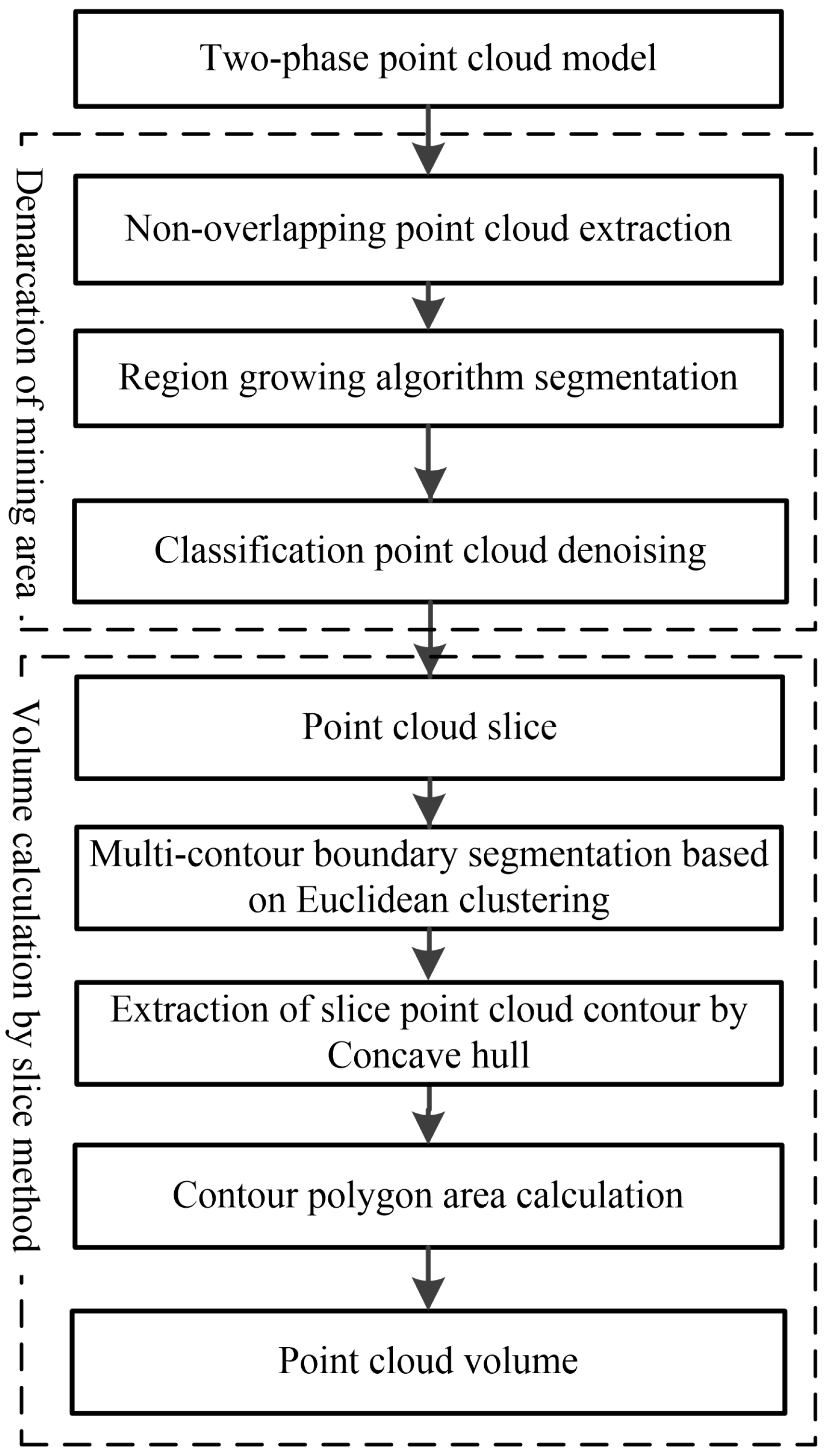
Remotesensing 15 05006 g001
Figure 2. A flow chart of the volume measurement by the cloud slicing method in an open-pit mine. To begin with, the segmentation of irregular bodies takes place. Specifically, this involves the extraction of non-overlapping regions, which effectively identify the mining zones. Subsequently, a region growing algorithm is employed to subdivide the mining zones into numerous irregular bodies. Finally, a point cloud denoising process is carried out. Following this, the proposed enhanced point cloud slicing algorithm is employed to sequentially calculate the volume of each irregular body. The results of these individual volume calculations are then aggregated to determine the overall mining volume.
Remotesensing 15 05006 g002
Figure 3. A sketch map of extraction of the mining area. Commence by extracting the non-overlapping area of the Phase 2 point cloud in comparison to the Phase 1 point cloud. Subsequently, retrieve the non-overlapping area of the Phase 1 point cloud concerning the Phase 2 point cloud. The culmination of these outcomes shapes the mining area, as highlighted by the red annotation within the illustration.
Remotesensing 15 05006 g003
Figure 4. The primary reasons for anomalies in multi-contour boundary extraction using the bidirectional nearest point search method are as follows. (a) The distances between the contours of multiple contour boundaries are excessively far, resulting in the formation of a connected anomalous edge, as illustrated in (a). (b) Irregularities in the extraction of contour polygons arise from uneven point cloud density, as depicted in (b).
Remotesensing 15 05006 g004
Figure 5. Illustration of the combined Delaunay-based concave hull algorithm for contour extraction. Each slice’s point cloud undergoes Delaunay triangulation. Following this, the boundaries of triangles forming convex polygons are identified. For each recognized convex polygon contour, the concave hull algorithm is employed to combine the contours into a unified boundary.
Remotesensing 15 05006 g005
Figure 6. The experimental data. (a) Point cloud data from the first phase of the first group. (b) Point cloud data from the second phase of the first group. (c) Point cloud data from the first phase of the second group. (d) Point cloud data from the second phase of the second group.
Remotesensing 15 05006 g006
Figure 7. Non-overlapping point cloud extraction results. (a) First phase of the original point cloud in the first group. (b) First phase of non-overlapping point clouds in the first group. (c) Top view of the merging of non-overlapping point clouds in the first group during two periods. (d) Second phase of the original point cloud in the first group. (e) Second non-overlapping point cloud in the first group. (f) Bottom view of the merging of non-overlapping point clouds in the first group during two periods. (g) First phase of the original point cloud in the second group. (h) First phase of non-overlapping point clouds in the second group. (i) Top view of the merging of non-overlapping point clouds in the second group during two periods. (j) Second phase of the original point cloud in the second group. (k) Second non-overlapping point cloud in the second group. (l) Bottom view of the merging of non-overlapping point clouds in the second group during two periods.
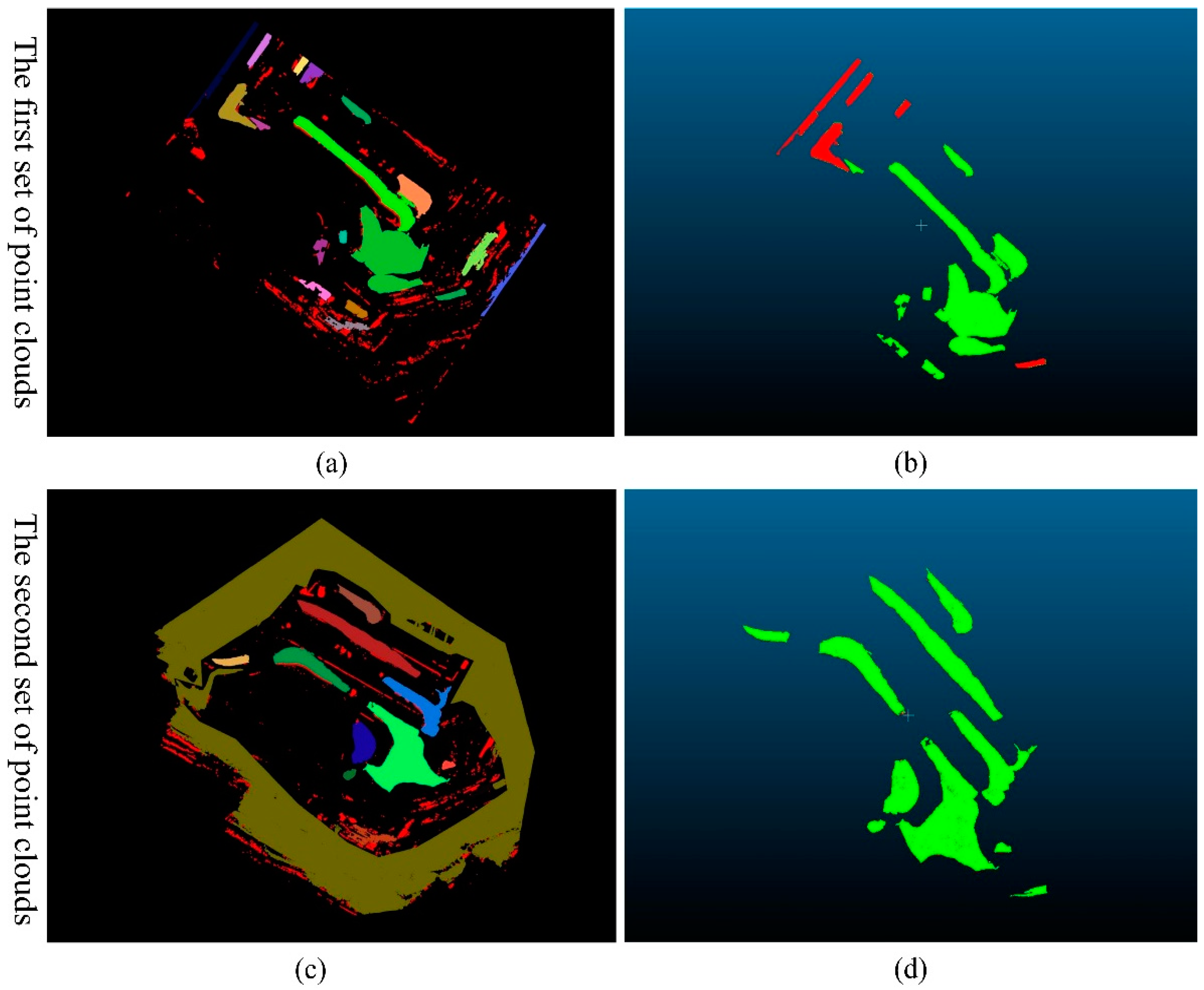
Remotesensing 15 05006 g007
Figure 8. Point cloud preprocessing results. (a) The first group of point cloud classification results. (b) The first group of point cloud denoising results. (c) The second group of point cloud classification results. (d) The second group of point cloud denoising results. It is important to highlight that, within the classification results, as depicted in (a,c), distinct colors have been employed to designate various categories, each corresponding to an autonomous irregular body. In terms of denoising results, as depicted in (b,d), it is evident that there are significantly fewer noise points in comparison to those present in (a,c).
Remotesensing 15 05006 g008
Figure 9. Partial point cloud data and their slicing results. (a) Unsegmented point cloud dataset. (b) Point cloud dataset after slicing in the cutting plane illustrated in (a), showcasing the existence of both single-contour boundaries, as observed at d = 165, and multi-contour boundaries, as evidenced by d = 137.
Remotesensing 15 05006 g009
Figure 10. The multi-contour boundary extraction results. The point clouds within the slices might encompass multiple contours. To address this, the Euclidean clustering method is applied for the segmentation of these numerous contours. Subsequently, the concave hull algorithm is employed to independently extract the boundaries of each contour from the point cloud. Taking the instance of d = 38 in the illustration, the Euclidean clustering algorithm segregates the left and right contours within the slice. Following contour extraction, two closed polygons are accurately generated.
Remotesensing 15 05006 g010
Figure 11. Comparison of multi-contour boundary extraction results using different methods within the sliced point clouds. (a) Scatter profile of the original sliced point cloud and its default sorted contours. (b) Contours sorted using the traditional point cloud slicing method. (c) Contours sorted using the proposed enhanced point cloud slicing method. It is evident that our method provides more accurate results when dealing with uneven point cloud densities and the presence of multiple contours within the slices (e.g., d = 138, d = 37).
Remotesensing 15 05006 g011
Figure 12. The chosen point cloud data and their respective 3D modeled results. (a) Depicts the first group of point cloud data. (a1a8) Correspond to the modeled outcomes of the eight subsets of point clouds within (a). (b) Represents the second group of point cloud data. Likewise, (b1b9) correspond to the modeled outcomes of all irregular bodies within (b).
Remotesensing 15 05006 g012
Table 1. The results of partial position-sliced cross-sectional areas for the same selected region.
NoSlicing PositionActual Area/m2NoSlicing PositionActual Area/m2
1d = 9.5941.395d = 114.53928.04
2d = 381246.476d = 125.753775.72
3d = 63.52710.737d = 1372383.83
4d = 90.54109.298d = 165933.82
Table 2. Partial point cloud volume calculation results using the enhanced slicing method.
Index of SliceSlicing PositionComputed Slice Volume/m3
1d = 0.57.014
2d = 1.08.488
3d = 1.513.858
………………
768d = 376.004.694
769d = 376.501.940
Table 3. Area calculation accuracy between the proposed method and the traditional approach.
Slicing PositionActual Area/m2Traditional Point Cloud Slicing Method Area/m2Enhanced Point Cloud Slicing Method Area/m2Relative Error of the Traditional Point Cloud Slicing Method/%Relative Error of the Enhanced Point Cloud Slicing Method/%
d = 9.5941.39950.65950.650.980.98
d = 381246.47946.351260.7324.081.14
d = 63.52710.732563.182735.545.440.92
d = 90.54109.292869.724144.2730.170.85
d = 114.53928.043937.93943.130.250.38
d = 125.753775.723804.143804.140.750.75
d = 1372383.831485.852387.2637.670.14
d = 165933.82941.54941.540.830.83
Table 4. Comparison of results and accuracy for calculating the volume of the first group of point cloud data.
Point Cloud Serial NumberModeling Method Volume/m3Traditional Point Cloud Slicing Method Volume/m3Slice Method Volume/m3Relative Error of the Traditional Point Cloud Slicing Method/%Relative Error of the Enhanced Point Cloud Slicing Method/%
a136,208.1933,799.4436,025.306.650.51
a2414,880.44402,798.03420,520.212.911.36
a317,048.5013,097.4916,623.4723.182.49
a4108,175.2897,901.53107,930.939.500.23
a525,438.9722,395.6224,712.3311.962.86
a68410.147047.138394.6316.210.18
a710,922.427511.0811,103.4831.231.66
a8820,913.03726,134.21835,475.1711.551.77
Table 5. Comparison of results and accuracy for calculating the volume of the second group of point cloud data.
Point Cloud Serial NumberModeling Method Volume/m3Traditional Point Cloud Slicing Method Volume/m3Slice Method Volume/m3Relative Error of the Traditional Point Cloud Slicing Method/%Relative Error of the Enhanced Point Cloud Slicing Method/%
b1446,229.99352,648.54434,473.9720.972.63
b277,430.8272,141.6776,804.896.830.81
b3180,884.95169,572.10180,961.126.250.04
b4170,941.48159,884.40169,831.036.470.65
b5272,074.44255,381.54271,756.676.140.12
b6170,232.95163,264.25166,888.614.091.96
b722,383.5518,142.1722,509.8318.950.56
b86969.856222.127055.8110.731.23
b910,090.019429.14 9939.456.551.49
Table 6. Comparison of different point cloud boundary extraction algorithms.
Point Cloud Slice NumberNumber of Contours in the SliceThe Time of the Bidirectional Nearest Neighbor Search Algorithm/msThe Time of the Polygon Classification and Reconstruction Method/msThe Time of the Concave Hull Algorithm (Proposed Method)/ms
s111.96902.43191.8616
s210.78211.47550.9968
s331.63241.99761.9851
s421.89924.07012.0311
s521.99361.82531.9951
s611.82812.38411.9944
s710.99911.23470.9973
Table 7. Comparison of computational time for algorithms.
Point Cloud Serial NumberThe Time of the Traditional Point Cloud Slicing Method/sThe Time of the Enhanced Point Cloud Slicing Method/sPoint Cloud Serial NumberThe Time of the Traditional Point Cloud Slicing Method/sThe Time of the Enhanced Point Cloud Slicing Method/s
a114.0312.35b1396.68374.05
a2375.53365.78b235.6333.12
a34.873.58b3118.2116.37
a461.2656.46b486.3282.14
a515.5414.63b5219.65214.48
a62.981.71b647.7544.56
a78.236.82b74.013.51
a8582.95568.31b81.010.93
Disclaimer/Publisher’s Note: The statements, opinions and data contained in all publications are solely those of the individual author(s) and contributor(s) and not of MDPI and/or the editor(s). MDPI and/or the editor(s) disclaim responsibility for any injury to people or property resulting from any ideas, methods, instructions or products referred to in the content.

