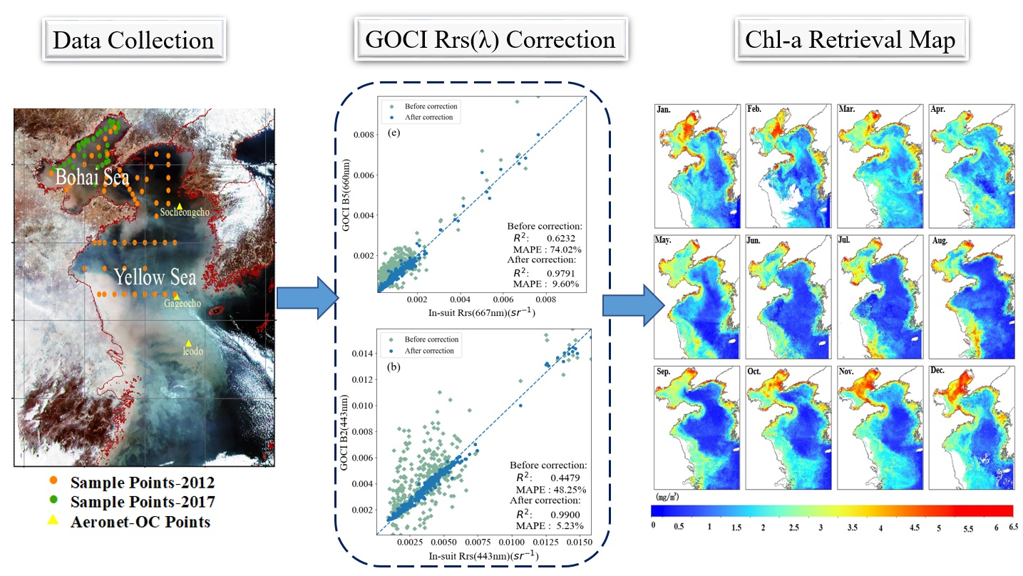
Quantitative Retrieval of Chlorophyll-a Concentrations in the Bohai–Yellow Sea Using GOCI Surface Reflectance Products

Abstract

As an environmental parameter, the chlorophyll-a concentration (Chl-a) is essential for monitoring water quality and managing the marine ecosystem. However, current mainstream Chl-a inversion algorithms have limited accuracy and poor spatial and temporal generalization in Case II waters. In this study, we constructed a quantitative model for retrieving the spatial and temporal distribution of Chl-a in the Bohai–Yellow Sea area using Geostationary Ocean Color Imager (GOCI) spectral remote sensing reflectance ($R_{rs}\left(\lambda \right)$) products. Firstly, the GOCI $R_{rs}\left(\lambda \right)$ correction model based on measured spectral data was proposed and evaluated. Then, the feature variables of the band combinations with the highest correlation with Chl-a were selected. Subsequently, Chl-a inversion models were developed using three empirical ocean color algorithms (OC4, OC5, and YOC) and four machine learning methods: BP neural network (BPNN), random forest (RF), AdaBoost, and support vector regression (SVR). The retrieval results showed that the machine learning methods were much more accurate than the empirical algorithms and that the RF model retrieved Chl-a with the best performance and the highest prediction accuracy, with a determination coefficient R² of 0.916, a root mean square error (RMSE) of 0.212 mg$·$m⁻³, and a mean absolute percentage error (MAPE) of 14.27%. Finally, the Chl-a distribution in the Bohai–Yellow Sea using the selected RF model was derived and analyzed. Spatially, Chl-a was high in the Bohai Sea, including in Laizhou Bay, Bohai Bay, and Liaodong Bay, with a value higher than 4 mg$·$m⁻³. Chl-a in the Bohai Strait and northern Yellow Sea was relatively low, with a value of less than 3 mg$·$m⁻³. Temporally, the inversion results showed that Chl-a was considerably higher in winter and spring compared to autumn and summer. Diurnal variation retrieval effectively demonstrated GOCI’s potential as a capable tool for monitoring intraday changes in chlorophyll-a concentrations.

1. Introduction

The chlorophyll-a concentration (Chl-a, mg$·$m⁻³) is one of the most essential parameters for the study of phytoplankton dynamics, the carbon cycle, and eutrophication in global oceans including coastal/inland waters [1,2]. The conventional method of obtaining Chl-a involves manual stationary sampling and laboratory analysis, leading to significant spatial and temporal limitations and requiring substantial time and labor [3]. Ocean water color satellites have effectively resolved these issues, providing a significant and transformative approach for marine ecological environment monitoring [4,5,6].

The models for retrieving Chl-a in current studies can be divided into empirical or semi-empirical algorithms and artificial intelligence [7,8]. Various empirical algorithms have been developed for chlorophyll-a concentration estimation, including the empirical ocean color (OC) algorithm proposed by O’Reilly [9,10], the three-band reflectance difference method for low-nutrient seas proposed by Hu [11,12], and the normalized difference chlorophyll index (NDCI) used by Rodríguez-López et al. [13]. Cheng et al. [14] demonstrated that two-band and three-band methods are effective for estimating Chl-a in inland water with WV-2 imagery. Li et al. [15] applied a four-band model (FBA) to OLCI images, and the monthly and spatial distributions of Chl-a in Lake Xingkai were studied from 2016 to 2022. Most of these semi-analytical algorithms are applied to invert Chl-a in inland lakes and require more parameters. More advanced technologies such as artificial intelligence have been applied in Chl-a estimation [16,17]. Some approaches have been applied to Chl-a retrieval successfully, including a deep neural network (DNN) [18], a convolutional neural network [19], mixture density networks [6], a backpropagation (BP) neural network [20], and random forest (RF) [21]. Although these algorithms have achieved high inversion accuracy, challenges remain for turbid coastal or inland waters [22]. The optical properties are complex and highly variable due to the intermingled optical signals of chlorophyll, suspended sediments (SPM), and colored dissolved organic matter (CDOM). For Case II waters, it is usually too difficult to use a single algorithm to accommodate the optical complexity. Thus, to achieve accurate Chl-a retrieval, the inversion model must be developed according to the specific conditions of the sea area [23,24].

The Bohai–Yellow Sea located in north China is very rich in marine biological resources, which makes it an important part of China’s marine economy [25]. However, with the rapid development of coastal cities, human exploitation of marine resources has become increasingly frequent and has resulted in increasingly serious eutrophication of coastal water bodies [26,27]. For the Case II water body of the Bohai–Yellow Sea, it is an urgent task to monitor the ocean color and quality change in detail. So far, many scholars have established corresponding inversion models using machine learning methods for different regions [22,28,29,30], but the accuracy of these models is often limited to a specific space and time, and their spatial and temporal generalizations are not sufficient. Additionally, high accuracy reflectance data serve as a prerequisite and foundation for accurately inverting Chl-a. However, atmospheric correction for Case II water bodies poses inherent challenges [31], making it difficult to obtain precise Chl-a measurements for such water bodies.

To address the issues of Chl-a inversion in Case II waters of the Bohai–Yellow Sea, this study firstly validated and corrected the GOCI spectral remote sensing reflectance ($R_{rs}\left(\lambda \right)$) using the spectral data from the ocean color component of the Aerosol Robotic Network (AERONET-OC). Next, we constructed a quantitative retrieval model for Chl-a using in situ collected Chl-a data and corrected the GOCI reflectance products. Then, the best model was selected to retrieve Chl-a, and finally spatial and temporal variations in chlorophyll-a in the study area were evaluated and analyzed.

2. Material and Methods

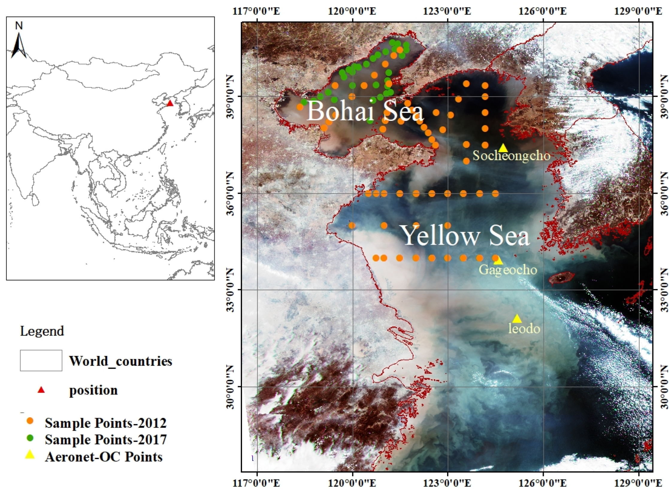
2.1. Study Area

The study area is the Bohai–Yellow Sea located in the northern part of China, which includes two parts. The north Bohai Sea lying between the Liaodong Peninsula and the Jiaozhou Peninsula is the largest inland sea in China [32] and covers 77,000 square kilometers with an average depth of 18 m. Bohai Sea is recognized for its semi-enclosed Case II water body with distinctive characteristics of high chlorophyll levels due to terrestrial inputs [33]. The south Yellow Sea spans around 380,000 square kilometers, displaying both deep and shallow sea features [34,35]. The Bohai–Yellow Sea receives nutrients and sediments from the Yellow River and Yangtze River. River runoff, upwelling, and sediment resuspension affect the hydrodynamic processes and environment of the Bohai–Yellow Sea [36]. The location and extent of the study area is shown in Figure 1.

2.2. Data Sources and Preprocessing

The time series monitoring data were obtained from the ocean color component of the AERONET-OC. The AERONET-OC has been designed to support long-term satellite ocean color investigations through cross-site measurements collected by autonomous multispectral radiometer systems deployed above water [37]. A large number of studies have used the ocean-colored data provided by AERONET-OC for data validation and algorithm evaluation [31,38,39,40]. In the study area, we selected three sites (Gageocho_Station: 33.942N, 124.593E; leodo_Station: 32.123N, 125.182E; Socheongcho: 37.423N, 124.738E) from AERONET-OC and calculated the spectral remote sensing reflectance ($R_{rs}\left(\lambda \right)$) by dividing water leaving radiances $\left(L_{wn}\right)$ by the solar constant (Equation (1)). Version 3 level 2.0 quality-assured AERONET-OC field measurements were selected as our in situ data, including $L_{wn}$ and Chl-a; all these data were downloaded from the AERONET-OC website (https://aeronet.gsfc.nasa.gov/, accessed on 10 March 2022).

$$R_{rs}\left(\lambda \right)=n{L}_{wn}\left(\lambda \right)/F_0\left(\lambda \right)$$

(1)

The measured spectra were all collected from AERONET-OC and used for the GOCI $R_{rs}\left(\lambda \right)$ correction. We also collected Bohai–Yellow Sea in situ Chl-a data in February, May, and August 2012 and in February 2017. These data were combined with the AERONET-OC site data to create Chl-a in situ datasets. The distribution of all sampling points is shown in Figure 1.

COMS is the world’s first geostationary satellite launched in June 2010. It is equipped with the GOCI (Geostationary Ocean Color Imager) sensor, the observation surface range is 2500 km × 2500 km, and the latitude and longitude of the observation center is (130°E, 36°N) [41]. GOCI has a spatial resolution of 500 m and a temporal resolution of 1 h and can acquire eight views per day [25]. Based on the purpose of observation of ocean color, GOCI sets six visible bands centered at λ = 412, 443, 490, 555, 660, and 680 nm and two near-infrared (NIR) bands centered at λ = 745 and 865 nm. In this study, we used Level 2 images from the GOCI sensor, which reflect atmospheric correction and can be downloaded from (http://kosc.kiost.ac.kr/, accessed on 13 January 2022).

Given the different sampling characteristics, an appropriate spatial and temporal window must be determined based on the resolution of the satellite product and the characteristics of the water body [42]. The following criteria were used to search for the in situ satellite matching pairs [31,43]:

(1)

images with cloud coverage more than 70%, and the points under a cloud or in cloud shadows were discarded from the analysis.

(2)

a box of 3 × 3 pixels centered at the sample points was extracted.

(3)

the time difference between the field data and the GOCI overpass was within ±3 h.

After quality control with the above-mentioned criteria, we obtained 360 matching pairs of GOCI images and AERONET-OC spectral data, along with 409 matching pairs of collected Chl-a and GOCI images for subsequent modeling.

2.3. Methodology

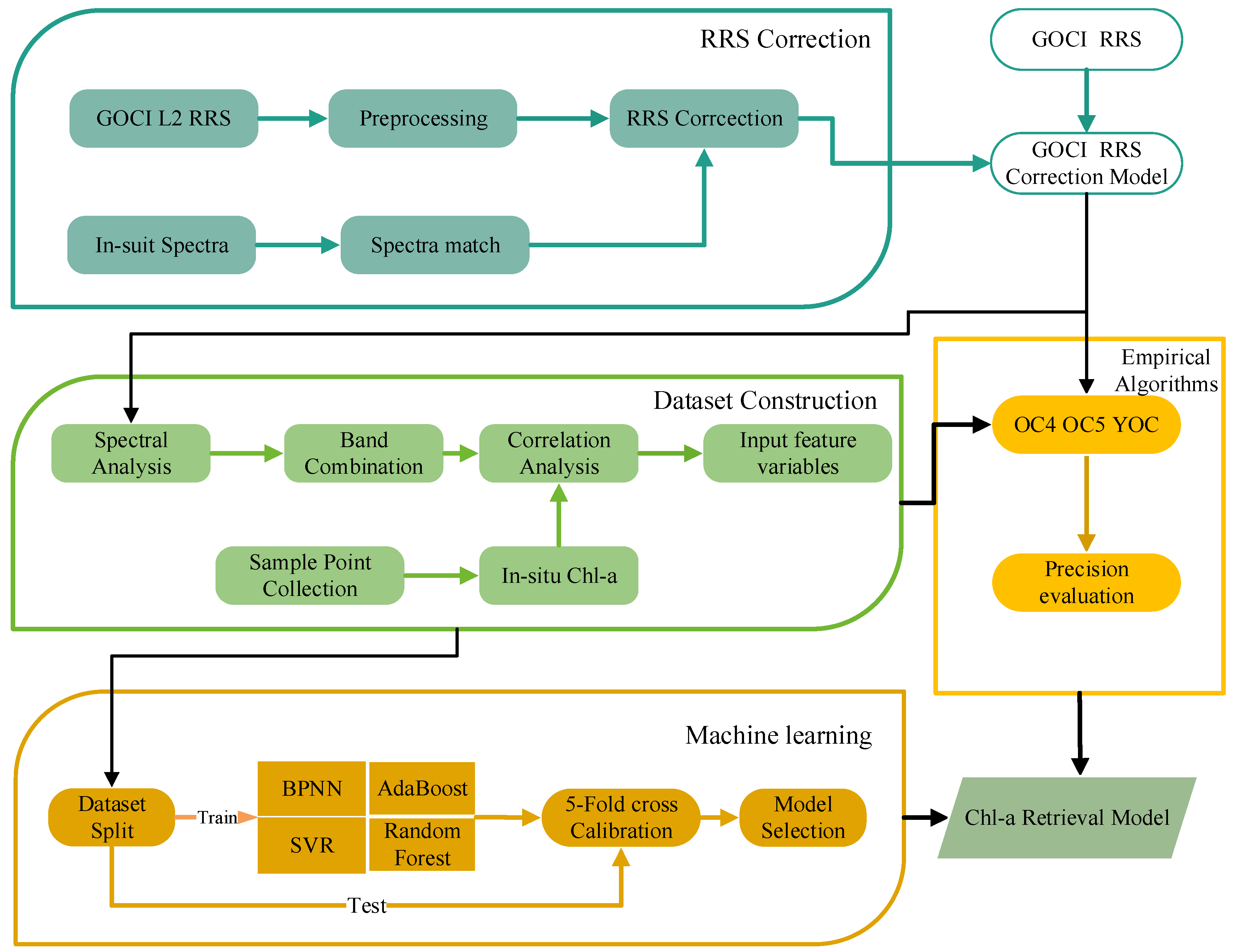
2.3.1. The Flowchart of Chl-a Retrieval Modeling

Four key steps are proposed for the construction of a Chl-a retrieval model in our research as follows:

(1)

GOCI surface remote sensing reflectance correction

(2)

Band combination and factor selection

(3)

Comparative study for Chl-a estimation modeling

(4)

Accuracy assessment and analysis of retrieval results

The flowchart of Chl-a retrieval modeling is shown in Figure 2.

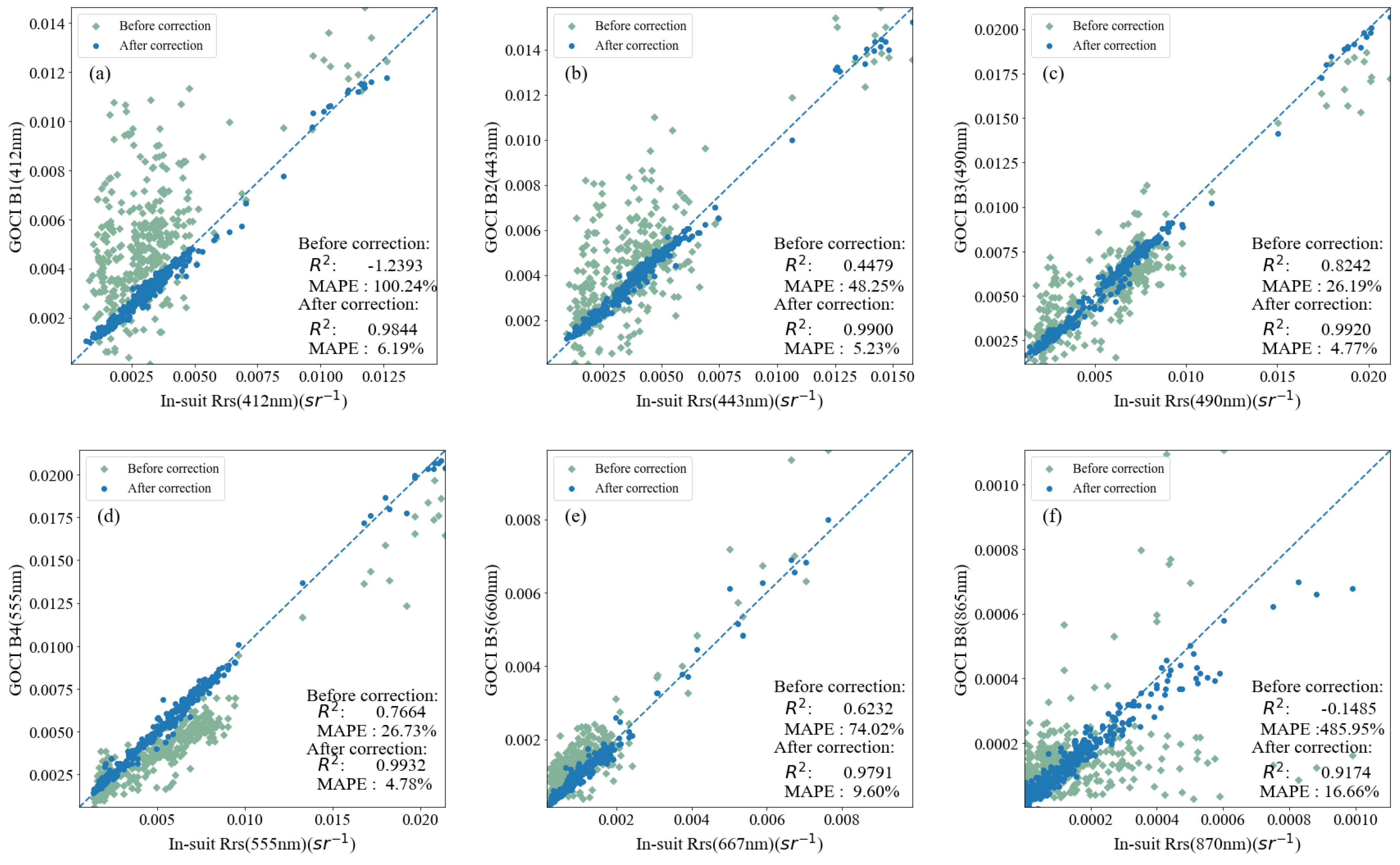
2.3.2. GOCI Spectral Remote Sensing Reflectance Correction

The accuracy of the GOCI $R_{rs}\left(\lambda \right)$ products in six spectral bands was evaluated by comparing them with the corresponding AERONET-OC measured spectral data. These bands include B1 (412 nm), B2 (443 nm), B3 (490 nm), B4 (555 nm), B5 (660 nm), and B8 (865 nm). AERONET-OC has corresponding spectral data for these bands, except for the B6 (680 nm) and B7 (745 nm) bands. From the comparison results, the spectrum of GOCI at 490 nm is the most consistent with the measured spectral data (R² = 0.82), but there is substantial deviation from the measured results at 412 nm, 443 nm, and 865 nm, with the R² being less than 0.5. Overall, the evaluation results of the GOCI $R_{rs}\left(\lambda \right)$ products using the measured spectral data were generally consistent with a previous study [44]; good accuracy was observed for the B3, B4, and B5 bands, but poor accuracy was observed for the B1 band.

To correct the GOCI $R_{rs}\left(\lambda \right)$ products, we established a random forest regression model with measured spectral data. The input dataset comprised the GOCI $R_{rs}\left(\lambda \right)$ products of eight bands, and the corresponding outputs consisted of the measured spectral data for the matched six bands. The accuracy of the correction results was evaluated using the correlation coefficient (R²) and mean absolute percentage error (MAPE). As shown in Figure 3, it is clear that the corrected $R_{rs}\left(\lambda \right)$ products perform very well on measured spectral data with MAPE values smaller than 20% and R² values larger than 0.9 for all bands.

2.3.3. Band Combination and Feature Variable Selection

Different input feature variables have a critical impact on the final training accuracy of machine learning [7]. We calculated Pearson’s correlation coefficients between band combinations and Chl-a; the calculation results are shown in

Table 1. The test feature variables.

Feature Name	Band Combination Formula	Pearson’s Correlation Coefficient
V1	B1/B4	−0.375
V2	B2/B4	−0.522
V3	B3/B4	−0.636
V4	B8/B5	0.001
V5	(B5 − B1)/(B5 + B1)	0.296
V6	(B5 − B2)/(B5 + B2)	0.531
V7	(B5 − B3)/(B5 + B3)	0.511
V8	(B5 − B4)/(B5 + B4)	0.217
V9	(B5 − B8)/(B5 + B8)	−0.029
V10	(B2 − B1)/(B2 + B1)	−0.114
V11	(B2 − B3)/(B2 + B3)	−0.204
V12	(B2 − B4)/(B2 + B4)	−0.540
V13	(B2 − B8)/(B2 + B8)	−0.217
V14	(B1 + B2)/B4	−0.448
V15	(B1 + B3)/B4	−0.513
V16	(B2 + B3)/B4	−0.593
V17	(B1 + B2 + B3)/B4	−0.519
V18	(B2 + B3)/(B4 × 2)	−0.593
V19	(B1 + B3)/(B4 × 2)	−0.513
V20	(B2 + B3)/(B4 + B5)	−0.600

. By analyzing the relationship between remote sensing reflectance and measured Chl-a values for single-band or multi-band combinations, we selected the optimal band combinations using the six corrected bands. Finally, three feature variables, namely, B3/B4, (B2 + B3)/B4, and (B2 + B3)/(B4 + B5) were selected to build the inverse model of Chl-a based on machine learning methods.

2.3.4. Chlorophyll-a Retrieval Algorithms

To determine the optimal chlorophyll-a retrieval model for the Bohai–Yellow Sea, this study compared three empirical algorithms (OC4, OC5, YOC) and four machine learning algorithms.

(1)

Empirical ocean color algorithms

In this study, OC4, OC5, and YOC were investigated as empirical algorithms to estimate the Chl-a in the Bohai–Yellow Sea. O’Reilly [9] proposed a well-known empirical approach, where a sequencing blue-to-green ratio of $R_{rs}\left(\lambda \right)$ statistically related to Chl-a via a polynomial expression; this algorithm is called OC-X, where X is the number of bands, and was used in the function. The functional form of the OC-X algorithms is given as follows:

$${log}_{10}\left[CHL\right]=c_{0+}{c}_1{log}_{10}X+c_2{log}^2{}_{10}X+c_3{log}^3{}_{10}X+c_4{log}^4{}_{10}X$$

(2)

where for OC4:

$$X_{OC4}=\max \left(R_{rs}\left(412\right),R_{rs}\left(443\right),R_{rs}\left(490\right)\right)/R_{rs}\left(555\right)$$

(3)

where for OC5:

$$X_{OC5}=\max \left(R_{rs}\left(412\right),R_{rs}\left(443\right),R_{rs}\left(490\right),R_{rs}\left(555\right)\right)/R_{rs}\left(660\right)$$

(4)

The YOC algorithm was first proposed by Tassan [45]; Siswanto [46] modified the parameters in the original YOC algorithm in 2011 based on a decade of measured remote sensing reflectance and Chl-a data for the East China Sea, Yellow Sea. It is a quadratic polynomial algorithm using the multi-band ratios of 412 nm, 443 nm, 490 nm, and 555 nm. The expression of the algorithm is as follow:

$$Ch{l}_a={10}^{\left[c1-c2\times {log}_{10}\left(R\right)-c3\times lo{g}^2{}_{10}\left(R\right)\right]},$$

(5)

$$R=\frac{R_{rs} \left(443\right)}{R_{rs} \left(555\right)}{[\frac{R_{rs} \left(412\right)}{R_{rs} \left(490\right)}]}^{c4},$$

(6)

(2)

Machine learning algorithms

Four types of machine learning algorithms were assessed in this comparative study: AdaBoost, support vector regression (SVR), random forest (RF), and backpropagation neural network (BPNN). AdaBoost improves prediction accuracy by fitting weak learners to modified data, combining their predictions through weighted voting or summing, and adjusting weights based on prediction errors in regression problems [47,48]. RF, as an ensemble learning method, consists of multiple decision trees, each trained on randomly selected feature and sample subsets. The final prediction is obtained by combining the predictions of individual trees through averaging or voting [49,50]. The BPNN algorithm is a multilayered feed-forward network trained according to the backpropagation algorithm, which is divided into input layers, hidden layers, and output layers [51]. SVR finds an optimal linear classification hyperplane by mapping data to a high-dimensional space using an inner product function [52]. For regression, support vector regression aims to find a regression plane that closely fits the data points with a tolerance margin [53,54]. They are effective for solving prediction problems and capturing complex patterns in data.

We utilized collected datasets to train these models, and the final parameter tuning results of each machine learning algorithm are shown in

Table 2. Parameter settings of the machine learning models.

Machine Learning Model	* Parameter Settings
Random Forest	Number of decision trees (k): 150 Max depth: 20 Number of features (m): 3 Min samples split: 10
BPNN	Hidden layer neuron function: log S-type function Output function: linear function Strength of the L2 regularization term: 0.001 Training function: momentum BP algorithm with variable learning rate Number of iterations: 1000
AdaBoost	Base estimator: decision tree Number of estimators: 150 Learning_rate: 0.05 Loss: linear
SVM	Penalty parameter: 10 Epsilon: 0.1 Gamma: 1 Kernel function: rbf

* The other parameters: default settings.

.

2.3.5. Accuracy Evaluation

The coefficient of determination (R²), root mean square error (RMSE), mean absolute percentage error (MAPE), and mean absolute error (MAE) were used to quantitatively evaluate the performance of the retrieval model. R², RMSE, and MAPE are common metrics for assessing the performance of models based on the original data distribution; R² indicates the fit of the model, and a value closer to 1.0 indicates a better fit; and MAE computed in log-transformed space is believed to provide a good assessment of the algorithms for the log-normal distributions of Chl-a [16,55]. These metrics are defined in the following equations:

$$R^2=1-\frac{{{\displaystyle \sum }}_{i=1}^n{\left(X_i-Y_i\right)}^2}{{{\displaystyle \sum }}_{i=1}^n{\left(X_i-{\overline{Y}}_i\right)}^2},$$

(7)

$$RMSE=\sqrt{\frac{{{\displaystyle \sum }}_{i=1}^n{\left(X_i-Y_i\right)}^2}{n}},$$

(8)

$$MAE={10}^{\wedge }\left(\frac{{{\displaystyle \sum }}_{i=1}^n\left|{\log }_{10}\left(X_i\right)-{\log }_{10}\left(Y_i\right)\right|}{n}\right),$$

(9)

$$MAPE=\frac{1}{n}{\displaystyle \sum }_{i=1}^n\left|\frac{X_i-Y_i}{Y_i}\right|\times 100\%,$$

(10)

where $Y_i$ is the measured value; ${\overline{Y}}_i$ is the mean of the measured value; $X_i$ is the predicted value; the subscript $i$ denotes individual data points; and $n$ is the sample size.

3. Results

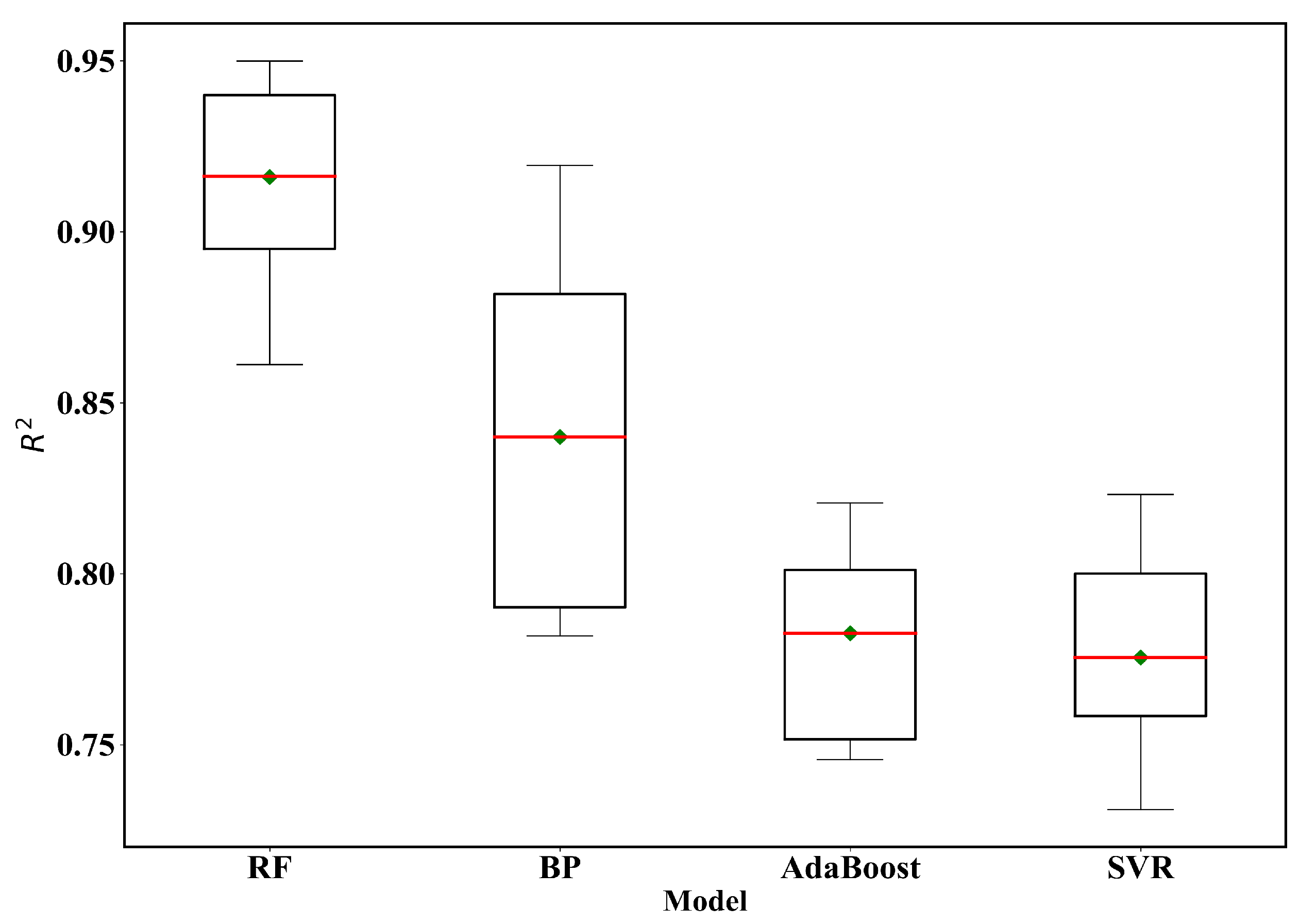
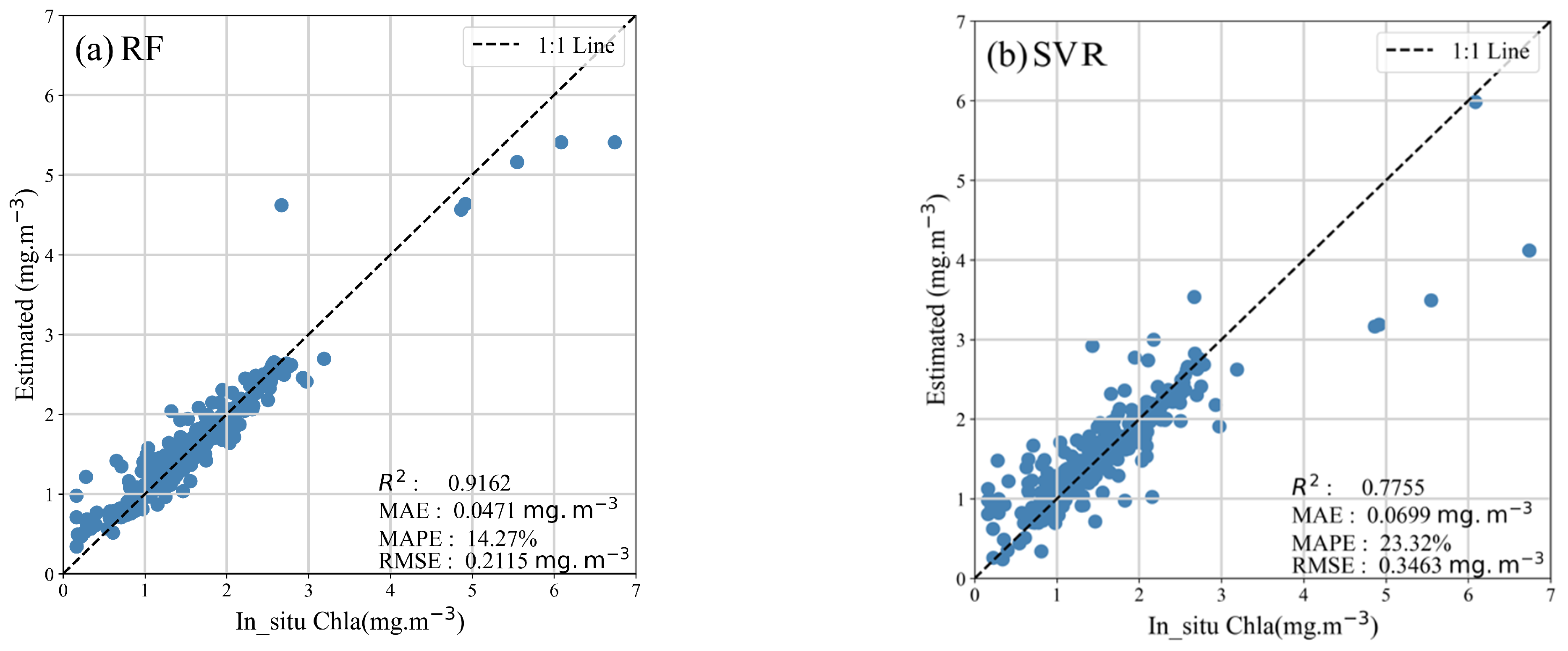
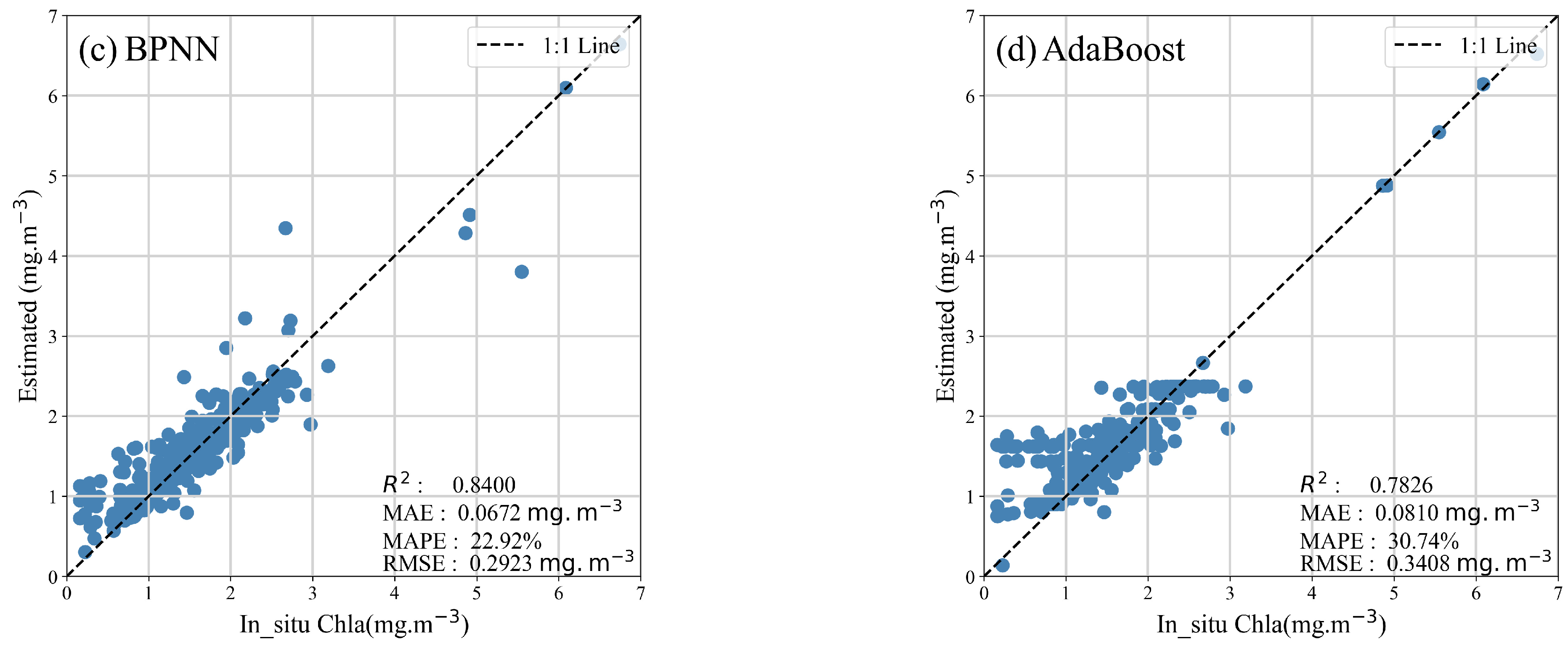
3.1. Chl-a Retrieval Model Validation

The modeling dataset was randomly divided into two parts; 70% of the data from measured sampling points were utilized to build three empirical models, and the remaining 30% of the data were set aside for accuracy verification after modeling. The coefficients of OC4 and OC5 were updated by regression in these methods, while YOC’s original coefficients remained unchanged. This process resulted in the establishment of the empirical Chl-a inversion model. The model details and accuracy are shown in

Table 3. Linear model and accuracy of chlorophyll-a concentration inversion.

Algorithms	Formula	R2	$\mathbf{RMSE}(\mathbf{mg}·$m−3)	MAPE (%)
OC4	$c0,c1, c2,c3, c4=$ $0.2555,-2.3745, 1.9381, 0.4004,-30.335$	0.581	0.688	40.269
OC5	$c0,c1, c2,c3, c4=$ $0.2975,-0.7803, 5.5591,-9.5642,4.5081$	0.418	1.055	70.534
YOC	$c1, c2,c3, c4=$ $0.342, 2.511, 0.277,-1.012$	0.509	0.524	50.134

.

K-fold cross-validation was adopted for machine learning model evaluation: a model was trained for each of the k possible training test splits, and the reported values for R² and RMSE were the average of these k runs. In this study, the chosen value for k was 5. The validation results of the four machine learning models are shown in

Table 4. Mean values for the evaluated metrics in the cross-validation step.

Model	R2	MAE (mg/m3)	$\mathbf{RMSE}(\mathbf{mg}·$m−3)	MAPE (%)
Random Forest	0.916	0.047	0.212	14.27
BPNN	0.840	0.067	0.292	22.92
AdaBoost	0.783	0.081	0.341	30.74
SVM	0.776	0.070	0.346	23.32

. We also visualized the results of the four machine learning model cross-validations by plotting box plots, as shown in Figure 4.

Through a comprehensive comparison and analysis of all models, we found that the inversion accuracy of the empirical algorithms is lower than that of the machine learning algorithms in the study area, R² of the OC5 is less than 0.5, and the accuracy of the OC4 and YOC have been improved to some extent, but it cannot reach the normal accuracy requirement which is higher than 0.65. The machine learning models used in this study show significant improvement in accuracy compared to the empirical models. Specifically, the BPNN has an R² of 0.84, while the RF model achieves an even higher accuracy with an improvement of 0.076 compared to the R² of the BPNN model. These results suggest that the machine learning model provides better nonlinear fitting and is more suitable for retrieving water quality parameters of Case II waters in complex environments. The comparison of the effectiveness of the above four machine learning algorithms is shown in Figure 5.

It is worth noting that the BPNN is a black-box model, which has certain limitations in its results interpretation. By contrast, the RF model also belongs to the black-box model, but it provides other effective ways to assist interpretation, making it easier to be explained. The RF results show that the R² is 0.916, the RMSE is 0.212 mg·m⁻³, and the MAPE is 14.27%.

Generally, the machine learning models, particularly the RF model, show significant improvement in accuracy compared to the empirical models, making it a promising approach for retrieving water quality parameters of Case II waters in complex environments.

3.2. Analysis of Chlorophyll-a Concentration Retrieval Results

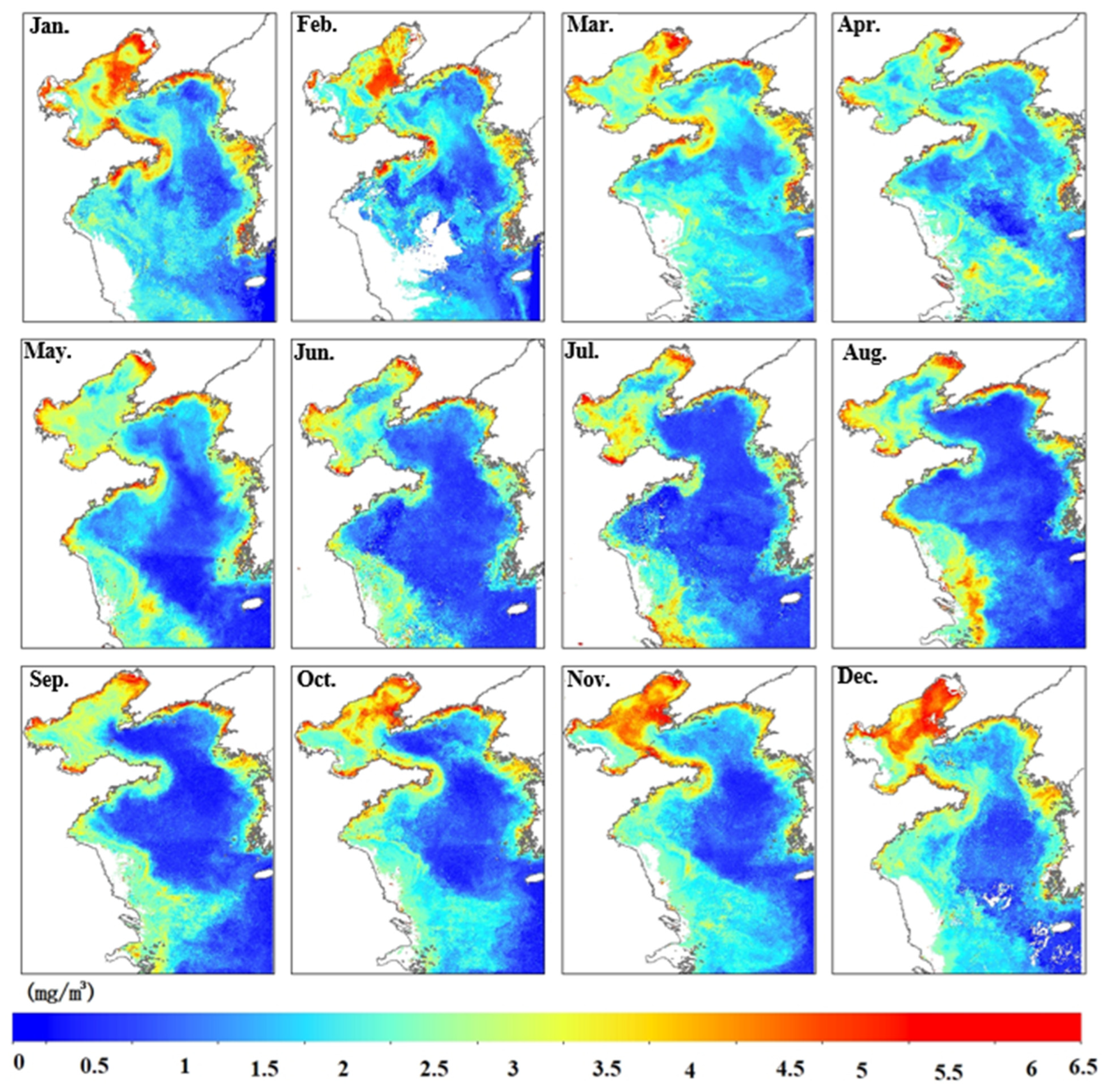
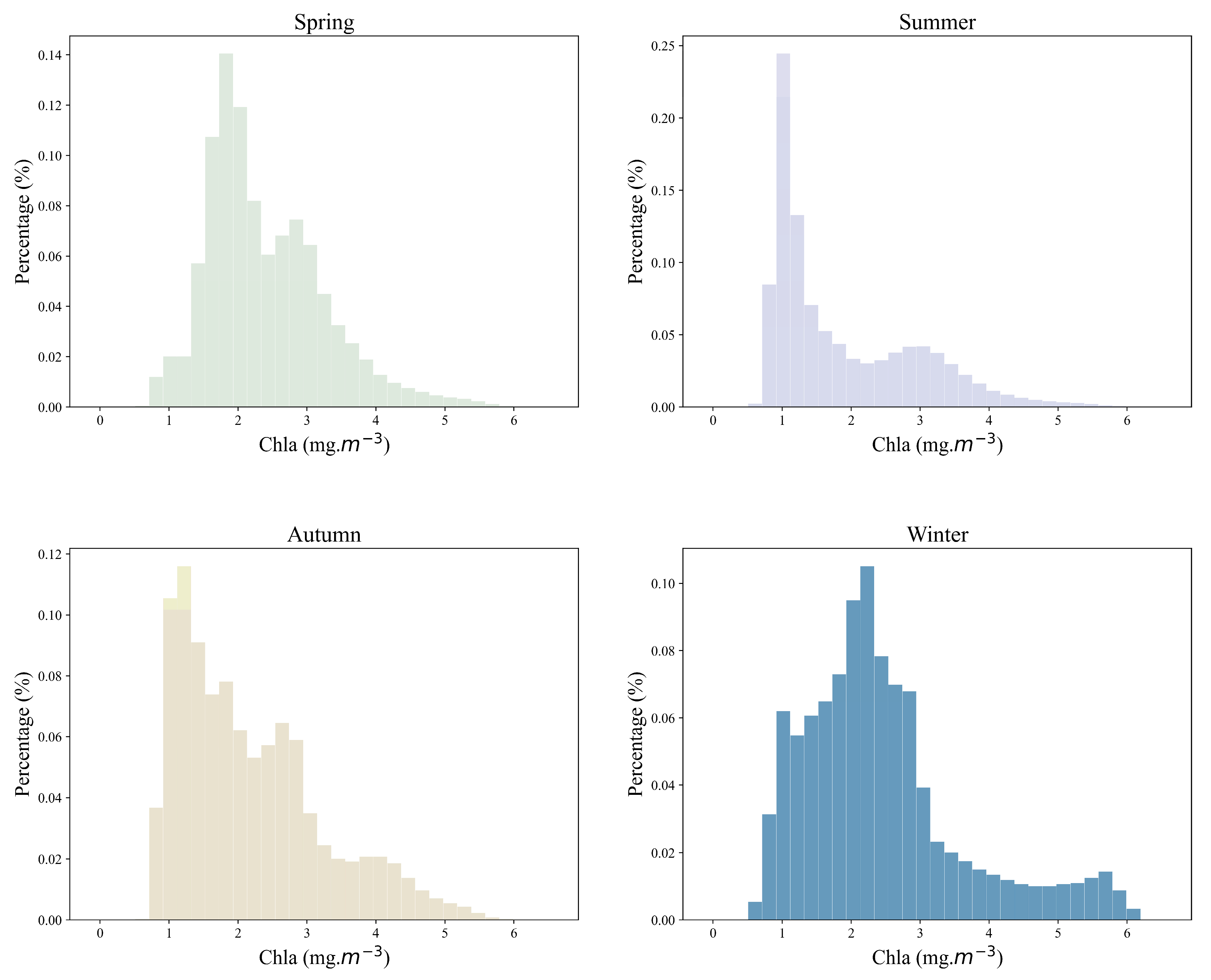
3.2.1. Spatial Distribution and Seasonal Changes in Chl-a

We used the 3:00 a.m. (UTC) image as a reference for daily Chl-a distribution. This decision is based on the fact that the solar zenith angle is at its lowest point at noon, which allows for a certain degree of neglect towards its effects. We utilized the corrected GOCI $R_{rs}\left(\lambda \right)$ and Chl-a RF inversion model to obtain the spatial distribution of Chl-a in the study area from January to December 2019. In Figure 6, the GOCI estimated values are totally consistent with in situ measurements from three AERONET-OC stations, which proves the reliability of the RF model estimated Chl-a. The daily Chl-a results were retrieved and then averaged by month to obtain 12-month average Chl-a maps. These maps are displayed in Figure 7.

Chl-a in the Bohai–Yellow Sea is mainly below 6.5 mg·m⁻³, exhibiting a pattern of increasing value with distance from the shore and decreasing value in open waters. The Chl-a in Bohai is greater than that in the Yellow Sea. High levels are typically found along the coast of Qinhuangdao, the southern portion of Laizhou Bay, the northern area of Liaodong Bay, and the coast of the northern Yellow Sea. On the other hand, the Bohai Strait and the southern Yellow Sea exhibit comparatively low levels of Chl-a. Nearshore phytoplankton growth is more abundant than that in offshore waters, primarily due to the shallower water depths in nearshore areas, greater mixing between land-source runoff and seawater, and the abundant nutrient salts from land-source runoff [56,57,58].

Based on estimated monthly Chl-a in 2019, Chl-a in the Bohai follows a monthly pattern with a peak in January, gradual decrease to a trough in August, followed by a gradual increase and another peak in December. In the coastal region of the Yellow Sea, there was a period of high Chl-a observed during the spring and summer, followed by a minimum in the winter and autumn. In the offshore region, the Chl-a time series were characterized by a distinct peak in May associated with a weak peak in December, while the minima are noted from June to September.

To investigate the seasonal pattern of Chl-a, we performed histogram analysis over four seasons: spring, summer, autumn, and winter. The statistical findings are presented in Figure 8. In this study, December, January, and February were winter; March, April, and May were spring; June, July, and August were summer; and September, October, and November were autumn. The statistical findings demonstrate that Chl-a during spring is concentrated at 1.5–3.5 mg$·$m⁻³, with two peaks at positions 2 mg$·$m⁻³ and 3 mg$·$m⁻³, respectively. The statistics of Chl-a during summer indicated a multi-peaked distribution, with the highest peak observed at 1.2 mg$·$m⁻³ and the second peak near 3 mg$·$m⁻³. Autumn and winter exhibited a clear skewed distribution, with low values taking preference: values in both seasons were concentrated in the range of 1–3 mg$·$m⁻³, with the peak values at 1.3 mg$·$m⁻³ during autumn and 2.3 mg$·$m⁻³ during winter. Additionally, the percentage of high Chl-a was significantly higher in autumn and winter than in spring and summer.

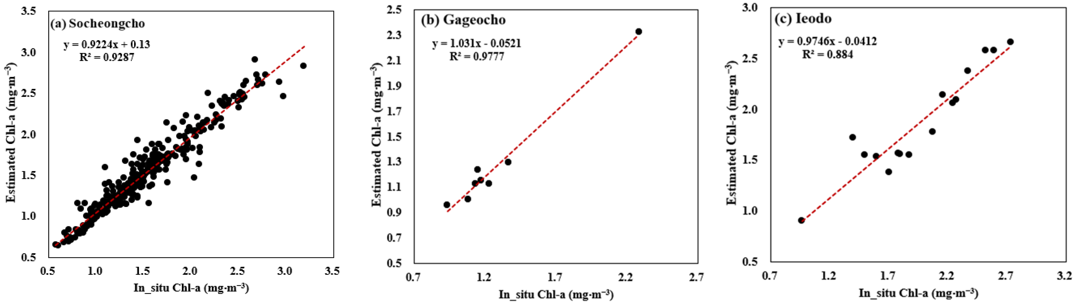
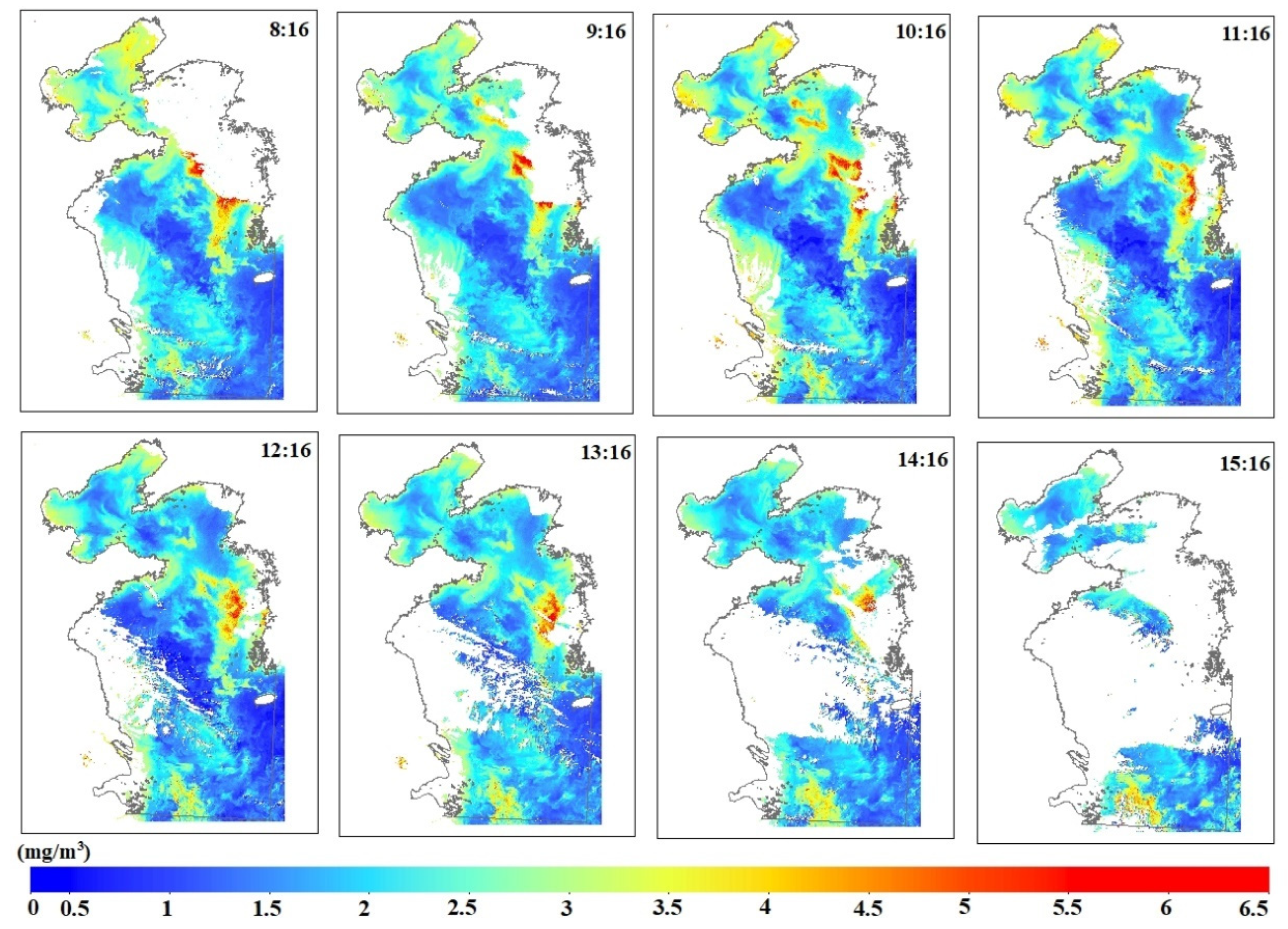
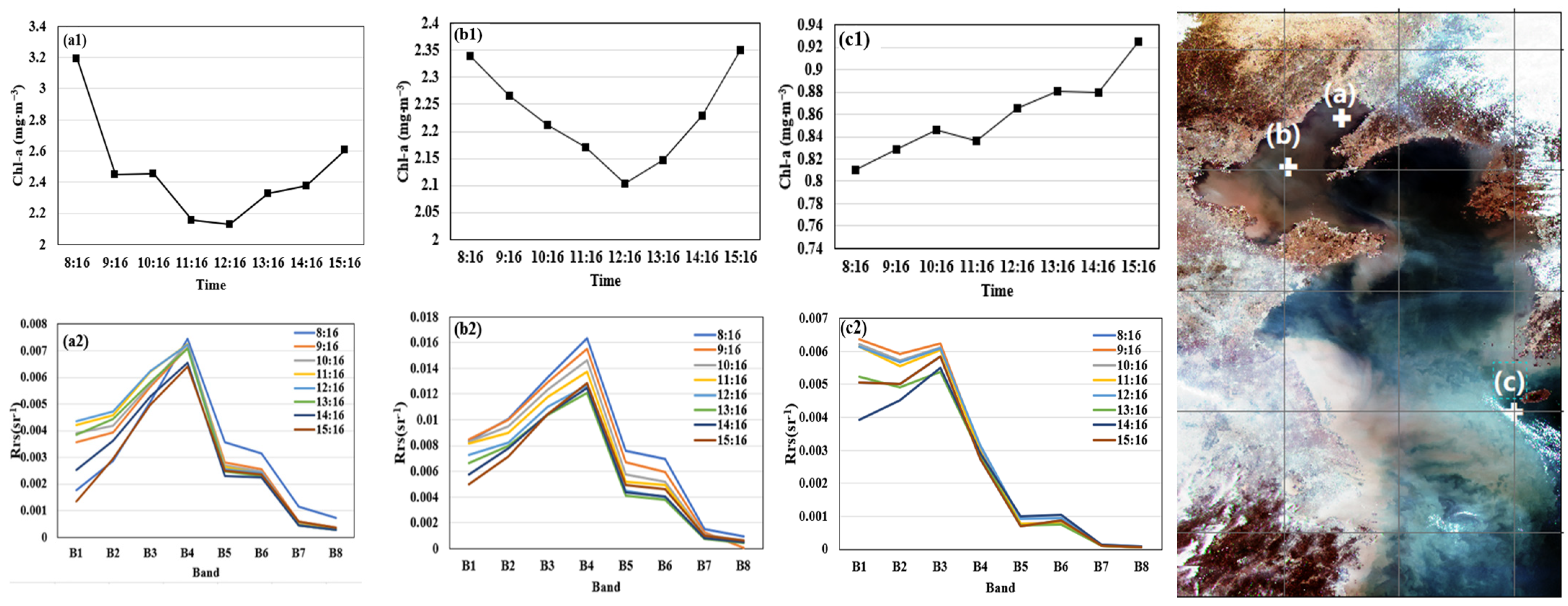
3.2.2. Details of Diurnal Variation Change in Chl-a

GOCI’s daily 8-view images with an hourly temporal resolution provide the ability to analyze the diurnal variation in chlorophyll concentration in the study area. This study presents a case study that examines the diurnal variation in the Chl-a at eight different times on 15 April 2019. The retrieval results are displayed in Figure 9.

Phytoplankton show circadian rhythmicity in response to environmental factors like water temperature and light, leading to vertical movements within the water column. Under ideal weather conditions, seawater and algal motion can modify sensor-reflected signals, facilitating remote monitoring of the horizontal and vertical displacement changes in cyanobacteria. Three representative sites within the study area were selected to assess GOCI’s ability to monitor intraday variations in chlorophyll concentration, as shown in Figure 10. The findings suggest that the first two sites display high levels of chlorophyll in the morning, which decreases by noon and reaches the lowest level at around 12:00 a.m. On the other hand, the third site shows a gradual increase in chlorophyll concentration from morning to evening. We also plot the spectra for the considered time points in Figure 10. Since there is no actual measurement for monitoring diurnal variation, further validation is necessary to demonstrate the ability of the proposed model to accurately reflect changes in chlorophyll concentration. Nevertheless, the results demonstrate GOCI’s capability in capturing diurnal chlorophyll variations, which indicates a potential approach for real-time red tide monitoring.

4. Discussion

4.1. Necessity and Limitations of GOCI Reflectance Correction

Our investigation focused on the Bohai–Yellow Sea region, particularly the Bohai Sea, which has drawn considerable attention due to water environment eutrophication caused by rapid urban development of neighboring cities. Satellite remote sensing has emerged as a favored research field for acquiring spatial and temporal information on water quality rapidly and at a low cost [59].

In this regard, we turned to the Geostationary Ocean Color Imager (GOCI) aboard geostationary satellites. GOCI offers continuous observation of marine hazards, rendering it especially effective for satellite remote sensing [41]. However, the accuracy of GOCI’s water color products, including $R_{rs}\left(\lambda \right)$ and Chl-a, is limited in the Bohai–Yellow Sea region due to the complex optical characteristics of Case II water bodies. The presence of constituents such as chlorophyll, CDOM, and SPM leads to varying spectral characteristics [60]. Variations in Chl-a result in distinct differences in the 400–700 nm band, forming the basis for remote sensing inversion [61]. Therefore, it is necessary to ensure accurate spectral information for building the inversion model. Additionally, we have evaluated and corrected GOCI’s reflectance products using data from the AERONET-OC, and the results have demonstrated the necessity and feasibility of the proposed correction model in obtaining reliable GOCI reflectance evaluated by in situ measured data with an R² higher than 0.9. However, due to the limited number of AERONET-OC stations in the Bohai–Yellow Sea region and varying amounts of long-duration data provided by each station, the data’s representativeness for the entire study area is restricted. Therefore, obtaining additional measured spectral data for the entire study area to increase data volume and enhance spatial representativeness is necessary in future studies.

4.2. Feasibility and Limitations of the Constructed Chl-a Inversion Model

Using corrected GOCI reflectance, we evaluated empirical algorithms (OC4, OC5, YOC) and machine learning methods to invert Chl-a in the Bohai–Yellow Sea. The results indicate that the machine learning models exhibit promising accuracy and robustness in predicting Chl-a in the Bohai–Yellow Sea. Moreover, when compared to empirical models, the machine learning approaches demonstrate clear advantages in capturing complex nonlinear relationships within the data. Among all selected machine learning methods, random forest (RF) performs the best (R² of 0.916, RMSE of 0.212 mg$·$m⁻³, and MAPE of 14.27%). Being an ensemble model, it can achieve higher prediction accuracy than individual learners [50]. The successful inversion of Chl-a in the Bohai–Yellow Sea using the RF method holds significant implications for the monitoring and management of the region’s ecological environment. Timely access to spatial chlorophyll concentration information enhances understanding of the Bohai–Yellow Sea’s ecosystem health and trends, supporting informed decision-making.

However, despite the favorable performance of machine learning methods in Chl-a inversion, it is crucial to recognize their limitations. Firstly, the quality and representativeness of training data significantly impact the effectiveness of machine learning models. Additionally, outliers and noise within data can undermine the models’ performance. Without adequate and unbiased training data, these models may fail to make accurate predictions. Moreover, machine learning models frequently operate as black-box models, posing difficulties in interpreting their internal mechanisms and decision-making processes, consequently restricting our grasp and interpretive ability regarding the model’s predictions [62].

In addition to the inherent disadvantages of machine learning, this work only covers the study area of the Bohai–Yellow Sea; further discussion of its applicability to other sea areas is required. Since impurities and turbidity vary between regions, more in situ data should be collected when the proposed model application is expanded from the Bohai–Yellow Sea to other sea areas.

4.3. Reliability of Temporal Changes in Estimated Chl-a

Based on the established RF model, we inverted the long time series Chl-a, showcasing its feasibility for long-term monitoring in the Bohai–Yellow Sea. There are significant seasonal Chl-a changes in the Bohai–Yellow Sea. In the Bohai–Yellow Sea offshore region, Chl-a values are significantly higher in winter and spring than in summer and autumn, and this is consistent with [63]. However, in the Yellow Sea coastal region, Chl-a peaks in the summer. The seasonal pattern in the Yellow Sea is similar to that in a previous study [64,65]. As a temperate continental shelf marine ecosystem, the Chl-a dynamics of the Bohai–Yellow Sea reflect a tight balance between nutrient supply and light availability [65]. The high Chl-a during winter can be explained by strong winter winds and lower SST that enhance vertical mixing and nutrients from subsurface layers brought to the euphotic layer. However, there exist some differences such as reported by Qian [66], indicating that in coastal regions where the Chl-a peak coincides with the emergent summer monsoon over eastern China, and by Hyun [67], indicating that in offshore regions, a strong spring bloom occurs. We speculate that these differences are likely caused by the utility of different datasets and different time spans of data used in building the inversion model.

Moreover, to comprehend the diurnal pattern of Chl-a, further investigation is required due to the lack of measured data at eight specific moments of the day and regional variations. Furthermore, the data’s validity is affected by the presence of clouds, which can also influence the statistical results.

5. Conclusions

In this paper, three empirical algorithms and four machine learning methods were used to build an inverse model of chlorophyll concentration in the Bohai–Yellow Sea using GOCI data, and the accuracy of the model was evaluated to select the most suitable Chl-a inversion model. The spatial, seasonal, and diurnal variations in Chl-a in the Bohai Sea were retrieved by the selected RF retrieval model. Through comparison and analysis, the main findings are as follows:

(1)

The proposed correction model can obtain reliable GOCI reflectance evaluated by in situ measured data with R² values higher than 0.9.

(2)

Compared with traditional empirical methods, machine learning can better establish the non-linear relationship between data. The random forest method performs the best and has the highest inversion accuracy (R² of 0.916, RMSE of 0.212 mg$·$m⁻³, and MAPE of 14.27%).

(3)

Chl-a displays a discernible spatial pattern in the Bohai–Yellow Sea, with a significant decline in concentration from nearshore to offshore regions. This particular distribution could potentially be linked to the high levels of nutrients flowing into the nearshore through land-based rivers alongside the shallow water that promotes more robust growth of algal flora.

(4)

The analysis of the seasonal Chl-a pattern in the Bohai–Yellow Sea during 2019 reveals significant changes linked to the seasons. The inversion results show that Chl-a is considerably higher in winter and spring compared to autumn and summer. Diurnal variation retrieval effectively demonstrates GOCI’s potential as a capable tool for monitoring intraday changes in chlorophyll-a concentrations.

The GOCI reflectance correction is a crucial step in the retrieval of Chl-a. Additional spectral data over the entire study area are essential for achieving spatial representativeness. Machine learning techniques outperform empirical algorithms in Chl-a inversion. Future studies will focus on expanding the proposed models’ application to other sea areas to verify their stability and accuracy and exploring the potential of alternative machine learning techniques for this problem.

References

1. Brooks, B.W.; Lazorchak, J.M.; Howard, M.D.; Johnson, M.V.; Morton, S.L.; Perkins, D.A.; Reavie, E.D.; Scott, G.I.; Smith, S.A.; Steevens, J.A. Are harmful algal blooms becoming the greatest inland water quality threat to public health and aquatic ecosystems? Environ. Toxicol. Chem. 2016, 35, 6–13. [Google Scholar] [CrossRef] [PubMed]
2. Laliberte, J.; Larouche, P. Chlorophyll-a concentration climatology, phenology, and trends in the optically complex waters of the St. Lawrence Estuary and Gulf. J. Mar. Syst. 2023, 238, 103830. [Google Scholar] [CrossRef]
3. Batur, E.; Maktav, D. Assessment of Surface Water Quality by Using Satellite Images Fusion Based on PCA Method in the Lake Gala, Turkey. IEEE Trans. Geosci. Remote Sens. 2019, 57, 2983–2989. [Google Scholar] [CrossRef]
4. Gordon, H.R.; Clark, D.K.; Brown, J.W.; Brown, O.B.; Evans, R.H.; Broenkow, W.W. Phytoplankton pigment concentrations in the middle atlantic bight—Comparison of ship determinations and czcs estimates. Appl. Opt. 1983, 22, 20–36. [Google Scholar] [CrossRef] [PubMed]
5. Yoder, J.A.; McClain, C.R.; Feldman, G.C.; Esaias, W.E. Annual cycles of phytoplankton chlorophyll concentrations in the global ocean—A satellite view. Glob. Biogeochem. Cycles 1993, 7, 181–193. [Google Scholar] [CrossRef]
6. Pahlevan, N.; Smith, B.; Schalles, J.; Binding, C.; Cao, Z.; Ma, R.; Alikas, K.; Kangro, K.; Gurlin, D.; Hà, N.; et al. Seamless retrievals of chlorophyll-a from Sentinel-2 (MSI) and Sentinel-3 (OLCI) in inland and coastal waters: A machine-learning approach. Remote Sens. Environ. 2020, 240, 111604. [Google Scholar] [CrossRef]
7. Yang, Y.; Zhang, X.; Gao, W.; Zhang, Y.; Hou, X. Improving lake chlorophyll-a interpreting accuracy by combining spectral and texture features of remote sensing. Environ. Sci. Pollut. Res. Int. 2023, 30, 83628–83642. [Google Scholar] [CrossRef]
8. Gitelson, A.A.; Dall’Olmo, G.; Moses, W.; Rundquist, D.C.; Barrow, T.; Fisher, T.R.; Gurlin, D.; Holz, J. A simple semi-analytical model for remote estimation of chlorophyll-a in turbid waters: Validation. Remote Sens. Environ. 2008, 112, 3582–3593. [Google Scholar] [CrossRef]
9. O’Reilly, J.E.; Maritorena, S.; Mitchell, B.G.; Siegel, D.A.; Carder, K.L.; Garver, S.A.; Kahru, M.; McClain, C. Ocean color chlorophyll algorithms for SeaWiFS. J. Geophys. Res. Ocean. 1998, 103, 24937–24953. [Google Scholar] [CrossRef]
10. O’Reilly, J.E.; Werdell, P.J. Chlorophyll Algorithms for Ocean Color Sensors—Oc4, Oc5 & Oc6. Remote Sens. Environ. 2019, 229, 32–47. [Google Scholar] [CrossRef]
11. Hu, C.; Feng, L.; Lee, Z.; Franz, B.A.; Bailey, S.W.; Werdell, P.J.; Proctor, C.W. Improving Satellite Global Chlorophyll a Data Products Through Algorithm Refinement and Data Recovery. J. Geophys. Res. Ocean. 2019, 124, 1524–1543. [Google Scholar] [CrossRef]
12. Hu, C.; Lee, Z.; Franz, B. Chlorophyll a algorithms for oligotrophic oceans: A novel approach based on three-band reflectance difference. J. Geophys. Res. Ocean. 2012, 117, C01011. [Google Scholar] [CrossRef]
13. Rodriguez-Lopez, L.; Duran-Llacer, I.; Gonzalez-Rodriguez, L.; Abarca-del-Rio, R.; Cardenas, R.; Parra, O.; Martinez-Retureta, R.; Urrutia, R. Spectral analysis using LANDSAT images to monitor the chlorophyll-a concentration in Lake Laja in Chile. Ecol. Inform. 2020, 60, 101183. [Google Scholar] [CrossRef]
14. Wang, X.; Gong, Z.; Pu, R. Estimation of chlorophyll a content in inland turbidity waters using WorldView-2 imagery: A case study of the Guanting Reservoir, Beijing, China. Environ. Monit. Assess. 2018, 190, 620. [Google Scholar] [CrossRef] [PubMed]
15. Fu, L.; Zhou, Y.; Liu, G.; Song, K.; Tao, H.; Zhao, F.; Li, S.; Shi, S.; Shang, Y. Retrieval of Chla Concentrations in Lake Xingkai Using OLCI Images. Remote Sens. 2023, 15, 3809. [Google Scholar] [CrossRef]
16. Cao, Z.; Ma, R.; Duan, H.; Pahlevan, N.; Melack, J.; Shen, M.; Xue, K. A machine learning approach to estimate chlorophyll-a from Landsat-8 measurements in inland lakes. Remote Sens. Environ. 2020, 248, 111974. [Google Scholar] [CrossRef]
17. Guo, H.; Tian, S.; Huang, J.J.; Zhu, X.; Wang, B.; Zhang, Z. Performance of deep learning in mapping water quality of Lake Simcoe with long-term Landsat archive. ISPRS J. Photogramm. Remote Sens. 2022, 183, 451–469. [Google Scholar] [CrossRef]
18. Cao, Z.; Ma, R.; Duan, H.; Xue, K. Effects of broad bandwidth on the remote sensing of inland waters: Implications for high spatial resolution satellite data applications. ISPRS J. Photogramm. Remote Sens. 2019, 153, 110–122. [Google Scholar] [CrossRef]
19. Pyo, J.; Duan, H.; Baek, S.; Kim, M.S.; Jeon, T.; Kwon, Y.S.; Lee, H.; Cho, K.H. A convolutional neural network regression for quantifying cyanobacteria using hyperspectral imagery. Remote Sens. Environ. 2019, 233, 111350. [Google Scholar] [CrossRef]
20. Chen, Z.; Dou, M.; Xia, R.; Li, G.; Shen, L. Spatiotemporal evolution of chlorophyll-a concentration from MODIS data inversion in the middle and lower reaches of the Hanjiang River, China. Environ. Sci. Pollut. Res. 2022, 29, 38143–38160. [Google Scholar] [CrossRef]
21. Chen, S.; Hu, C.; Barnes, B.B.; Wanninkhof, R.; Cai, W.-J.; Barbero, L.; Pierrot, D. A machine learning approach to estimate surface ocean pCO(2) from satellite measurements. Remote Sens. Environ. 2019, 228, 203–226. [Google Scholar] [CrossRef]
22. Werther, M.; Odermatt, D.; Simis, S.G.H.; Gurlin, D.; Lehmann, M.K.; Kutser, T.; Gupana, R.; Varley, A.; Hunter, P.D.; Tyler, A.N.; et al. A Bayesian approach for remote sensing of chlorophyll-a and associated retrieval uncertainty in oligotrophic and mesotrophic lakes. Remote Sens. Environ. 2022, 283, 113295. [Google Scholar] [CrossRef]
23. Cui, T.W.; Zhang, J.; Wang, K.; Wei, J.W.; Mu, B.; Ma, Y.; Zhu, J.H.; Liu, R.J.; Chen, X.Y. Remote sensing of chlorophyll a concentration in turbid coastal waters based on a global optical water classification system. ISPRS J. Photogramm. Remote Sens. 2020, 163, 187–201. [Google Scholar] [CrossRef]
24. Li, J.; Gao, M.; Feng, L.; Zhao, H.; Shen, Q.; Zhang, F.; Wang, S.; Zhang, B. Estimation of Chlorophyll-a Concentrations in a Highly Turbid Eutrophic Lake Using a Classification-Based MODIS Land-Band Algorithm. IEEE J. Sel. Top. Appl. Earth Obs. Remote Sens. 2019, 12, 3769–3783. [Google Scholar] [CrossRef]
25. Zhang, S.; Zhu, H.; Li, J.; Yang, Y.; Liu, H. Data-Free Area Detection and Evaluation for Marine Satellite Data Products. Remote Sens. 2022, 14, 3815. [Google Scholar] [CrossRef]
26. Chen, S.; Hu, C.; Barnes, B.B.; Xie, Y.; Lin, G.; Qiu, Z. Improving ocean color data coverage through machine learning. Remote Sens. Environ. 2019, 222, 286–302. [Google Scholar] [CrossRef]
27. Harvey, E.T.; Kratzer, S.; Philipson, P. Satellite-based water quality monitoring for improved spatial and temporal retrieval of chlorophyll-a in coastal waters. Remote Sens. Environ. 2015, 158, 417–430. [Google Scholar] [CrossRef]
28. Kim, Y.W.; Kim, T.; Shin, J.; Lee, D.-S.; Park, Y.-S.; Kim, Y.; Cha, Y. Validity evaluation of a machine-learning model for chlorophyll a retrieval using Sentinel-2 from inland and coastal waters. Ecol. Indic. 2022, 137, 108737. [Google Scholar] [CrossRef]
29. Zhu, X.; Guo, H.; Huang, J.J.; Tian, S.; Xu, W.; Mai, Y. An ensemble machine learning model for water quality estimation in coastal area based on remote sensing imagery. J. Environ. Manag. 2022, 323, 116187. [Google Scholar] [CrossRef]
30. Chen, B.; Mu, X.; Chen, P.; Wang, B.; Choi, J.; Park, H.; Xu, S.; Wu, Y.; Yang, H. Machine learning-based inversion of water quality parameters in typical reach of the urban river by UAV multispectral data. Ecol. Indic. 2021, 133, 108434. [Google Scholar] [CrossRef]
31. Fan, Y.; Li, S.; Han, X.; Stamnes, K. Machine learning algorithms for retrievals of aerosol and ocean color products from FY-3D MERSI-II instrument. J. Quant. Spectrosc. Radiat. Transf. 2020, 250, 107042. [Google Scholar] [CrossRef]
32. Guo, J.; Liu, X.; Xie, Q. Characteristics of the Bohai Sea oil spill and its impact on the Bohai Sea ecosystem. Chin. Sci. Bull. 2013, 58, 2276–2281. [Google Scholar] [CrossRef]
33. Li, Y.; He, R. Spatial and temporal variability of SST and ocean color in the Gulf of Maine based on cloud-free SST and chlorophyll reconstructions in 2003–2012. Remote Sens. Environ. 2014, 144, 98–108. [Google Scholar] [CrossRef]
34. Zhang, M.; Tang, J.; Song, Q.; Dong, Q. Backscattering ratio variation and its implications for studying particle composition: A case study in Yellow and East China seas. J. Geophys. Res. Ocean. 2010, 115, C12014. [Google Scholar] [CrossRef]
35. Ji, C.; Zhang, Y.; Cheng, Q.; Tsou, J.; Jiang, T.; Liang, X.S. Evaluating the impact of sea surface temperature (SST) on spatial distribution of chlorophyll-a concentration in the East China Sea. Int. J. Appl. Earth Obs. Geoinf. 2018, 68, 252–261. [Google Scholar] [CrossRef]
36. Shi, W.; Wang, M.H. Satellite views of the Bohai Sea, Yellow Sea, and East China Sea. Prog. Oceanogr. 2012, 104, 30–45. [Google Scholar] [CrossRef]
37. Berthon, J.-F.; Mélin, F.; Zibordi, G.; Holben, B.; Slutsker, I.; Giles, D.; D’Alimonte, D.; Vandemark, D.; Feng, H.; Schuster, G.; et al. AERONET-OC: A Network for the Validation of Ocean Color Primary Products. J. Atmos. Ocean. Technol. 2009, 26, 1634–1651. [Google Scholar] [CrossRef]
38. Xu, Y.; He, X.; Bai, Y.; Zhu, Q.; Gong, F. Validations of the HY-1C COCTS remote sensing reflectance products in coastal waters. J. Remote Sens. 2023, 27, 14–25. [Google Scholar] [CrossRef]
39. Zibordi, G.; Holben, B.N.; Talone, M.; D’Alimonte, D.; Slutsker, I.; Giles, D.M.; Sorokin, M.G. Advances in the Ocean Color Component of the Aerosol Robotic Network (AERONET-OC). J. Atmos. Ocean. Technol. 2021, 38, 725–746. [Google Scholar] [CrossRef]
40. Lawson, A.; Bowers, J.; Ladner, S.; Crout, R.; Wood, C.; Arnone, R.; Martinolich, P.; Lewis, D. Analyzing Satellite Ocean Color Match-Up Protocols Using the Satellite Validation Navy Tool (SAVANT) at MOBY and Two AERONET-OC Sites. Remote Sens. 2021, 13, 2673. [Google Scholar] [CrossRef]
41. Ryu, J.-H.; Han, H.-J.; Cho, S.; Park, Y.-J.; Ahn, Y.-H. Overview of geostationary ocean color imager (GOCI) and GOCI data processing system (GDPS). Ocean. Sci. J. 2012, 47, 223–233. [Google Scholar] [CrossRef]
42. Sun, L.; Wang, X.; Guo, M.; Tang, J. MODIS ocean color product validation around the Yellow Sea and East China Sea. J. Lake Sci. 2009, 21, 298–306. [Google Scholar]
43. Ahmed, S.; Gilerson, A.; Hlaing, S.; Ioannou, I.; Wang, M.; Weidemann, A.; Arnone, R. Evaluation of VIIRS Ocean Color Data Using Measurements from the AERONET-OC Sites; SPIE: Bellingham, WA, USA, 2013; Volume 8724. [Google Scholar]
44. Moon, J.-E.; Park, Y.-J.; Ryu, J.-H.; Choi, J.-K.; Ahn, J.-H.; Min, J.-E.; Son, Y.-B.; Lee, S.-J.; Han, H.-J.; Ahn, Y.-H. Initial validation of GOCI water products against in situ data collected around Korean peninsula for 2010–2011. Ocean Sci. J. 2012, 47, 261–277. [Google Scholar] [CrossRef]
45. Tassan, S. Local algorithms using seawifs data for the retrieval of phytoplankton, pigments, suspended sediment, and yellow substance in coastal waters. Appl. Opt. 1994, 33, 2369–2378. [Google Scholar] [CrossRef] [PubMed]
46. Siswanto, E.; Tang, J.; Yamaguchi, H.; Ahn, Y.-H.; Ishizaka, J.; Yoo, S.; Kim, S.-W.; Kiyomoto, Y.; Yamada, K.; Chiang, C.; et al. Empirical ocean-color algorithms to retrieve chlorophyll-a, total suspended matter, and colored dissolved organic matter absorption coefficient in the Yellow and East China Seas. J. Oceanogr. 2011, 67, 627–650. [Google Scholar] [CrossRef]
47. Dou, P.; Chen, Y.; Yue, H. Remote-sensing imagery classification using multiple classification algorithm-based AdaBoost. Int. J. Remote Sens. 2018, 39, 619–639. [Google Scholar] [CrossRef]
48. Reulen, H.; Kneib, T. Boosting multi-state models. Lifetime Data Anal. 2016, 22, 241–262. [Google Scholar] [CrossRef]
49. Breiman, L. Random Forests. Mach. Learn. 2001, 45, 5–32. [Google Scholar] [CrossRef]
50. Belgiu, M.; Drăguţ, L. Random forest in remote sensing: A review of applications and future directions. ISPRS J. Photogramm. Remote Sens. 2016, 114, 24–31. [Google Scholar] [CrossRef]
51. Palani, S.; Liong, S.Y.; Tkalich, P.; Palanichamy, J. Development of a neural network model for dissolved oxygen in seawater. Indian J. Mar. Sci. 2009, 38, 151–159. [Google Scholar]
52. Chang, C.-C.; Lin, C.-J. LIBSVM: A Library for Support Vector Machines. ACM Trans. Intell. Syst. Technol. 2011, 2, 1–27. [Google Scholar] [CrossRef]
53. Barbosa dos Santos, V.; Moreno Ferreira dos Santos, A.; da Silva Cabral de Moraes, J.R.; de Oliveira Vieira, I.C.; de Souza Rolim, G. Machine learning algorithms for soybean yield forecasting in the Brazilian Cerrado. J. Sci. Food Agric. 2022, 102, 3665–3672. [Google Scholar] [CrossRef] [PubMed]
54. Marabel, M.; Alvarez-Taboada, F. Spectroscopic Determination of Aboveground Biomass in Grasslands Using Spectral Transformations, Support Vector Machine and Partial Least Squares Regression. Sensors 2013, 13, 10027–10051. [Google Scholar] [CrossRef] [PubMed]
55. Seegers, B.N.; Stumpf, R.P.; Schaeffer, B.A.; Loftin, K.A.; Werdell, P.J. Performance metrics for the assessment of satellite data products: An ocean color case study. Opt. Express 2018, 26, 7404–7422. [Google Scholar] [CrossRef]
56. Wang, M.; Cheng, Y.; Long, X.; Yang, B. On-orbit geometric calibration approach for high-resolution geostationary optical satellite GaoFen-4. In Proceedings of the XXIII ISPRS Congress, Commission I, Prague, Czech Republic, 12–19 July 2016; pp. 389–394. [Google Scholar]
57. Cai, L.; Bu, J.; Tang, D.; Zhou, M.; Yao, R.; Huang, S. Geosynchronous Satellite GF-4 Observations of Chlorophyll-a Distribution Details in the Bohai Sea, China. Sensors 2020, 20, 5471. [Google Scholar] [CrossRef]
58. Park, J.-E.; Park, K.-A. Application of Deep Learning for Speckle Removal in GOCI Chlorophyll-a Concentration Images (2012–2017). Remote Sens. 2021, 13, 585. [Google Scholar] [CrossRef]
59. Cai, L.; Yu, M.; Yan, X.; Zhou, Y.; Chen, S. HY-1C/D Reveals the Chlorophyll-a Concentration Distribution Details in the Intensive Islands’ Waters and Its Consistency with the Distribution of Fish Spawning Ground. Remote Sens. 2022, 14, 4270. [Google Scholar] [CrossRef]
60. Al Shehhi, M.R.; Gherboudj, I.; Zhao, J.; Ghedira, H. Improved atmospheric correction and chlorophyll-a remote sensing models for turbid waters in a dusty environment. ISPRS J. Photogramm. Remote Sens. 2017, 133, 46–60. [Google Scholar] [CrossRef]
61. Liu, G.; Li, L.; Song, K.; Li, Y.; Lyu, H.; Wen, Z.; Fang, C.; Bi, S.; Sun, X.; Wang, Z.; et al. An OLCI-based algorithm for semi-empirically partitioning absorption coefficient and estimating chlorophyll a concentration in various turbid case-2 waters. Remote Sens. Environ. 2020, 239, 111648. [Google Scholar] [CrossRef]
62. Silveira Kupssinsku, L.; Thomassim Guimaraes, T.; Menezes de Souza, E.; Zanotta, D.C.; Roberto Veronez, M.; Gonzaga, L., Jr.; Mauad, F.F. A Method for Chlorophyll-a and Suspended Solids Prediction through Remote Sensing and Machine Learning. Sensors 2020, 20, 2125. [Google Scholar] [CrossRef]
63. Li, Q.; Wen-ling, L.; Xiao-shen, Z. Spatial-temporal variation of Chlorophyll-a concentration in Bohai Sea based on MODIS. Main Escience Bull. 2011, 30, 683–687. [Google Scholar]
64. Zhang, K.; Zhao, X.; Xue, J.; Mo, D.; Zhang, D.; Xiao, Z.; Yang, W.; Wu, Y.; Chen, Y. The temporal and spatial variation of chlorophyll a concentration in the China Seas and its impact on marine fisheries. Front. Mar. Sci. 2023, 10, 1212992. [Google Scholar] [CrossRef]
65. Wang, Y.; Liu, D.; Wang, Y.; Gao, Z.; Keesing, J.K. Evaluation of standard and regional satellite chlorophyll-a algorithms for moderate-resolution imaging spectroradiometer (MODIS) in the Bohai and Yellow Seas, China: A comparison of chlorophyll-a magnitude and seasonality. Int. J. Remote Sens. 2019, 40, 4980–4995. [Google Scholar] [CrossRef]
66. Qian, W.; Kang, H.S.; Lee, D.K. Distribution of seasonal rainfall in the East Asian monsoon region. Theor. Appl. Climatol. 2002, 73, 151–168. [Google Scholar] [CrossRef]
67. Hyun, J.H.; Kim, K.H. Bacterial abundance and production during the unique spring phytoplankton bloom in the central Yellow Sea. Mar. Ecol. Prog. Ser. 2003, 252, 77–88. [Google Scholar] [CrossRef]
Figure 1. Location of sample points including AERONET-OC and collected in situ Chl-a. Annotated on the image are the locations of the sampling points: AERONET-OC (which is used for GOCI spectral remote sensing reflectance correction and Chl-a retrieval), other Chl-a points measured in 2012 and 2017 (only used for Chl-a retrieval).
Remotesensing 15 05285 g001
Figure 2. The flowchart of Chl-a retrieval modeling.
Remotesensing 15 05285 g002
Figure 3. Compariation of the corrected GOCI  R r s λ  products against AERONET-OC field measurements: (af) represent scatter plots of the six bands before and after correction, Green squares mean before correction, and blue dots represent after correction (the number of scatter dots in each color N = 360).
Remotesensing 15 05285 g003
Figure 4. Boxplot representing the R2 metric obtained on cross-validation; the mean value is marked with a diamond.
Remotesensing 15 05285 g004
Figure 5. Scatter verification of Chl-a values estimated from four models and measured values, the x-coordinate is in situ Chl-a, and the y-coordinate is model estimated Chl-a, both in units of mg · m−3, (a) Random forest. (b) SVR. (c) BPNN. (d) AdaBoost.
Remotesensing 15 05285 g005aRemotesensing 15 05285 g005b
Figure 6. Comparison of in situ and GOCI estimated Chl-a for three AERONET-OC stations: (a) Socheongcho station; (b) Gageocho station; and (c) Ieodo station.
Remotesensing 15 05285 g006
Figure 7. January–December 2019 spatial distribution of monthly mean Chl-a estimated from GOCI using the RF model.
Remotesensing 15 05285 g007
Figure 8. The histogram distributions of GOCI-estimated Chl-a for different seasons during 2019.
Remotesensing 15 05285 g008
Figure 9. Spatial distribution of Chl-a at eight moments estimated from GOCI on 15 April 2019.
Remotesensing 15 05285 g009
Figure 10. Diurnal variation curves of chlorophyll concentration and  R r s λ  at three typical sites on 15 April 2019. (ac) represent three randomly selected typical sites, (a1c1) are the Chl-a diurnal variation for the corresponding sites, and (a2c2) represent the spectral curves at the corresponding time for each site.
Remotesensing 15 05285 g010