

Coastal Assessment of Sentinel-6 Altimetry Data during the Tandem Phase with Jason-3

Deutsches Geodätisches Forschungsinstitut der Technischen Universität München (DGFI-TUM), Arcisstraße 21, 80333 Munich, Germany
*
Author to whom correspondence should be addressed.
Remote Sens. 2023, 15(17), 4161; https://0-doi-org.brum.beds.ac.uk/10.3390/rs15174161
Submission received: 14 July 2023
/
Revised: 21 August 2023
/
Accepted: 22 August 2023
/
Published: 24 August 2023
(This article belongs to the Special Issue Validation and Evaluation of Global Ocean Satellite Products)
Abstract
:This study presents a comparative analysis of the coastal performances of Sentinel-6 and Jason-3 altimeters during their tandem phase, considering their different processing modes. We examine the measurements available in the standard geophysical data records (GDR) and also perform dedicated reprocessing using coastal retracking algorithms applied to the original waveforms. The performances are evaluated, taking into account the quality of retrievals (outlier analysis), their precision (along-track noise analysis), potential systematic biases, and accuracy (comparison against tide gauges). The official SAR altimetry product of Sentinel-6 demonstrates improved coastal monitoring capabilities compared to Jason-3, except for the remaining issues related to significant wave height, which have already been identified. These findings highlight the significance of dedicated coastal retracking algorithms for enhancing the capabilities of both traditional, pulse-limited altimeters and more recent developments utilizing SAR altimetry.
1. Introduction
The monitoring of coastal sea level from space is increasingly possible through satellite altimetry, which is based on the measurement of the two-way travel time that radar pulses employ from transmission towards the ocean surface to reception [1]. Indeed, the improvement of coastal altimetry performance is one of the expected results of the latest generation of altimeters: the SAR altimeters based on the delay-Doppler principle [2].
Traditional altimeters, nowadays identified as low-resolution mode (LR), are characterized by a limit in the number of pulses per second (the pulse repetition frequency). The independent pulses are averaged on board over a certain along-track length (typically about 300 m, corresponding to a 20 Hz posting rate) to reduce the noise. The SAR processing exploits a higher pulse repetition frequency than traditional altimeters, with the objective of achieving phase coherence within consecutively transmitted pulses. All these individual pulses are downlinked to ground. In this way, multiple views of the same illuminated area (beam, also typically designed with a 20 Hz posting rate) can be collected at slightly different viewing angles, identified by the Doppler shift due to the satellite movement with respect to the ocean surface [3]. These views are incoherently averaged, creating a so-called “multi-looked” waveform, which has a better signal-to-noise ratio and a smaller along-track footprint than its LR counterpart [4].
Sentinel-6 Michael Freilich (S6) was launched on 21 November 2020 as the successor to Jason-3 (J3). It uses the same orbit and some instrumental heritage; however, it carries an SAR altimeter operating in an open-burst measuring approach, meaning that the radar chronogram is interleaved such that the pulses are transmitted and received in an interleaved manner [5]. This allows for a direct comparison between SAR and LR data. Moreover, during the first months of the mission, S6 flew in tandem with J3 and took measurements just 30 s apart. This enables further comparison possibilities between S6 and J3.
Besides the technological improvements, the coastal performance of altimetry relies on two other pillars. Firstly, there is a dedicated fitting of the waveforms, called retracking, in order to avoid spurious interference from areas characterized by different backscattering characteristics (for example, land or calm water patches due to sheltering) within the footprint [6]. Secondly, a set of geophysical adjustments and corrections that avoid further coastal issues, such as the fact that the delay due to the presence of water vapor in the atmosphere, may be computed using a radiometer onboard the satellite receiving spurious signals from land when approaching the coast [7]. In the last decade, studies have demonstrated that LR altimetry with specific coastal reprocessing and proper data screening can deliver accurate measurements even closer than 3 km from the coast [8,9], with enough quality to be used for sea level trend studies [10,11,12]. At the same time, it has been shown that dedicated coastal processing can significantly enhance the coastal performance of SAR altimeters [13,14].
The objective of this work is to assess the quality and the quantity of sea level measurements in the coastal zone using both standard data and dedicated reprocessing for SAR and LR waveforms during the tandem mission of S6 and J3. For the first time, the latest developments in coastal altimetry can be compared for different altimeters spanning the same tracks at almost the same time. The performance is analyzed using metrics inherited from previous literature in order to guarantee the objectiveness of the analysis. We focus on the quantity of retrievals (outlier analysis), their precision (along-track noise analysis), potential systematic differences (bias analysis), and their accuracy (comparison against in situ data).
2. Data
The study uses all available data on coastal areas on a global scale. The data extraction was accomplished based on the distance to the coast, up to a threshold of 100 km. No further criteria for data exclusion were applied; i.e., data in estuaries or sea ice areas are also included in the analyses. For the analyses in Section 4.2, latitudes above/below 40 degrees (north/south) have also been excluded.
2.1. General Characteristics
We use cycles 13 to 22 for S6, corresponding to cycles 188 to 197 for J3. The limitation in the number of cycles was necessary to allow for a full reprocessing with several different retrackers on a common baseline and in time with the evaluation of the project “Sentinel-6 Michael Freilich and Jason-3 tandem Flight Exploitation (S6-JTEX)” from the European Space Agency, in the context of which this study has been performed (see Acknowledgments). In particular, we consider Level 1B data, which contain all necessary parameters for retracking and include waveforms, and Level 2 data, which contain retracked parameters such as range and significant wave height (SWH), as well as all necessary geophysical adjustments and corrections to compute the sea level anomaly (SLA). The latter is computed as follows:
where SSB is the sea state bias correction [15], and DAC is the dynamic atmospheric correction. A complete description of the different geophysical adjustments and corrections can be found in [16]. The atmospheric corrections (dry and wet troposphere and ionosphere) can be derived from models or measured directly on board the satellite, either by the altimeter itself (in the case of the ionosphere) or by a microwave radiometer (in the case of the wet troposphere). For the purpose of this work, we utilize the first source, which is recommended for the coastal environment [17]. Each retracker analyzed in this work has its specific range and SSB output, unless otherwise stated. Moreover, we have taken into account their respective quality flags.
2.2. Retracked Ranges from the Original Data
We use original data from S6 in its F06 processing baseline and from J3 in its Geophysical Data Record, version F (GDR-F) processing baseline. These were the latest releases at the start of the analysis (July 2022); therefore, any further update is outside the scope of this study.
The original S6 ranges in SAR mode are retracked by the SAMOSA2 retracker (named after the ESA-funded project “SAR Altimetry Mode Studies and Applications”), and the corresponding SLA and SWH are identified as EUM PDAP HR in this work. SAMOSA2 is an open ocean, fully analytical SAR waveform model currently used as a baseline, described in [13,18].
The S6 ranges in LR mode are provided using the “Maximum Likelihood Estimator” (“MLE”) retracker [19], which fits the waveform using the Brown–Hayne analytical model [20,21] of the radar response using least squares estimation. This product is generated by the EUMETSAT Payload Data Acquisition and Processing (PDAP) and identified as EUM PDAP LR in this study.
For J3, which is an LR-only mission, in addition to the baseline “MLE” retracker (denoted as J3-MLE LR in this study), we also consider the output of the Adaptive retracker [22] (denoted as J3-ADAPTIVE LR in this study), both included in the GDR-F dataset. The latter solves the fitting of the radar echo numerically rather than analytically. The mathematical model behind it is similar to the Brown–Hayne, but the point target response is computed directly from the altimeter instrumental characterization data, rather than assuming a Gaussian-like approximation as done in “MLE”.
2.3. Additional Retracked Altimetry Data
The baseline retrackers described in the previous section are not specifically adapted to the coastal zone. To increase the significance of this assessment, we have reprocessed S6 and J3 waveforms with a set of already existing coastal retrackers. These are all physical retrackers based on the same functional forms of their baseline counterparts, but they are all characterized by subwaveform selection routines that aim to remove spurious interference in the signal that can cause a deviation of the signal shape compared to the mathematical model.
For both J3 and S6 LR data, we use the Adaptive Leading Edge Subwaveform (ALES) retracker [8]. This algorithm is based on a linear relationship between the estimated SWH and the width of the subwaveform considered in the retracking process. While the application of this retracker to J3 is already established for sea surface height [11] and SWH [10], a specific version for S6 is tested in this study. SWH outputs for LR altimetry (J3) are also generated using the WHALES retracker, which is an evolution of ALES aimed at decreasing the noise in wave height estimation by applying a weighted fit of the waveforms, whose performance on J3 was already shown in [23].
The S6 SAR dataset is additionally reprocessed with the Coastal Retracker for SAR Altimetry (CORAL) retracker. This is an optimized version of a SAMOSA waveform model fitting for the coastal zone. It includes the coastal enhancements brought by SAMOSA+ [24], and it applies a selection of waveform gates to be excluded from the fitting process when affected by interference from coastal targets. CORALv1 is described in detail by Schlembach et al. [14]. In this study, the slightly modified version CORALv2 is used.
3. Methods for Validation
3.1. Outlier Analysis
The first step in our performance evaluation is the analysis of the outliers. As in [23], we use the term outlier to identify any measurement that cannot be considered valid. Such a definition therefore also encompasses estimations identified as incorrect by the quality flags included as an output of the retrackers, as well as missing data (along-track points in which the output of a retracker is NaN).
In particular, the following categories are identified and distinguished for further analysis:
- invalid: any data that are either missing or identified as invalid by the quality flag;
- out_of_range: an SLA measurement not identified as invalid but exceeding 2 m in absolute value, or an SWH measurement below 0.25 cm or greater than 25 m;
- mad_factor: any data not included in the previous two categories, whose absolute value exceeds the following quantity computed considering its 20 closest neighbors: 3∗1.4826∗MAD. MAD is the median absolute deviation, which is considered a more robust approximation of the standard deviation when multiplied by the factor 1.4826.
These categories and the numbers used for their computation were defined by Schlembach et al. [23]. The total amount of outliers and their different categories are analyzed at distances encompassing 5, 10, and 20 km to the coast, as well as in the open ocean for comparison. The detected outliers are not automatically excluded in the further analyses.
3.2. Along-Track Noise Analysis
To evaluate the precision of the retrackers in the coastal zone, we consider the standard deviation of 20 consecutive measurements along the track, in accordance with several other studies validating altimetry data, for example [25]. These statistics assume that, within an along-track distance of approximately 7 km, corresponding to 20 consecutive 20 Hz retrievals, the variability of SLA and SWH is mainly due to the intrinsic noise of the measurement.
3.3. Bias Analysis
The tandem phase of S6 and J3 provides the optimal opportunity to analyze the along-track data for possible biases without the need to rely on sparse crossover differences influenced by sea level variability. To check for potential biases between the individual measurement modes and missions, global 20 Hz data are used, up to a distance of 100 km from the coast. The S6 observations are interpolated to the closest J3 measurement location using the nearest neighbor method in order to build the differences. To reduce along-track noise, the observations were smoothed beforehand with an along-track moving-average filter with a length of 20 points. Since possible outliers would strongly influence the bias calculation, only differences within a 95th percentile are used for further analyses.
The biases are computed with respect to the J3 LR standard retrievals. Four different observation types are analyzed: uncorrected SLA (i.e., SLAs in which geophysical corrections and adjustments are not applied, except for SSB), SWH, radiometric wet tropospheric correction, and ionospheric correction. For this bias investigation, the SLAs are not corrected for other geophysical corrections, except for SSB, as they are identical and cancel out in the differences.
The biases are computed as the median over all passes and over all cycles. Their uncertainties are derived as standard deviations from the spread over the different cycles. Moreover, biases per cycle and for different coastal distance classes are computed to analyze temporal drifts and differences between open ocean and areas close to the coast. The study of time-dependent biases is carried out only for the operational datasets to ensure a longer period of more than one year (S6 cycles 4–51), since the retracked data are only available for about three months (S6 cycles 13–22).
3.4. Validation of SLAs against Tide Gauges
To evaluate the coastal accuracy, SLAs are validated against hourly tide gauge data from the Global Extreme Sea Level Analysis database (GESLA3, [26]). We use all available tide gauges with records during S6 cycles 13–22. This results in a total number of 246 stations, all located in North America and Europe, with two additional stations in the central Pacific. The water levels from tide gauges are first resampled to hourly values while accounting for the provided quality flag. As duplicates are common in the GESLA3, in case of neighboring tide gauges (within a distance of 1.5 km), only the tide gauge with the longest record is kept. In order for the measurements to be comparable with the SLAs from satellite altimetry, the tide gauge records are de-tided using a 40 h Loess filter, as commonly done in other validation efforts, such as [27,28]. Since tide gauges sample the total water level, the atmospheric component is removed as in the altimetry SLAs by applying the DAC correction [29] by means of a linear interpolation of the correction (in time) onto the hourly GESLA3 time step.
To compare the along-track altimetry data with the tide gauge time series, the 20 Hz altimetry data are first interpolated onto the nominal track. SLAs larger than ±1.5 m are rejected from the data. Next, we select altimetry data within a 250 km radius around every GESLA tide gauge. We compute spatial averages of the data within different distance-to-coast bins. Thus, for every distance (and product), we obtain a time series, based on which we compute correlations with the tide gauge data. We allow here for a maximum time gap of five hours and only compute correlations when at least five values are simultaneously available in both altimetry and tide gauge records.
4. Results and Discussion
4.1. Outlier Analysis
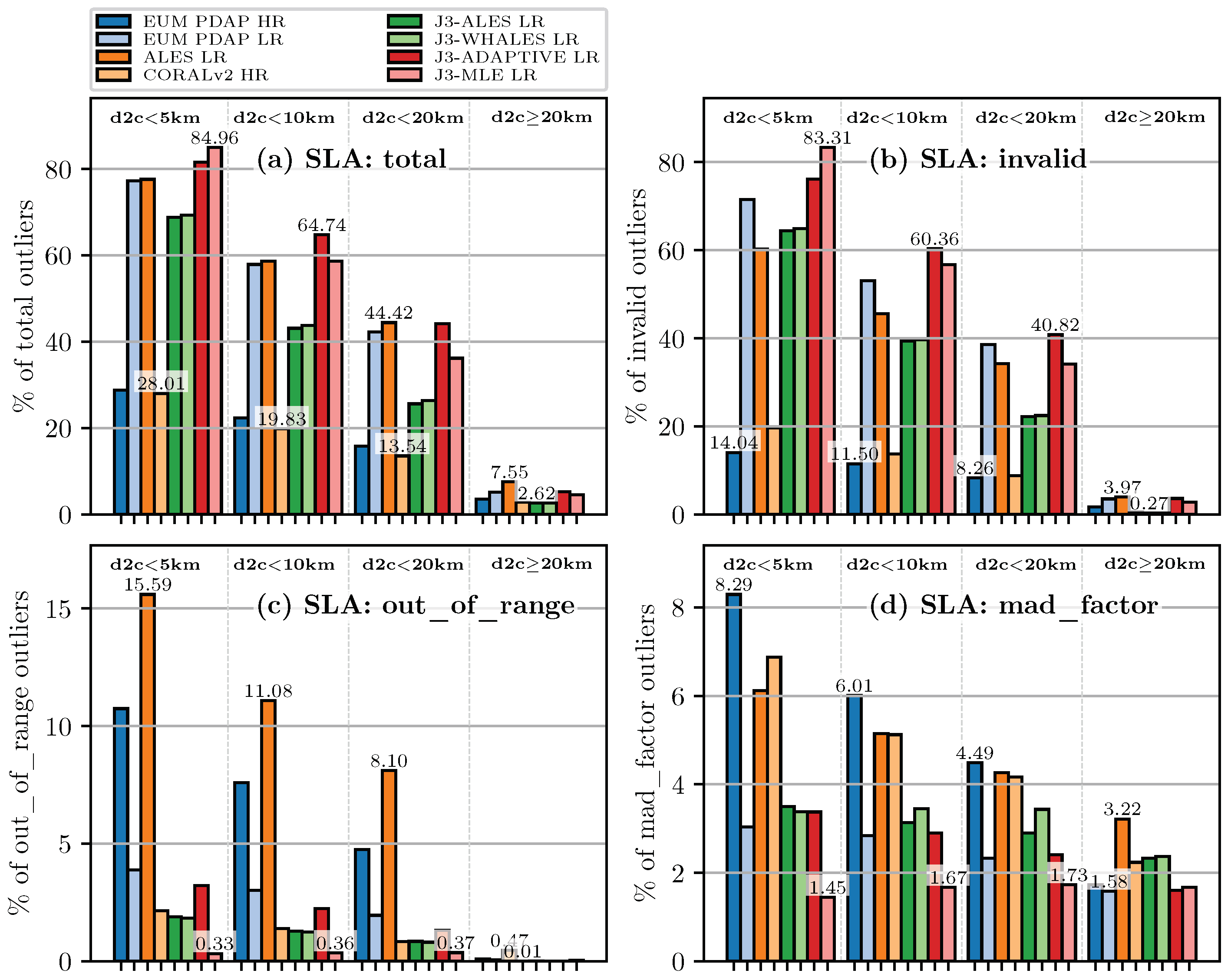
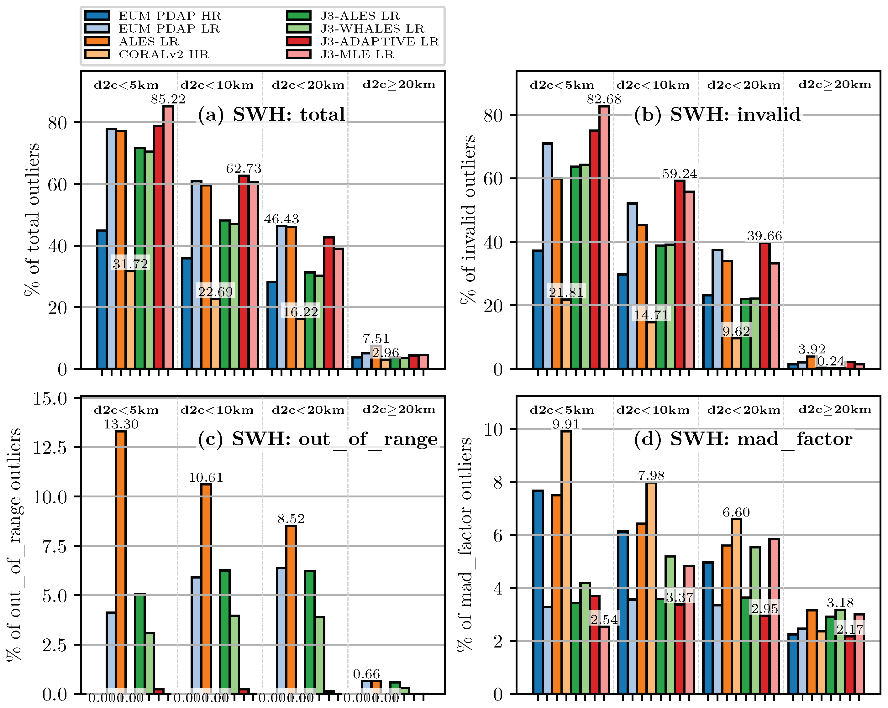
In Figure 1 and Figure 2, the outliers defined in Section 3.1 are evaluated for each dataset of SLA and SWH, respectively. We stress again that we include the missing data in the outliers as well, since they point to the failure of a retracker to extract meaningful physical information from a particular waveform. The following discussion involves the statistics reported for SLA. As it is visible from the figures, we find no differences between the analyses of SLA and SWH. This is expected, since range and SWH are estimated simultaneously in all retrackers considered, and the SLA is then computed using exactly the same geophysical corrections and adjustments for all datasets (except for the SSB, which is specific for each retracker).
The expected increase in the number of outliers is observed when approaching the coast. There are nevertheless notable differences depending on the processing mode and the retracker. The most evident result is that the SAR mode sees a drastic drop in outliers. For SLA, only about 25% of the data are identified as outliers by EUM PDPAP HR and CORAL for distances closer than 5 km to the coast. This is in stark contrast to about 85% of outliers found using the open ocean LR product J3-MLE LR.
Secondly, significant differences are observed among different LR processing results. The standard EUM PDAP LR on S6 is significantly less affected by outliers than J3-MLE LR. This highlights that the standard LR processing is improved in S6 compared to J3 in terms of the validity of the measurements. Still, the fact that fewer outliers are present does not yet imply a better accuracy, which is instead the subject of discussion in the comparison against tide gauges in Section 4.4.
Thirdly, it is observed that the latest J3-ADAPTIVE LR approach does not improve the standard J3-MLE-LR performance in terms of outliers. We report that CNES/CLS was contacted concerning this. They declared this is due to a software coding error impacting J3-ADAPTIVE altimeter data. In fact, for distances closer than 10 and 20 km to the coast, J3-ADAPTIVE LR shows the worst performance with, respectively, over 64% and 44% of outliers. The application of the ALES retracker to J3, on the other hand, reduces the number of J3 outliers by about 10–20% (depending on the distance from the coast).
Finally, it is noted that, in all datasets, the largest amount of outliers concerns invalid retrievals. This speaks to the general reliability of the quality flags associated with each dataset, which identify most of the failed retrievals, as already highlighted by Schlembach et al. [23]. Notable exceptions are EUM PDAP HR and ALES LR for S6, where over 10% of SLA retrievals are classified as out of range in our statistics.
4.2. Along-Track Noise Analysis
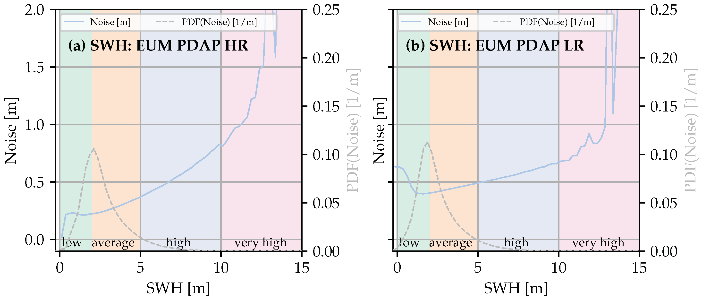
In this section, the along-track noise performance of the datasets in terms of SLA and SWH are analyzed following the methodology described in Section 3.2. Typically, the precision of the parameter estimation in altimetry is a function of the sea state (e.g., [19]). Therefore, it is useful to constrain the validity of our analysis by looking at the distribution of SWH. This is reported in Figure 3 for the open ocean as a probability density function (PDF) together with the noise performance as a function of SWH of the standard S6 datasets EUM PDAP HR and EUM PDAP LR. High and very high sea states are strongly underrepresented and tend to be attenuated in the coastal zone due to sheltering, limited wind fetch, and energy dissipation [10]. As a result, and given the limited dataset that we have processed, the statistics for high and very high sea states are strongly affected by residual outliers in the data: both actually high sea states and erroneously high values are captured in the average.
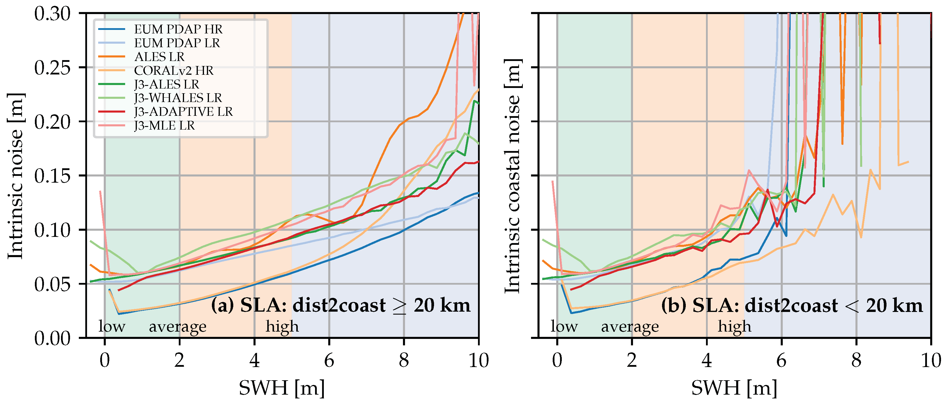
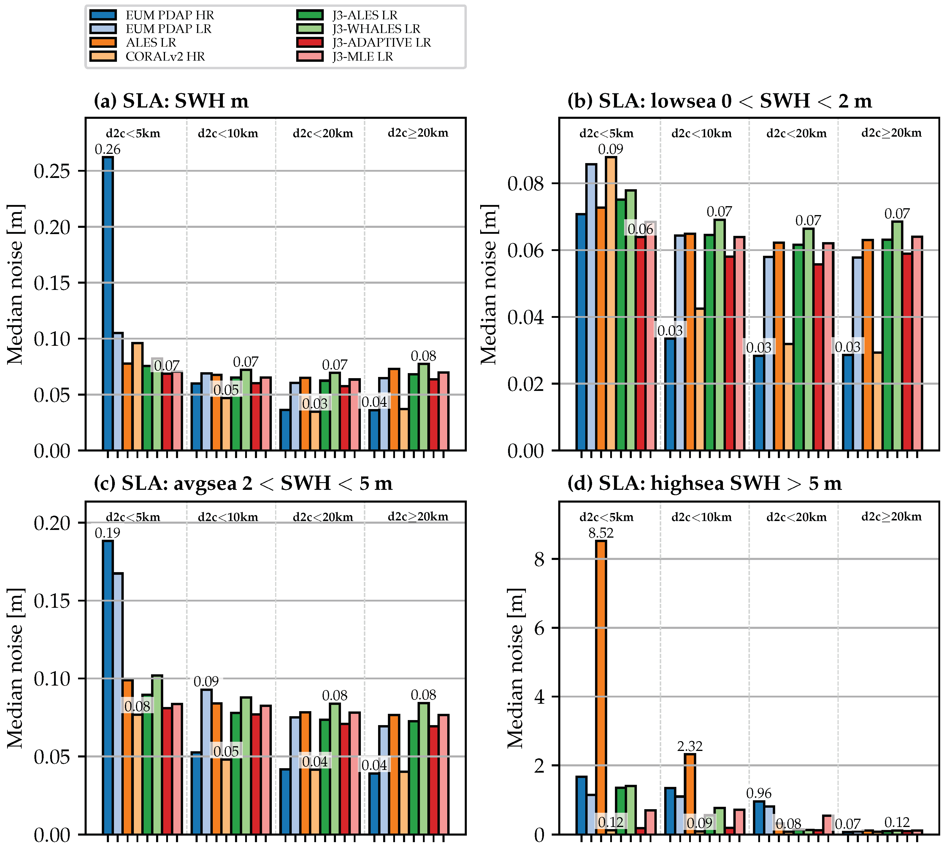
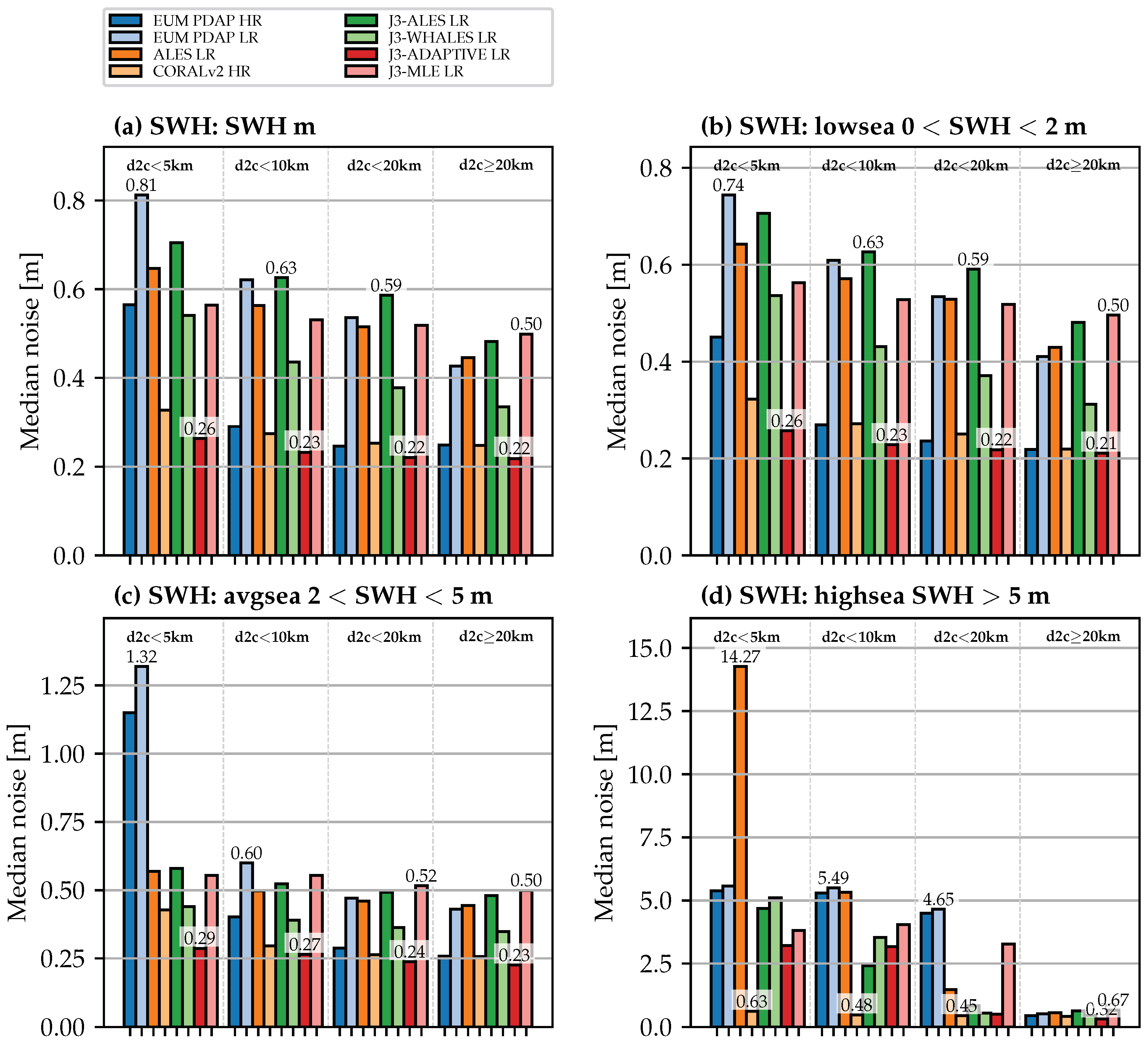
The SLA along-track noise for all datasets is displayed in Figure 4 for distances larger and smaller than 20 km from the coast. The upper limit of the noise is set to 0.3 m here since the higher values for very high sea states are not realistic but instead result from the low number of observations. The statistics are then shown for different sea states and distances to the coast in Figure 5. The same information for SWH along-track noise values are displayed in Figure 6 and Figure 7.
The better precision of both the SAR altimetry dataset EUM PDAP HR and the CORAL dataset stands out. For example, Figure 5 shows that, for average sea states and considering all data within 20 km of the coast, SAR altimetry provides SLA with a precision of about 4 cm, compared to 7.5 cm to 8 cm for the LR datasets. There are nevertheless important differences among the two SAR datasets. In Figure 5a, it can be seen that CORAL is noisier than EUM PDAP HR in the open ocean but succeeds in maintaining realistic noise figures in the coastal zone, where EUM PDAP HR appears to be strongly affected by erroneous estimations. This is particularly relevant considering that, as we have seen in the previous section, CORAL and EUM PDAP HR have similar numbers of valid data. Notably, realistic noise figures are also kept by CORAL in the case of high sea states in the coastal zone, despite the low number of measurements.
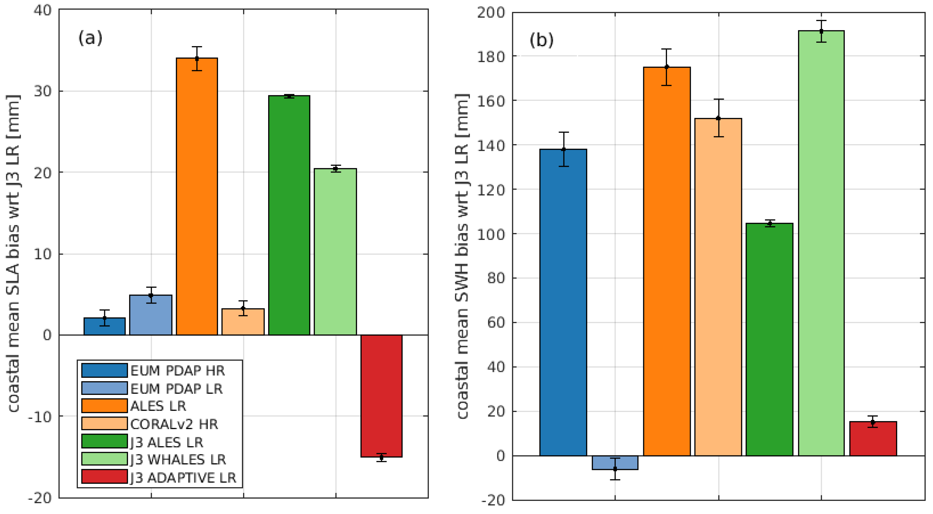
4.3. Bias Analysis
As the data very close to the coast (<10 km) show a large degradation in quality for some of the retrackers, especially for J3-MLE LR, which is used as a reference, the biases are shown for a distance between 10 and 20 km from the coast. Moreover, as it was found that, at least for some retrackers, the mean values depend on the sea state, which in turn correlates with the distance from the coast, only values for SWH between 1 m and 2 m are shown (based on the J3-ADAPTIVE retracker).
4.3.1. Mean Biases in 10–20 km Distance from the Coast
Figure 8 shows the mean biases in the coastal region (10–20 km offshore) for different retrackers. SLA (including SSB correction) is shown in plot (a), and SWH is shown in plot (b).
For SLA, one can see significant biases with respect to J3 LR, which can reach about 3 cm for ALES, and between 1 cm and 2 cm for WHALES and ADAPTIVE. In contrast, both the S6 EUM products (HR and LR) as well as the CORAL retracker only show small biases of less than 5 mm. For SWH, the biases are much larger for most of the retrackers, with up to almost 20 cm for J3 WHALES. Only the S6 HR and the J3-ADAPTIVE show a better agreement with J3 LR. It should be noted, however, that no instrument correction [30] was applied for the ALES/WHALES retracking when computing SWH, resulting in greater inconsistencies with J3 LR and S6 PDAP LR (for which a correction accounting for the Gaussian approximation of the point target response is included) and with J3-ADAPTIVE, (for which such correction is not required, since the real point target response is accounted for in the processing). The high offset for S6 HR depends on the sea state (height and period of waves, as well as sea surface motion) and is also known for the open ocean SWH product, as already documented, for example, in Jiang et al. [31].
The differences in atmospheric corrections between S6 and J3 are small: 2 mm for the smoothed dual-frequency ionospheric correction (“iono_cor_alt_filtered”) and less than 1 mm for the wet troposphere from the radiometer (“rad_wet_tropo_cor”). Neither temporal changes nor correlations to coastal distance can be detected. The corrections for S6 HR and LR are identical.
4.3.2. Dependency on Distance to Coastline
In order to check for possible systematic effects close to the coast, the bias analysis was performed in small distance-to-coast bins, each 10 km wide. Figure 9 shows the S6 SWH biases for different distance-to-coast classes with respect to J3-MLE LR SWH for four different products. The light gray lines indicate the results for the individual cycles, and the bold black line shows the median over all cycles (13–22). These lines are generated on the basis of the full dataset, i.e., all sea states are taken into account. In addition, the orange line shows the median of all cycles using only SWH between 1 m and 2 m. For the full range of SWH, one can clearly see the offset in the HR products and in LR ALES. Moreover, a clear dependence on the distance to the coast can be observed for all datasets. This dependence becomes much smaller when only a specific SWH class is used for the bias calculation. This indicates that there is a dependence on the absolute sea state, as the SWHs are significantly smaller near the coast than in the open ocean [32].
When investigating the bias differences between coastal areas (10–20 km) and the open ocean (20–90 km), no significant offsets (95% confidence level) can be documented, except for the SLA computed with J3-ADAPTIVE (with respect to J3-MLE LR). However, for this retracker too, the bias difference between open and coastal ocean is only 2.8 mm and close to insignificance. These results are based on small waves only (1–2 m). When all sea states are included in the analysis, the differences in SWH between the different retrackers are larger and not always insignificant. This is particularly true for S6 HR (both EUM PDAP and CORAL), indicating a bias in SWH that depends on the sea state itself.
4.3.3. Temporal Bias Evolution
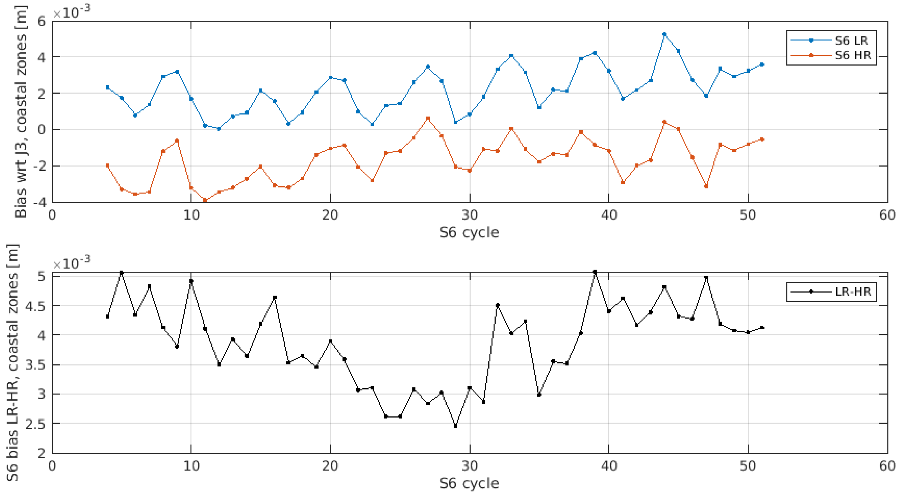
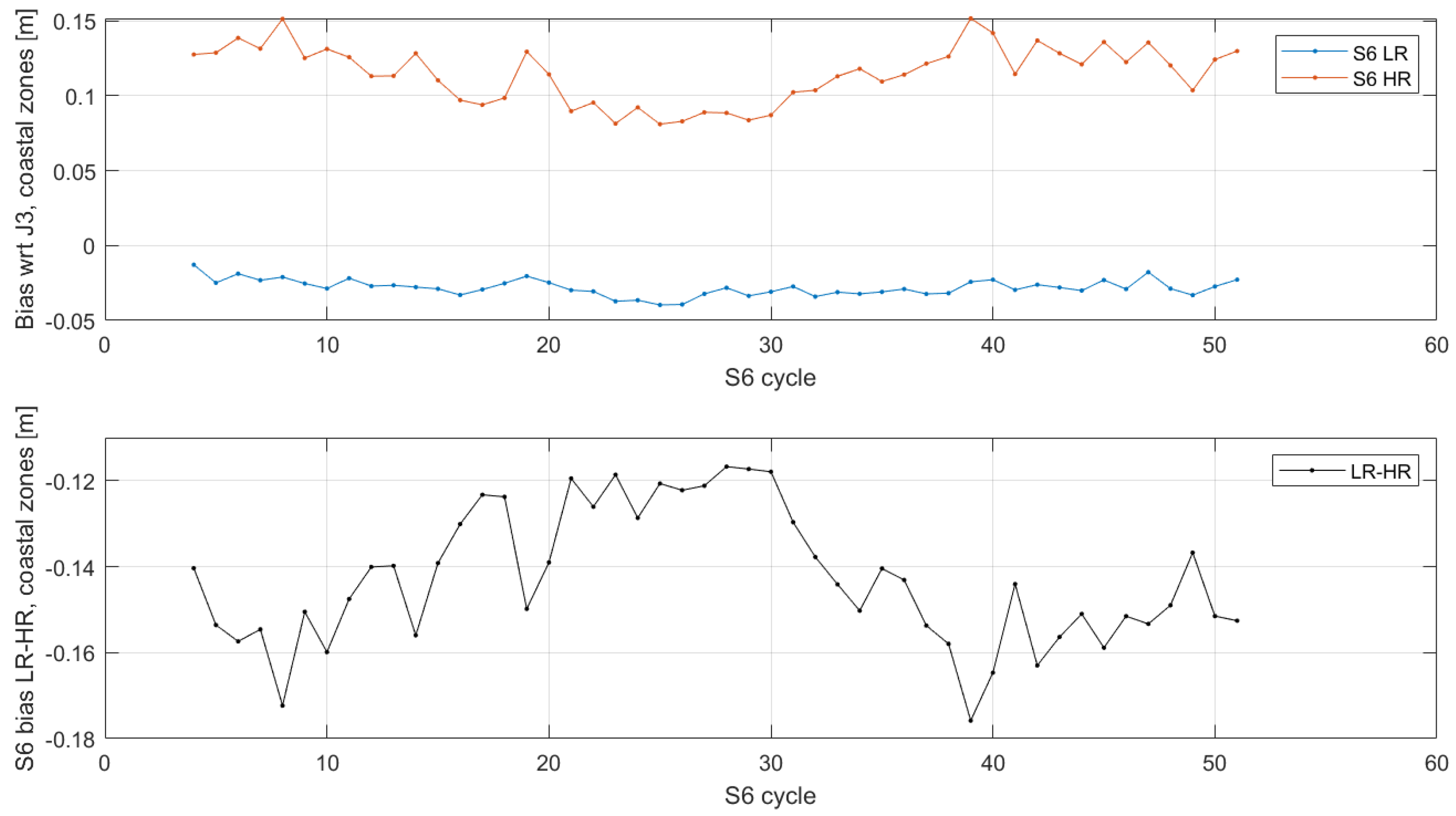
Since the longest possible time series is required for the analysis of temporal bias behavior, only the official level 2 products are considered here. Figure 10 shows the temporal variation of the SLA biases for a bit more than one year (cycles 4–52), while Figure 11 shows the same for the SWH biases. Both are shown on top for S6 in comparison to J3, while the lower plots depict the relationship between S6 LR and HR. The data are based on the full SWH spectrum and cover the coastal areas of 10–20 km. One can identify systematic patterns over time, even if not all of them are mathematically significant. It looks as if, especially in the first half of the time series, both S6 SLA data series show a slight drift which, however, differs between LR and HR. These differences were reported during the S6 commissioning phase to be due to the neglect of the range walk correction in HR processing. In addition, it was shown that the sea-level drift observed between the two missions is caused by the asymmetric evolution of the shape of the point target response, which is not accounted for in the processing [33]. In addition, a jump is observed in the time series of the difference between LR and HR, which occurs at the switch to Poseidon-4 side-B (cycle 31 in September 2021), reinforcing the need to apply numerical retrackers and range-walk correction in the operational data processing chain. For SWH, a kind of annual signal can be seen in S6 HR, but this is not statistically detectable.
4.4. Validation of SLAs against Tide Gauges
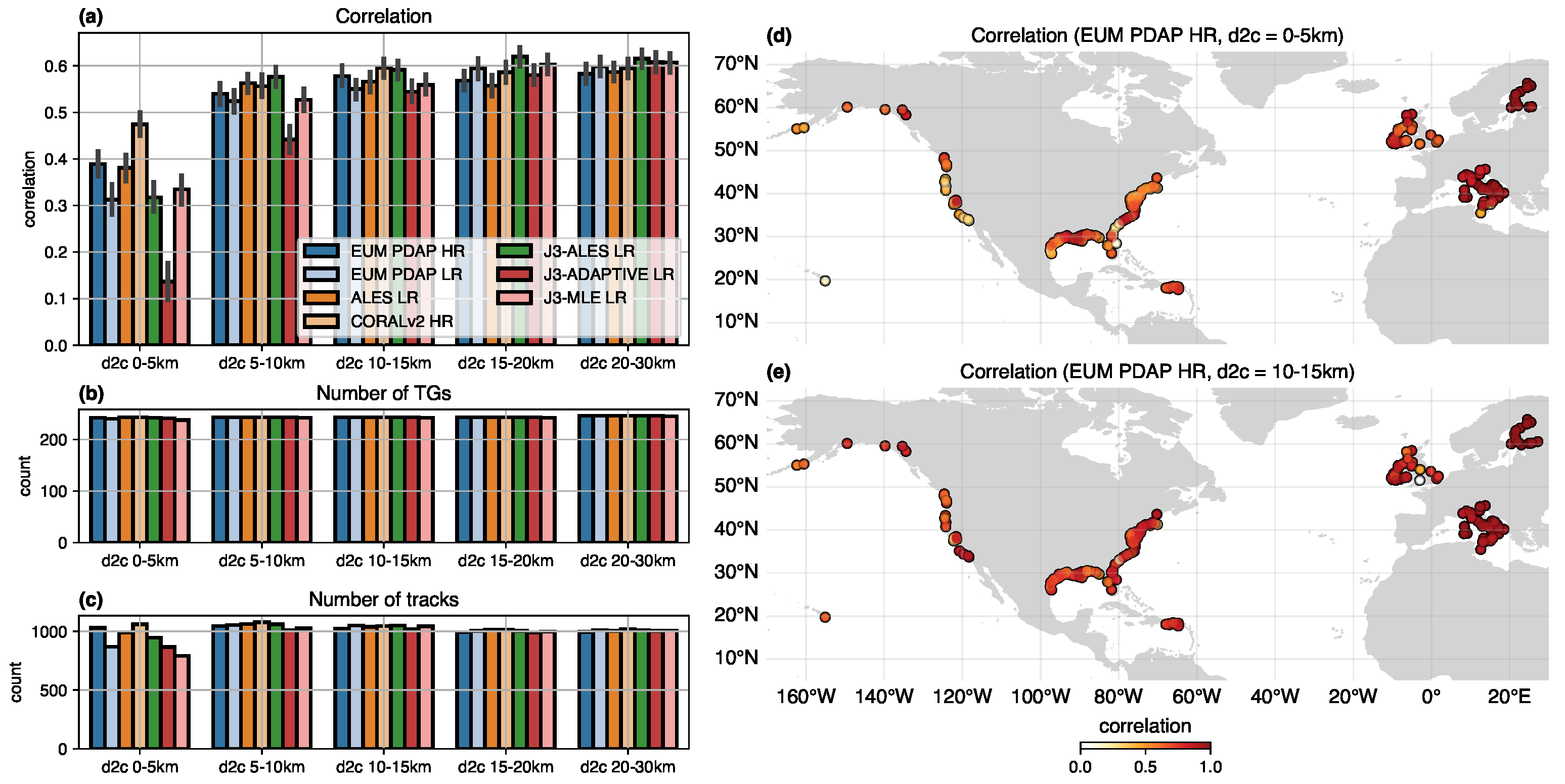
In order to evaluate the coastal accuracy of the products, Figure 12a shows the mean correlation with the tide gauge time series grouped by distance to coast. These numbers are also provided in Table 1. In panels b and c, the number of tide gauges and the number of available tracks for each altimetry dataset are shown. This is an indication of the different amount of valid data for each dataset when approaching the coast, given the different amount of missing or unrealistic sea level estimations, as explained in Section 3.4. Panels d and e show the location of the tide gauges and the correlations with EUM PDAP HR, i.e., the reference product of S6, for two different binned coastal distances.
The first result is that significant differences among the dataset arise in the last 10 km from the coast and are more pronounced in the last 5 km. While coastal dedicated reprocessed altimetry (J3-ALES LR, ALES-LR) is able to reach the same performance as SAR altimetry products within 5 to 10 km, a strong drop in correlation and differences in the quantity of data are seen in the last 5 km. In this region, S6 products significantly outperform J3 products. The best performing dataset is the CORALv2 HR, with an average correlation of 0.47 and the highest amount of used data, demonstrating the added value of dedicated retracking in SAR altimetry. While EUM PDAP HR performs better than its LR counterpart, EUM PDAP LR, the coastal dedicated reprocessing (ALES LR) of S6 LR waveforms increases the performance of the latter in both data quality and quantity. The worst performing dataset in terms of correlation is J3-ADAPTIVE LR in both the 0–5 km and the 5–10 km coastal bin. While J3-ADAPTIVE LR shows great performance in terms of precision of sea state retrievals (see Figure 7), the standard LR processing J3-MLE LR has a better correlation, although fewer data are available.
5. Conclusions
This work has analyzed the coastal performance of J3 and S6 during their tandem phase, with a focus on the coastal zone and on coastal reprocessing algorithms. Our analysis is limited to outlier detection, along-track noise (as a parameter of precision), bias statistics, and correlation with in situ data (as a parameter of accuracy). Two main findings arise from the discussion. Firstly, we can safely say that the official SAR altimetry products are advantageous in the coastal zone with respect to the ones based on the LR mode. For example, the official S6 SLA product from SAR altimetry shows an 8% improvement in our correlation analysis. An exception is the SWH from SAR, which is still biased with respect to the LR record, as already noted in previous studies (e.g., [34]). Secondly, we have demonstrated that dedicated coastal retracking can significantly improve the performance of SAR altimetry as well. Concerning the individual processing methods, we noticed that the ALES retracker for S6 LR (ALES LR) is less precise than its counterpart in J3, meaning that issues in its implementation and differences between the LR mode in the two missions shall be further investigated. Moreover, the ADAPTIVE retracker available in J3 (J3-ADAPTIVE LR), which is known to improve the signal-to-noise ratio of the mesoscales on a global scale [22], is shown to provide an increase in the precision of SWH data but also shows the lowest performance in terms of accuracy against the ground truth for sea level determination in the last 10 km to the coast.
In conclusion, as the final objective of this paper is to provide a coastal assessment of S6 altimetry with respect to J3, our main message is that the official SAR altimetry product EUM PDAP HR achieves coastal performance at the same level as enhanced coastal altimetry reprocessing of LR data (ALES LR, J3-ALES LR) and that its performance can be further improved using a dedicated subwaveform approach applied to the same SAMOSA physical model (CORALv2 HR).
Author Contributions
M.P. coordinated the study, was responsible for the ALES and WHALES retracking, and wrote most of the manuscript. F.S. (Florian Schlembach) organized the datasets and was responsible for the CORAL retracking and the outlier analysis. D.D. performed the bias analysis and wrote the corresponding sections. J.O. was responsible for the tide gauge analysis. F.S. (Florian Seitz) provided the resources making the study possible. All authors have read and agreed to the published version of the manuscript.
Funding
This study was funded by EU and ESA, under ESA Contract No. 4000134346/21/NL/AD.
Data Availability Statement
The data presented in this study are available on request from the corresponding author.
Acknowledgments
The authors are thankful to all the partners of the project “Sentinel-6 Michael Freilich and Jason-3 tandem Flight Exploitation (S6-JTEX)” (ESA Contract No. 4000134346/21/NL/AD), funded by the European Space Agency, for all the fruitful meetings and discussions. In particular, we acknowledge the contribution of Thomas Moreau from CLS.
Conflicts of Interest
The authors declare no conflict of interest.
References
- Chelton, D.B.; Ries, J.C.; Haines, B.J.; Fu, L.L.; Callahan, P.S. Satellite Altimetry. In Satellite Altimetry and Earth Sciences: A Handbook of Techniques and Applications; Fu, L.L., Cazenave, A., Eds.; Academic Press: Cambridge, MA, USA, 2001; Volume 69, pp. 1–131. [Google Scholar] [CrossRef]
- Raney, R.; Phalippou, L. The future of coastal altimetry. In Coastal Altimetry; Vignudelli, S., Kostianoy, A., Cipollini, P., Benveniste, J., Eds.; Springer: Berlin/Heidelberg, Germany, 2011; pp. 535–560. [Google Scholar]
- Garcia, E.S.; Sandwell, D.T.; Smith, W.H. Retracking CryoSat-2, Envisat and Jason-1 radar altimetry waveforms for improved gravity field recovery. Geophys. J. Int. 2014, 196, 1402–1422. [Google Scholar] [CrossRef]
- Wingham, D.; Francis, C.; Baker, S.; Bouzinac, C.; Brockley, D.; Cullen, R.; de Chateau-Thierry, P.; Laxon, S.; Mallow, U.; Mavrocordatos, C.; et al. CryoSat: A mission to determine the fluctuations in Earth’s land and marine ice fields. Adv. Space Res. 2006, 37, 841–871. [Google Scholar] [CrossRef]
- Raney, R.K. Maximizing the intrinsic precision of radar altimetric measurements. IEEE Geosci. Remote Sens. Lett. 2013, 10, 1171–1174. [Google Scholar] [CrossRef]
- Gómez-Enri, J.; Vignudelli, S.; Quartly, G.D.; Gommenginger, C.P.; Cipollini, P.; Challenor, P.G.; Benveniste, J. Modeling ENVISAT RA-2 waveforms in the coastal zone: Case study of calm water contamination. IEEE Trans. Geosci. Remote Sens. 2010, 7, 474–478. [Google Scholar] [CrossRef]
- Fernandes, M.J.; Lázaro, C.; Ablain, M.; Pires, N. Improved wet path delays for all ESA and reference altimetric missions. Remote Sens. Environ. 2015, 169, 50–74. [Google Scholar] [CrossRef]
- Passaro, M.; Cipollini, P.; Vignudelli, S.; Quartly, G.; Snaith, H. ALES: A multi-mission subwaveform retracker for coastal and open ocean altimetry. Remote Sens. Environ. 2014, 145, 173–189. [Google Scholar] [CrossRef]
- Birol, F.; Léger, F.; Passaro, M.; Cazenave, A.; Niño, F.; Calafat, F.M.; Shaw, A.; Legeais, J.F.; Gouzenes, Y.; Schwatke, C.; et al. The X-TRACK/ALES multi-mission processing system: New advances in altimetry towards the coast. Adv. Space Res. 2021, 67, 2398–2415. [Google Scholar] [CrossRef]
- Passaro, M.; Müller, F.; Oelsmann, J.; Rautiainen, L.; Dettmering, D.; Hart-Davis, M.; Abulaitijiang, A.; Andersen, O.; Hoyer, J.; Madsen, K.; et al. Absolute Baltic Sea Level Trends in the Satellite Altimetry Era: A Revisit. Front. Mar. Sci. 2021, 8, 647607. [Google Scholar] [CrossRef]
- Benveniste, J.; Birol, F.; Calafat, F.; Cazenave, A.; Dieng, H.; Gouzenes, Y.; Legeais, J.; Leger, F.; Niño, F.; Passaro, M.; et al. (The Climate Change Initiative Coastal Sea Level Team) Coastal sea level anomalies and associated trends from Jason satellite altimetry over 2002–2018. Sci. Data 2020, 7, 357. [Google Scholar] [CrossRef]
- Mangini, F.; Chafik, L.; Bonaduce, A.; Bertino, L.; Nilsen, J.E.Ø. Sea-level variability and change along the Norwegian coast between 2003 and 2018 from satellite altimetry, tide gauges, and hydrography. Ocean Sci. 2022, 18, 331–359. [Google Scholar] [CrossRef]
- Dinardo, S.; Fenoglio-Marc, L.; Buchhaupt, C.; Becker, M.; Scharroo, R.; Fernandes, M.J.; Benveniste, J. Coastal SAR and PLRM altimetry in german bight and west baltic sea. Adv. Space Res. 2018, 62, 1371–1404. [Google Scholar] [CrossRef]
- Schlembach, F.; Passaro, M.; Dettmering, D.; Bidlot, J.; Seitz, F. Interference-sensitive coastal SAR altimetry retracking strategy for measuring significant wave height. Remote Sens. Environ. 2022, 274, 112968. [Google Scholar] [CrossRef]
- Tran, N.; Labroue, S.; Philipps, S.; Bronner, E.; Picot, N. Overview and update of the sea state bias corrections for the Jason-2, Jason-1 and TOPEX missions. Mar. Geod. 2010, 33, 348–362. [Google Scholar] [CrossRef]
- Taburet, G.; Sanchez-Roman, A.; Ballarotta, M.; Pujol, M.I.; Legeais, J.F.; Fournier, F.; Faugere, Y.; Dibarboure, G. DUACS DT2018: 25 years of reprocessed sea level altimetry products. Ocean Sci. 2019, 15, 1207–1224. [Google Scholar] [CrossRef]
- Andersen, O.; Scharroo, R. Range and Geophysical Corrections in Coastal Regions and Implications for Mean Sea Surface Determination. In Coastal Altimetry; Vignudelli, S., Kostianoy, A., Cipollini, P., Benveniste, J., Eds.; Springer: Berlin/Heidelberg, Germany, 2011; pp. 103–146. [Google Scholar]
- Ray, C.; Martin-Puig, C.; Clarizia, M.P.; Ruffini, G.; Dinardo, S.; Gommenginger, C.; Benveniste, J. SAR Altimeter Backscattered Waveform Model. IEEE Trans. Geosci. Remote Sens. 2015, 53, 911–919. [Google Scholar] [CrossRef]
- Thibaut, P.; Poisson, J.; Bronner, E.; Picot, N. Relative performance of the MLE3 and MLE4 retracking algorithms on Jason-2 altimeter waveforms. Mar. Geod. 2010, 33, 317–335. [Google Scholar] [CrossRef]
- Brown, G.S. The average impulse response of a rough surface and its applications. IEEE Trans. Antennas Propag. 1977, 25, 67–74. [Google Scholar] [CrossRef]
- Hayne, G.S. Radar altimeter mean return waveforms from near-normal-incidence ocean surface scattering. IEEE Trans. Antennas Propag. 1980, 28, 687–692. [Google Scholar] [CrossRef]
- Tourain, C.; Piras, F.; Ollivier, A.; Hauser, D.; Poisson, J.C.; Boy, F.; Thibaut, P.; Hermozo, L.; Tison, C. Benefits of the Adaptive algorithm for retracking altimeter nadir echoes: Results from simulations and CFOSAT/SWIM observations. IEEE Trans. Geosci. Remote Sens. 2021, 59, 9927–9940. [Google Scholar] [CrossRef]
- Schlembach, F.; Passaro, M.; Quartly, G.D.; Kurekin, A.; Nencioli, F.; Dodet, G.; Piollé, J.F.; Ardhuin, F.; Bidlot, J.; Schwatke, C.; et al. Round Robin Assessment of Radar Altimeter Low Resolution Mode and Delay-Doppler Retracking Algorithms for Significant Wave Height. Remote Sens. 2020, 12, 1254. [Google Scholar] [CrossRef]
- Dinardo, S. Techniques and Applications for Satellite SAR Altimetry over Water, Land and Ice; Technische Universität Darmstadt: Darmstadt, Germany, 2020; Volume 56. [Google Scholar] [CrossRef]
- Fenoglio-Marc, L.; Dinardo, S.; Scharroo, R.; Roland, A.; Sikiric, M.D.; Lucas, B.; Becker, M.; Benveniste, J.; Weiss, R. The German Bight: A validation of CryoSat-2 altimeter data in SAR mode. Adv. Space Res. 2015, 55, 2641–2656. [Google Scholar] [CrossRef]
- Haigh, I.D.; Marcos, M.; Talke, S.A.; Woodworth, P.L.; Hunter, J.R.; Haugh, B.S.; Arns, A.; Bradshaw, E.; Thompson, P. GESLA Version 3: A major update to the global higher-frequency sea-level dataset. Geosci. Data J. 2023, 10, 293–314. [Google Scholar] [CrossRef]
- Saraceno, M.; Strub, P.; Kosro, P. Estimates of sea surface height and near-surface alongshore coastal currents from combinations of altimeters and tide gauges. J. Geophys. Res.-Space 2008, 113, C11013. [Google Scholar] [CrossRef]
- Oelsmann, J.; Passaro, M.; Dettmering, D.; Schwatke, C.; Sanchez, L.; Seitz, F. The Zone of Influence: Matching sea level variability from coastal altimetry and tide gauges for vertical land motion estimation. Ocean Sci. 2020, 17, 35–37. [Google Scholar] [CrossRef]
- Carrère, L.; Lyard, F. Modeling the barotropic response of the global ocean to atmospheric wind and pressure forcing-comparisons with observations. Geophys. Res. Lett. 2003, 30, 1275. [Google Scholar] [CrossRef]
- Thibaut, P.; Amarouche, L.; Zanife, O.; Steunou, N.; Vincent, P.; Raizonville, P. Jason-1 altimeter ground processing look-up correction tables. Mar. Geod. 2004, 27, 409–431. [Google Scholar] [CrossRef]
- Jiang, M.; Xu, K.; Wang, J. Evaluation of Sentinel-6 Altimetry Data over Ocean. Remote Sens. 2022, 15, 12. [Google Scholar] [CrossRef]
- Passaro, M.; Hemer, M.; Quartly, G.; Schwatke, C.; Dettmering, D.; Seitz, F. Global coastal attenuation of wind-waves observed with radar altimetry. Nat. Commun. 2021, 12, 3812. [Google Scholar] [CrossRef]
- Dinardo, S.; Cadier, E.; Moreau, T.; Maraldi, C.; Boy, F. Sentinel-6MF Poseidon-4 Main Result from the First Year of Mission from the S6PP LRM and UF-SAR Chain. Ocean Surface Topography Science Team (OSTST) Meeting, Online. 2022. Available online: https://ostst.aviso.altimetry.fr/fileadmin/user_upload/OSTST2022/Presentations/S6VT2022-Sentinel-6-MF_Poseidon-4__Main_results_from_the_first_year_and_half_of_mission_from_the_S6PP_LRM_and_HRM_Chain.pdf (accessed on 21 August 2023).
- Schlembach, F.; Ehlers, F.; Kleinherenbrink, M.; Passaro, M.; Dettmering, D.; Seitz, F.; Slobbe, C. Benefits of fully focused SAR altimetry to coastal wave height estimates: A case study in the North Sea. Remote Sens. Environ. 2023, 289, 113517. [Google Scholar] [CrossRef]
Figure 1.
Comparison of outlier types in the SLA datasets as a function of the distance to the coast.
Figure 1.
Comparison of outlier types in the SLA datasets as a function of the distance to the coast.

Figure 2.
Comparison of outlier types in the SWH datasets as a function of the distance to the coast.
Figure 2.
Comparison of outlier types in the SWH datasets as a function of the distance to the coast.

Figure 3.
Noise level of SWH from the official S6 products and probability density function (PDF) of the records as a function of wave height for HR (a) and LR (b).
Figure 3.
Noise level of SWH from the official S6 products and probability density function (PDF) of the records as a function of wave height for HR (a) and LR (b).

Figure 4.
SLA noise level of the individual retrackers as a function of SWH for open ocean (a) and coastal (b) data with the sea state noted at the bottom.
Figure 4.
SLA noise level of the individual retrackers as a function of SWH for open ocean (a) and coastal (b) data with the sea state noted at the bottom.

Figure 5.
SLA median noise for data grouped by distance to coast. The different panels refer to all sea state conditions (a), low (b), average (c), and high sea state (d). No additional SWH thresholds have been applied.
Figure 5.
SLA median noise for data grouped by distance to coast. The different panels refer to all sea state conditions (a), low (b), average (c), and high sea state (d). No additional SWH thresholds have been applied.

Figure 6.
SWH noise level of the individual retrackers as a function of SWH for open ocean (a) and coastal (b) data, with the sea state noted at the bottom.
Figure 6.
SWH noise level of the individual retrackers as a function of SWH for open ocean (a) and coastal (b) data, with the sea state noted at the bottom.

Figure 7.
SWH median noise for data grouped by distance to coast. The different panels refer to all sea state conditions (a), low (b), average (c), and high sea state (d). No additional SWH thresholds have been applied.
Figure 7.
SWH median noise for data grouped by distance to coast. The different panels refer to all sea state conditions (a), low (b), average (c), and high sea state (d). No additional SWH thresholds have been applied.

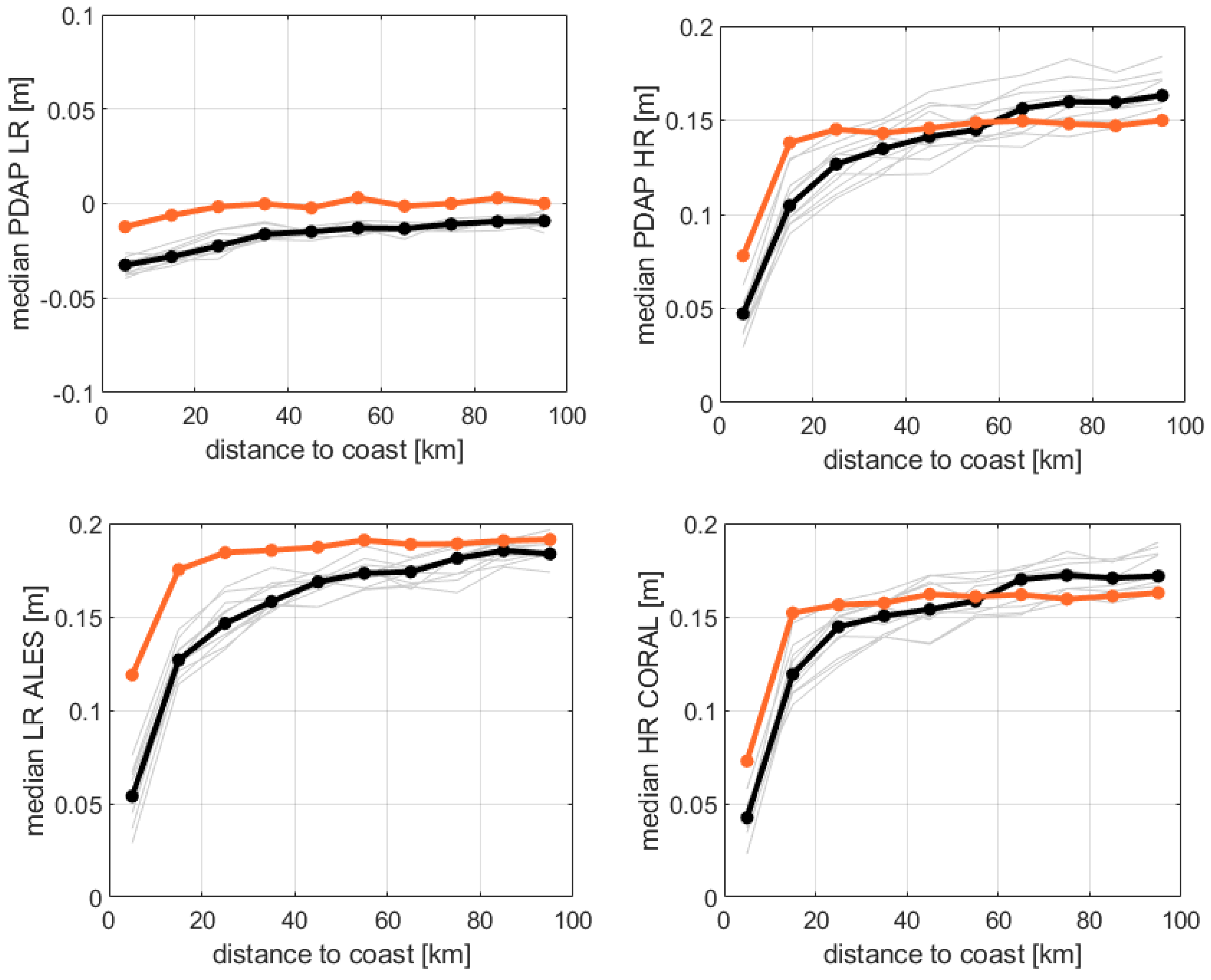
Figure 8.
Mean coastal biases relative to Jason-3 LR for (a) SLA (including SSB) and (b) SWH.

Figure 9.
Coastal dependency of SWH biases for S6 with respect to J3-MLE LR. Top row shows the results for the PDAP products (LR left, HR right); the lower plots are based on two retrackers (ALES LR left, CORAL HR right). Black lines indicate median biases over all cycles for all sea states; orange lines for low sea states only (1–2 m SWH); and gray lines indicate the cycle spread for all sea states.

Figure 10.
Temporal evolution of SLA bias in coastal zones (10–20 km) for all sea states; top: S6 PDAP products with respect to J3-MLE LR; bottom: relative differences between both S6 PDAP products (LR–HR).
Figure 10.
Temporal evolution of SLA bias in coastal zones (10–20 km) for all sea states; top: S6 PDAP products with respect to J3-MLE LR; bottom: relative differences between both S6 PDAP products (LR–HR).

Figure 11.
Temporal evolution of SWH bias in coastal zones (10–20 km) for all sea states; top: S6 PDAP products with respect to J3-MLE LR; bottom: relative differences between both S6 PDAP products (LR–HR).
Figure 11.
Temporal evolution of SWH bias in coastal zones (10–20 km) for all sea states; top: S6 PDAP products with respect to J3-MLE LR; bottom: relative differences between both S6 PDAP products (LR–HR).

Figure 12.
(a) Mean correlations (with 90% confidence intervals) per dataset and distance to coast; (b,c) show number of tide gauges and total number of available tracks for which correlations are computed. These numbers are also an indication of how many data are available in the different datasets; (d,e) show the best correlation per tide gauge for different distances to the coast and for the EUM PDAP HR dataset. One station located west of Hawaii is not shown in (d,e).


Table 1.
Mean correlation between the different altimetry datasets and tide gauges per distance-to-coast class.
Table 1.
Mean correlation between the different altimetry datasets and tide gauges per distance-to-coast class.
| Altimetry Dataset | 0–5 km | 5–10 km | 10–15 km | 15–20 km | 20–30 km |
|---|---|---|---|---|---|
| EUM PDAP HR | 0.39 | 0.54 | 0.58 | 0.57 | 0.58 |
| EUM PDAP LR | 0.31 | 0.52 | 0.55 | 0.59 | 0.60 |
| ALES LR | 0.38 | 0.56 | 0.57 | 0.56 | 0.59 |
| CORALv2 HR | 0.47 | 0.56 | 0.60 | 0.59 | 0.59 |
| J3-ALES LR | 0.32 | 0.58 | 0.59 | 0.62 | 0.62 |
| J3-ADAPTIVE LR | 0.14 | 0.44 | 0.54 | 0.58 | 0.61 |
| J3-MLR LR | 0.33 | 0.53 | 0.56 | 0.60 | 0.61 |
Disclaimer/Publisher’s Note: The statements, opinions and data contained in all publications are solely those of the individual author(s) and contributor(s) and not of MDPI and/or the editor(s). MDPI and/or the editor(s) disclaim responsibility for any injury to people or property resulting from any ideas, methods, instructions or products referred to in the content. |
© 2023 by the authors. Licensee MDPI, Basel, Switzerland. This article is an open access article distributed under the terms and conditions of the Creative Commons Attribution (CC BY) license (https://creativecommons.org/licenses/by/4.0/).
Share and Cite
MDPI and ACS Style
Passaro, M.; Schlembach, F.; Oelsmann, J.; Dettmering, D.; Seitz, F. Coastal Assessment of Sentinel-6 Altimetry Data during the Tandem Phase with Jason-3. Remote Sens. 2023, 15, 4161. https://0-doi-org.brum.beds.ac.uk/10.3390/rs15174161
AMA Style
Passaro M, Schlembach F, Oelsmann J, Dettmering D, Seitz F. Coastal Assessment of Sentinel-6 Altimetry Data during the Tandem Phase with Jason-3. Remote Sensing. 2023; 15(17):4161. https://0-doi-org.brum.beds.ac.uk/10.3390/rs15174161
Chicago/Turabian StylePassaro, Marcello, Florian Schlembach, Julius Oelsmann, Denise Dettmering, and Florian Seitz. 2023. "Coastal Assessment of Sentinel-6 Altimetry Data during the Tandem Phase with Jason-3" Remote Sensing 15, no. 17: 4161. https://0-doi-org.brum.beds.ac.uk/10.3390/rs15174161
Note that from the first issue of 2016, this journal uses article numbers instead of page numbers. See further details here.