Super Resolution of Satellite-Derived Sea Surface Temperature Using a Transformer-Based Model

Abstract

Sea surface temperature (SST) is one of the most important factors related to the ocean and the climate. In studying the domains of eddies, fronts, and current systems, high-resolution SST data are required. However, the passive microwave radiometer achieves a higher spatial coverage but lower resolution, while the thermal infrared radiometer has a lower spatial coverage but higher resolution. In this paper, in order to improve the performance of the super-resolution SST images derived from microwave SST data, we propose a transformer-based SST reconstruction model comprising the transformer block and the residual block, rather than purely convolutional approaches. The outputs of the transformer model are then compared with those of the other three deep learning super-resolution models, and the transformer model obtains lower root-mean-squared error (RMSE), mean bias (Bias), and robust standard deviation (RSD) values than the other three models, as well as higher entropy and definition, making it the better performing model of all those compared.

1. Introduction

Sea surface temperature (SST), an essential variable related to the ocean and the climate, plays a crucial role in the heat, freshwater, and momentum flux exchange at the ocean–atmosphere interface [1]. Changes in sea surface temperature reveal fronts and eddies caused by subsurface heat changes, and eddies are associated with weak SST gradients [2]. Satellite remote sensing is an effective approach to deriving SST with dense spatial resolution on regional and global scales, making eddies, fronts, and current systems visible in SST imagery [3].

Satellite infrared observations of SST have shown capabilities for finer sampling, with a spatial resolution of about 1–4 km; examples include the Visible Infrared Imaging Radiometer Suite (VIIRS) onboard the Suomi National Polar-orbiting Partnership (Suomi NPP) satellite, the advanced geosynchronous radiation imager (AGRI) onboard the Fengyun-4A (FY-4A), and the Moderate Resolution Imaging Spectroradiometer (MODIS) onboard the Terra and Aqua satellites [4]. However, the SST data derived from satellite infrared radiometers are susceptible to interference from weather factors such as clouds, resulting in low spatial coverage. The measurements of SST from passive microwave radiometers are able to penetrate thick cloud layers, enabling all-weather observations, but they have a coarser spatial resolution of about 50–75 km [5]. The identification and tracking of small SST features requires high spatial resolution and frequent revisits [6]. Reconstructing the high-resolution sea surface temperature fields from passive microwave remote sensing SST observations would greatly facilitate our development of a comprehensive understanding of intricate SST features.

Deep learning-based super-resolution image reconstruction is a novel image reconstruction technique that could improve low-resolution images by downscaling with high fidelity [7]. Dong et al. [8] first used the super-resolution convolutional neural network (SRCNN) method with three convolution layers to solve the super-resolution (SR) problem, and achieved great results. In order to enhance the speed and resolution of the model, the fast super-resolution convolutional neural network (FSRCNN) [9] was proposed by Dong et al., which achieved a better super-resolution quality while being tens of times faster than previous models. Kim et al. [10] proposed the very deep SR network (VDSR) method, with 20 layers, to enhance SR performance. They found that deeper work can benefit from the capacity of deep learning-based SR, and the residual learning framework can be useful in solving the gradient explosion problem. A method called the deep compendium model (DCM) was proposed by Haut et al. [11]. It is a novel SR method based on a deep efficient model that integrates improvements on previous network designs, including residual units, skip connections, and network-in-network (NIN), to efficiently acquire high-quality super-resolution remote sensing data while avoiding undesirable visual artifacts.

Deep learning-based super-resolution image reconstruction has been explored in the field of SST and has shown outstanding achievements. In some approaches, the Level 4 SST data are downscaled by interpolating them into low-resolution (LR) SST images, and subsequently upscaling the LR SST images to SR SST images via the deep learning method, which shows that deep learning methods can be used to deal with SST SR problems. For example, Aurelien et al. [12] downscaled the Operational Sea Surface Temperature and Ice Analysis (OSTIA) SST data into LR SST images via bicubic interpolation, and they then chose the SRCNN model to upscale the LR SST images into SR SST images. Khoo et al. [13] proposed the Spectral Normalization–Enhanced Super Resolution Generative Adversarial Network (SN-ESRGAN) to upscale LR SST images into SR SST images. The LR SST images were downscaled from the OSTIA SST data by nearest interpolation. By validating the low-resolution data from the South China Sea, this method can achieve a higher and more realistic resolution than other methods. In other approaches, infrared SST data are selected as high-resolution (HR) data and microwave SST data are selected as LR data to train deep learning methods. Lloyd et al. [14] adopted the VDSR method to upscale the 1 km resolution brightness temperature data from the Sentinel 3 satellite into 200 m resolution SST data, and the target SST data came from the Landsat 8 satellite. Tomoki et al. [15] used the 125 km-resolution ERA20C SST data as the LR SST data and the 25 km resolution OISST SST data as the HR SST data to train the residual in residual dense block (RRDB) net, and the results exhibited a high quality. Bo et al. [5] proposed the oceanic data reconstruction (ODRE) network and trained it with 3-day-averaged 0.25° × 0.25° grid advanced microwave scanning radiometer 2 (AMSR2) SST data and daily 4 km Lever-3 mapped MODIS Terra SST data. The article demonstrates the excellent performance of the ODRE model compared to the FDSR, DRRN, SRCNN, and VDSR models.

The studies mentioned above primarily used CNN as the main network. It is worth noting, however, that the transformer-based model, which incorporates the attention mechanism, has gained significant attention in computer vision applications and has achieved remarkable outcomes. The transformer model has been sought to apply to computer vision tasks, rather than convolutional approaches alone [16,17]. The focus of this paper is on improving the performance of super-resolution SST images derived from microwave SST data. We propose a transformer-based SST reconstruction model, which can upscale the microwave SST data 12.5 times.

The summary is organized as follows: The experimental data are introduced in Section 2.1. The overall framework of the proposed transformer model is presented in Section 2.2.1 and the other three SR models are introduced in Section 2.2.2. Besides, a brief introduction is given to the loss function and implementation details in Section 2.2.3. The results are represented in Section 3 and are discussed in Section 4. The conclusion is given in Section 5.

2. Materials and Methods

2.1. Training Data

The VIIRS_L3S_LEO_PM SST dataset comprises the 0.02° gridded L3S sub-skin SST data produced by the National Oceanic and Atmospheric Administration, Center for Satellite Applications and Research (NOAA STAR) [18]. The data were sourced from the VIIRS onboard the Joint Polar Satellite System (JPSS) satellites; specifically, the Suomi NPP and NOAA20 (N20) satellites. The dataset covers the period from February 2012 to the present, and is reported in two files per 24-hour interval, daytime and nighttime, approximately at the local equator crossing times around 01:30/13:30. The data were provided in NetCDF4 format. The data were downloaded from https://search.earthdata.nasa.gov (accessed on 18 September 2023). The SST image yielded by the VIIRS_L3S_LEO_PM SST dataset on 1 January 2022 is shown in Figure 1.

The AMSR2_L3U SST dataset comprises the 0.25° gridded L3U sub-skin SST data produced by Remote Sensing Systems (REMSS). The data were sourced from the advanced microwave scanning radiometer 2 (AMSR2) sensor onboard the Global Change Observation Mission–Water (GCOM-W) satellite developed by the Japan Aerospace Exploration Agency (JAXA). The dataset covers the period from 2 July 2012 to the present day. The local equator crossing times are at approximately 01:30 and 13:30. The data are provided in NetCDF4 format. The data were downloaded from the website https://data.remss.com/amsr2/ocean/L3/ (accessed on 18 September 2023). The SST image yielded by the AMSR2_L3U SST dataset on 1 January 2022 is shown in Figure 2.

The left and right patches in Figure 3 are truncated from the SST images at the same locations as the AMSR2 and VIIRS, respectively. Figure 1 and Figure 2 clearly show that the passive microwave radiometer represented by the AMSR2 achieves a higher spatial coverage, while the thermal infrared radiometer represented by the VIIRS has a lower spatial coverage. Nevertheless, as shown in Figure 3, the SST image retrieved from the AMSR2 has a lower resolution, while the SST image retrieved from the VIIRS has a higher resolution. Therefore, by adopting the super-resolution method, the resolution of the AMSR2 SST data can be improved, yielding a higher spatial coverage.

Considering the SST for the VIIRS and AMSR2 differ in depth, the value of the VIIRS SST and the AMSR2 SST at daytime is different from that at nighttime because of the strong diurnal warming effect. Therefore, in order to improve the accuracy of results, the nighttime data and daytime data should be taken to train the models, respectively. In this paper, we only discuss the model trained by the nighttime data. There are two years of global nighttime data, 2021 and 2022 SST, used for the training dataset in this study. The global nighttime SST data from January 2023 were used for validation. The AMSR2 and VIIRS data taken on the same day can be interpreted as a low-resolution and high-resolution image pair. The training image pairs were split into 12-by-12 patches in AMSR2 and 150-by-150 patches in VIIRS, and the patches with missing data were excluded. After filtering out missing data, there are 258,738 full patches, which were completely employed as training data in this experiment. Likewise, after filtering out missing data, there are 9469 full patches, which were completely employed as testing data in this experiment. All the training patches and testing images were normalized to the interval [0, 1] before training.

2.2. Methods

Transformer-based models have been widely adopted in the field of computer vision. However, transformer-based deep learning SR models are rarely applied to the SST field at present. Therefore, a transformer-based model is proposed to reconstruct the high-resolution SST fields from passive microwave remote sensing SST observations. In order to verify the accuracy and quality of the outputs of the transformer-based model, three CNN-based SR models are used to compare the statistics of SST difference between the outputs and the VIIRS SST data. The detailed framework of the proposed model is shown as follows.

2.2.1. The Proposed Model

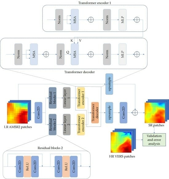
The overall framework of the transformer model is shown in Figure 4. The reason for choosing two groups of ResNet blocks, linear layers, and transformer encoders in parallel is that the DCM has achieved good results using jump connections [11], so we also used jump connections in the design of the proposed model.

Given an LR patch, one convolution is utilized to transform the pixel space input from the AMSR2_L3U SST dataset to feature space.

$${\mathrm{f}}_{\mathrm{i}\mathrm{n}}=\mathrm{c}\mathrm{o}\mathrm{n}\mathrm{v}\left({\mathrm{x}}_{\mathrm{L}\mathrm{R}}\right)$$

(1)

here, $\mathrm{c}\mathrm{o}\mathrm{n}\mathrm{v}$ denotes a convolutional operation and ${\mathrm{x}}_{\mathrm{L}\mathrm{R}}$ represents the LR patch, while ${\mathrm{f}}_{\mathrm{i}\mathrm{n}}$ represents the output tensor of the convolution.

Two residual blocks are borrowed from Res-Net [19] and play a crucial role in image deep learning by aiding in gradient vanishing and exploding. With the introduction of skip connections, these blocks allow for the seamless flow of gradients, mitigating the issues of gradient instability. Furthermore, the residual blocks enhance the fitting capacity of the network by effectively learning residual information, thereby capturing the difference between the input and output features. Therefore, residual blocks not only improve the ability of the model to fit complex patterns, but also accelerate convergence during training. As shown in Figure 5, residual blocks 1 and residual blocks 2 can be constructed by stacking multiple residual blocks, enabling the expression of intricate features and enhancing overall model performance. The convolutions and rectified linear units (ReLUs) are included in the residual blocks, which are defined as

$${\mathrm{x}}_1={\mathrm{R}\mathrm{e}\mathrm{s}}_1\left({\mathrm{f}}_{\mathrm{i}\mathrm{n}}\right)$$

(2)

$${\mathrm{x}}_2={\mathrm{R}\mathrm{e}\mathrm{s}}_2\left({\mathrm{x}}_1\right)$$

(3)

where ${\mathrm{R}\mathrm{e}\mathrm{s}}_1$ and ${\mathrm{R}\mathrm{e}\mathrm{s}}_2$ represent the first and second residual blocks, and ${\mathrm{x}}_1$ and ${\mathrm{x}}_2$ denote the outputs of the first residual block and the second residual block, respectively.

After feature extraction in the feature space, two linear layers can be used to project the input tensor into a higher-dimensional space, thereby enhancing the expressive power of the model. The weights and biases in the linear layer are model parameters that need to be learned through the backpropagation algorithm. By utilizing training data and a loss function, the model can automatically adjust the parameters in the linear layer, enabling the model to fit the training data better and achieve greater generalization. The linear layers are defined as

$${\mathrm{l}}_1={\mathrm{L}\mathrm{i}\mathrm{n}\mathrm{e}\mathrm{a}\mathrm{r}}_1\left({\mathrm{x}}_1\right)$$

(4)

$${\mathrm{l}}_2={\mathrm{L}\mathrm{i}\mathrm{n}\mathrm{e}\mathrm{a}\mathrm{r}}_2\left({\mathrm{x}}_2\right)$$

(5)

where ${\mathrm{L}\mathrm{i}\mathrm{n}\mathrm{e}\mathrm{a}\mathrm{r}}_1$ and ${\mathrm{L}\mathrm{i}\mathrm{n}\mathrm{e}\mathrm{a}\mathrm{r}}_2$ represent the first and second linear layers, and ${\mathrm{l}}_1$ and ${\mathrm{l}}_2$ denote the outputs of the first linear layer and the second linear layer, respectively.

Following the idea of Alexey et al. [16], the standard transformer here receives a one-dimensional sequence of token embeddings as the input. To handle the three-dimensional (3-D) features of patches, we should reshape the patches $\mathrm{l}\in {\mathrm{R}}^{\mathrm{H}\times \mathrm{W}\times \mathrm{C}}$ into sequences of flattened two-dimensional (2-D) vectors ${\mathrm{l}}_{{\mathrm{p}}_{\mathrm{i}}}\in {\mathrm{R}}^{{\mathrm{P}}_{\mathrm{H}}\times {\mathrm{P}}_{\mathrm{W}}\times \mathrm{C}}$, $\mathrm{i}=\{1,\dots ,\mathrm{N}\}$, where $(\mathrm{H},\mathrm{W},\mathrm{C})$ represents the height, the width, and the number of channels of the features, $({\mathrm{P}}_{\mathrm{H}}\times {\mathrm{P}}_{\mathrm{W}}\times \mathrm{C})$ represents the height, the width, and the number of channels of the vectors, and $\mathrm{N}=(\mathrm{H}\mathrm{W}/{\mathrm{P}}_{\mathrm{H}}{\mathrm{P}}_{\mathrm{W}})$ is the number of vectors, and also denotes the length of the input sequence. The input vector size is typically fixed to D dimensions, and we need to use a trainable linear projection to map ${\mathrm{l}}_{{\mathrm{p}}_{\mathrm{i}}}$ to D dimensions. The formula for reshaping the patches is defined as

$${\mathrm{l}}_{\mathrm{k}}=\left[{\mathrm{l}}_{{\mathrm{p}}_0}^{\left(\mathrm{k}\right)},{\mathrm{l}}_{{\mathrm{p}}_1}^{\left(\mathrm{k}\right)},\dots ,{\mathrm{l}}_{{\mathrm{p}}_{\mathrm{N}}}^{\left(\mathrm{k}\right)}\right],\mathrm{k}=1,2$$

(6)

$${\mathrm{y}}_{\mathrm{k}}=\left[{\mathrm{l}}_{{\mathrm{p}}_0}^{\left(\mathrm{k}\right)}\mathrm{S},{\mathrm{l}}_{{\mathrm{p}}_1}^{\left(\mathrm{k}\right)}\mathrm{S},\dots ,{\mathrm{l}}_{{\mathrm{p}}_{\mathrm{N}}}^{\left(\mathrm{k}\right)}\mathrm{S}\right],\mathrm{k}=1,2$$

(7)

where S is the matrix of the linear projection.

Following the original design of Vaswani et al. [20], the multi-headed self-attention (MSA) module enhances the modeling capacity of the transformer encoder by learning different attention focuses from distinct subspaces through the application of the attention mechanism on different linear projection spaces. This enables the model to capture diverse aspects of the input sequence, thereby improving its representational power and generalization performance. The combination process that takes place in the multi-input MSA module can be formulated as

$$\mathrm{A}\mathrm{t}\mathrm{t}\mathrm{e}\mathrm{n}=\mathrm{s}\mathrm{o}\mathrm{f}\mathrm{t}\mathrm{m}\mathrm{a}\mathrm{x}\left(\frac{\mathrm{Q}{\mathrm{K}}^T}{\sqrt{{\mathrm{d}}_{\mathrm{k}}}}\right)$$

(8)

$$\begin{gathered} \mathrm{M}\mathrm{u}\mathrm{l}\mathrm{t}\mathrm{i}\mathrm{H}\mathrm{e}\mathrm{a}\mathrm{d}\left(\mathrm{Q},\mathrm{K},\mathrm{V}\right)=\mathrm{C}\mathrm{o}\mathrm{n}\mathrm{c}\mathrm{a}\mathrm{t}\left({\mathrm{h}\mathrm{e}\mathrm{a}\mathrm{d}}_1,\dots ,{\mathrm{h}\mathrm{e}\mathrm{a}\mathrm{d}}_{\mathrm{h}}\right){\mathrm{W}}^{\mathrm{O}} \\ \mathrm{w}\mathrm{h}\mathrm{e}\mathrm{r}\mathrm{e}{\mathrm{h}\mathrm{e}\mathrm{a}\mathrm{d}}_{\mathrm{i}}=\mathrm{A}\mathrm{t}\mathrm{t}\mathrm{e}\mathrm{n}\left(\mathrm{Q}{\mathrm{W}}_{\mathrm{i}}^{\mathrm{Q}},\mathrm{K}{\mathrm{W}}_{\mathrm{i}}^{\mathrm{K}}\right)\mathrm{V}{\mathrm{W}}_{\mathrm{i}}^{\mathrm{V}} \end{gathered}$$

(9)

where ${\mathrm{d}}_{\mathrm{k}}$ is the dimensions of the features and $\mathrm{h}\mathrm{e}\mathrm{a}\mathrm{d}$ denotes the heads of the MSA module. The ${\mathrm{W}}^{\mathrm{O}}$, ${\mathrm{W}}_{\mathrm{i}}^{\mathrm{Q}}$, ${\mathrm{W}}_{\mathrm{i}}^{\mathrm{K}}$ and ${\mathrm{W}}_{\mathrm{i}}^{\mathrm{V}}$ are parameter matrices and Q, K, and V are the variables decided by the index of related components.

The transformer encoder 1 and decoder are set as examples to provide a clear description about the process of the transformer block, which are carefully shown in Figure 6. And the transformer encoder 2 in the proposed model has the same structure as the encoder 1. The transformer encoder contains a MSA module and a multilayer perceptron (MLP) network. The layer normalization (LN) [21], which helps mitigate the issue of internal covariate shift during the training process and stabilizes the learning procedure of the model, is set before the MSA module and the MLP module. The MLP module has two linear layers as well as a gaussian error linear unit (GELU) [22], which enables the model to learn and represent complex features, thus improving its ability to generalize and make accurate predictions. The overall formula of the encoder can be represented as

$${\mathrm{y}}_{\mathrm{k}}^{\prime }=\mathrm{M}\mathrm{S}\mathrm{A}\left(\mathrm{L}\mathrm{N}\left({\mathrm{y}}_{\mathrm{k}}\right)\right)+{\mathrm{y}}_{\mathrm{k}},\mathrm{k}=1,2$$

(10)

$${\mathrm{z}}_{\mathrm{k}}=\mathrm{M}\mathrm{L}\mathrm{P}\left(\mathrm{L}\mathrm{N}\left({\mathrm{y}}_{\mathrm{k}}^{\prime }\right)\right)+{\mathrm{y}}_{\mathrm{k}}^{\prime },\mathrm{k}=1,2$$

(11)

where ${\mathrm{z}}_{\mathrm{k}}$ is the output of the transformer encoder, with the same dimension as ${\mathrm{y}}_{\mathrm{k}}$.

In addition to the MSA module and MLP network, the transformer decoder also includes a specific MSA module with cross-attention. By calculating attention weights, this module can simultaneously handle the features input by the decoder and connect them with the output derived from encoder 1. This mechanism allows the decoder to fully utilize the contextual information, resulting in the generation of an output sequence corresponding more accurately to the input sequence. It serves as the core component of the decoder. The output of the decoder can be obtained using the following equation

$${\mathrm{z}}_2^{\prime }=\mathrm{M}\mathrm{S}\mathrm{A}\left(\mathrm{L}\mathrm{N}\left({\mathrm{z}}_2\right)\right)+{\mathrm{z}}_2$$

(12)

$${\mathrm{z}}_2^{″}=\mathrm{M}\mathrm{S}\mathrm{A}\left(\mathrm{L}\mathrm{N}\left({\mathrm{z}}_2^{\prime }\right),\mathrm{L}\mathrm{N}\left({\mathrm{z}}_1\right)\right)+{\mathrm{z}}_2^{\prime }$$

(13)

$${\mathrm{z}}_0=\mathrm{M}\mathrm{L}\mathrm{P}\left(\mathrm{L}\mathrm{N}\left({\mathrm{z}}_2^{″}\right)\right)+{\mathrm{z}}_2^{″}$$

(14)

where ${\mathrm{z}}_0$ is the output of the decoder. Then, we reshape the sequences of the flattened 2-D vectors ${\mathrm{z}}_0$ back into patches and use the linear layer to project the higher-dimensional space back to the tensor. After that, we can receive the output ${\mathrm{q}}_0$.

In the up-sample layer, a function of the PyTorch [23] deep learning framework is employed to perform the up-sample operation. Its main purpose is to increase the size of the input tensor to the target size, thereby altering the spatial resolution of the data to meet the requirements. In this paper, the bicubic method is utilized for the up-sampling operation. The up-sample layer can be represented as

$${\mathrm{u}}_0=\mathrm{u}\mathrm{p}\mathrm{s}\mathrm{a}\mathrm{m}\mathrm{p}\mathrm{l}\mathrm{e}\left({\mathrm{q}}_0\right)$$

(15)

$$\mathrm{h}=\mathrm{u}\mathrm{p}\mathrm{s}\mathrm{a}\mathrm{m}\mathrm{p}\mathrm{l}\mathrm{e}\left({\mathrm{x}}_{\mathrm{L}\mathrm{R}}\right)$$

(16)

where ${\mathrm{u}}_0$ is the output of the up-sample layer derived from the front layers, and the $\mathrm{h}$ is directly up-sampled from the low-resolution patches.

Lastly, one convolution is utilized to transform the feature space into the SST pixel space. It can be represented as

$${\mathrm{f}}_{\mathrm{o}\mathrm{u}\mathrm{t}}=\mathrm{c}\mathrm{o}\mathrm{n}\mathrm{v}\left({\mathrm{u}}_0\right)$$

(17)

where ${\mathrm{f}}_{\mathrm{o}\mathrm{u}\mathrm{t}}$ represents the output tensor of convolution.

Finally, after one convolutional layer is applied, the super-resolution HR patch ${\mathrm{x}}_{\mathrm{S}\mathrm{R}}$ is obtained by adding the $\mathrm{r}\mathrm{e}\mathrm{s}\mathrm{i}\mathrm{d}\mathrm{u}\mathrm{a}\mathrm{l}$ and ${\mathrm{f}}_{\mathrm{o}\mathrm{u}\mathrm{t}}$. The final result can be expressed as follows:

$${\mathrm{x}}_{\mathrm{S}\mathrm{R}}=\mathrm{h}+{\mathrm{f}}_{\mathrm{o}\mathrm{u}\mathrm{t}}$$

(18)

2.2.2. Other SR Models

In order to compare the quality of the outputs of the transformer model, three famous deep learning-based SR models, including the FSRCNN, DCM, and VDSR models, are used to generate high-quality super-resolution outputs, which can be compared with the outputs of the transformer model in different comparisons.

As shown in Figure 7, the DCM model [11] consists of two parts, including the feature extractor part and the reconstruction part. In the feature extractor part, there are 12 convolution layers, which can be used to extract the corresponding feature maps. The parametric rectified linear unit (PReLU) functions [24] are set after every convolution layer, which enables us to deal with the decaying ReLU effect and the vanishing gradient problem. In the reconstruction part, an up-sample layer is used to increase the size of the input tensor to the target size. Then, the two branches with the convolution layer and the PReLU function are set to reduce the depth of the input volume. Lastly, the SR patch is the sum of the outputs of the previous layers and of the up-sample layer derived directly from the low-resolution patch.

As shown in Figure 8, the FSRCNN model [9] is typically used in the area of super-resolution imagery. It consists of patch extraction, representation, non-linear mapping, an up-sample layer, and reconstruction. Firstly, a convolution and PReLU function is set in the patch extraction and representation regions. There are five convolution layers and PReLU functions in the non-linear mapping stage. In the up-sample layer, the up-sample function of PyTorch [23] is also used in this model to increase the input size to the target size. At last, a convolution layer without a PReLU function is used for the reconstruction.

As shown in Figure 9, the architecture of the VDSR model primarily comprises patch extraction, non-linear mapping, and reconstruction [10]. Twenty convolution layers are used in this model, except for in the last part, which is followed by batch normalization (BN) and the ReLU. An up-sample layer is set before the last convolution. Similar to the other models, the SR patch is the sum of the outputs of the previous layers and of the up-sample layer taken directly from the low-resolution patch.

2.2.3. Loss Function and Implementation Details

The loss function of all four models is composed of the mean squared error (MSE). Given a low-resolution patch ${\mathrm{x}}_{\mathrm{L}\mathrm{R}}$ and the corresponding high-resolution reference patch ${\mathrm{x}}_{\mathrm{H}\mathrm{R}}$, the loss function can be attained via

$$\mathrm{L}\left(\mathsf{\theta }\right)=\frac{1}{\mathrm{N}}\sum _{\mathrm{i}=1}^{\mathrm{N}}{\left({\mathrm{G}}_{\mathsf{\theta }}\left({\mathrm{x}}_{\mathrm{L}\mathrm{R}}^{\left(\mathrm{i}\right)}\right)-{\mathrm{x}}_{\mathrm{H}\mathrm{R}}^{\left(\mathrm{i}\right)}\right)}^2$$

(19)

where ${\mathrm{G}}_{\mathsf{\theta }}$ refers to the models with parameters $\mathsf{\theta }$, ${\mathrm{G}}_{\mathsf{\theta }}\left({\mathrm{x}}_{\mathrm{L}\mathrm{R}}^{\left(\mathrm{i}\right)}\right)$ is the aforementioned ${\mathrm{x}}_{\mathrm{S}\mathrm{R}}^{\left(\mathrm{i}\right)}$, and $\mathrm{N}$ is the number of training patches.

In the optimization, we used the Adaptive Moment Estimation (Adam) optimizer [25] to train four models, where ${\mathsf{\beta }}_1=0.9$, ${\mathsf{\beta }}_2=0.99$, and $\mathsf{ϵ}={10}^{-8}$. The initial learning rate was set to ${3\times 10}^{-4}$, and the mini-batch size was set to 5. When the loss of a patch is less than ${10}^{-5}$, the training is stopped. These methods were implemented in PyTorch [23], and all experiments were run on an NVIDIA GeForce RTX 3090 graphics card.

3. Results

In this section, numerous measures are used to verify the quality of the transformer model. At first, the scatterplots are presented to show the minimax errors of all four models directly, and the proportion of errors are calculated to clarify the distribution of errors. Then, the statistics of SST difference between the outputs of the VDSR, DCM, FSRCNN and transformer models and the VIIRS SST data are computed to illustrate the accuracy of all four models. At last, the SST images outputted by all four models are displayed to compare the quality of all four models.

To intuitively compare the stability of the results of all four models, we plotted the scatterplots of all the outputs from January 2023 and calculated the proportion of the error distribution. Figure 10 shows that the scatterplots of the output results of the transformer and DCM models are good, and most of the points are concentrated on the 1:1 straight line. However, compared with the outputs of the transformer and DCM models, the outputs of the VDSR and FSRCNN models show certain points with large differences, reaching as high as 5 °C. According to the distributions of the errors, the transformer model yielded a higher percentage of SST difference within the range of 0.1, 0.2, 0.5, and 1 °C compared with the other three models. Conclusively, the transformer model demonstrates distinct characteristics of better overall stability.

To evaluate the accuracy of the super-resolution SST obtained from the four models, the root mean square error (RMSE), mean bias (Bias), and robust standard deviation (RSD) between the outputs and VIIRS SST were calculated. As shown in

Table 1. Statistics of SST difference between the outputs of the VDSR, DCM, FSRCNN, and transformer models and VIIRS SST data. The number in boldface indicates the best performance.

Model	Mean Bias (°C)	RSD (°C)	RMS (°C)	N
Transformer	0.10	0.35	0.48	213,052,500
DCM	0.12	0.37	0.50	213,052,500
FSRCNN	0.13	0.36	0.49	213,052,500
VDSR	0.15	0.35	0.49	213,052,500
Bilinear	0.21	0.43	0.55	213,052,500
Cubic	0.18	0.41	0.53	213,052,500

, the bilinear and cubic interpolation showed a higher bias, RSD, and RMS compared to the deep learning models. Overall, the accuracy of the super-resolution SST values obtained from the deep learning model is slightly higher than that of the bilinear and cubic interpolation. In the comparison of four deep learning models, the transformer model showed the smallest bias and RMS, with values of 0.1 °C and 0.48 °C, respectively. The bias of the VDSR model is relatively high compared to the other three models, with the value of 0.15 °C. Comparing the RSD values of the models helps to exclude some extreme values from interfering with the error analysis, and so it is conducive to deriving a better understanding of the overall error of the data; here, the VDSR model and the transformer model showed the smallest values and thus the better results. Overall, the accuracy of the super-resolution SST values obtained from the transformer model is slightly higher than that of the other three models.

Furthermore, the entropy and definition were employed to assess the quality of the SST images. The definition was measured by the gradient method, and a higher gradient magnitude indicates more pronounced edges or contour changes in the image [26]. Entropy is an important metric for measuring the richness of information [27]. As shown in

Table 2. Entropy and definition of the SST outputs of the VDSR, DCM, FSRCNN, transformer models and AMSR2 SST and VIIRS SST.

	Transformer	DCM	FSRCNN	VDSR	AMSR2	VIIRS	Bilinear	Cubic
Entropy	4.20	4.19	4.19	4.18	4.12	4.24	4.18	4.22
Definition	75.46	57.69	57.40	50.10	3.99	128.08	48.85	52.80

, all models showed similar entropy values, while those of the transformer model and FSRCNN were higher compared to the other two deep learning models. And the entropy of the cubic is the highest. The definition of results of the transformer model are much better than those of the other three models, with a larger value of 75.46. The DCM and FSRCNN showed similar gradients, around 57. Compared with the traditional interpolation method, of bilinear and cubic, the deep learning model performs better in improving the image resolution. Moreover, the definition of the AMSR2 and VIIRS SST images are 3.99 and 128.08. All models can significantly improve the definition of the AMSR2 SST images, but there is still a gap with the definition of those of VIIRS. Overall, the SST image quality was improved through the deep learning models.

In order to demonstrate the spatial pattern of the results, we randomly selected the output from three regions. The super-resolution SST patches from the four models, as well as the AMSR2 SST and VIIRS SST patches, are displayed in Figure 11a. The reconstructions of the transformer and FSRCNN models in the northeastern area of the low-SST region are better than those of the other two models. The SST image generated by the transformer model is better than those of the other three models in the southern low-SST zone. In Figure 11b, the SST image output from the transformer model retains the details of the fronts a little more effectively than the other three models. The fronts of the other three models are either broken or notably weakened, resulting in deviations from actual conditions. In Figure 11c, we can see that the VDSR and DCM models have been over-smoothed, resulting in losses of detail. The SST images outputted by the transformer and FSRCNN models reflect the low-temperature region in the middle of the image, indicating that the quality of their reconstruction is high in this patch.

4. Discussion

The transformer model achieves the lower bias, RSD, and RMS values, while obtaining higher values of entropy and definition, suggesting that the transformer block and the residual block benefit in SST reconstruction. Additionally, it effectively generates the distributions of absent temperature values in low-resolution data. These findings suggest that the transformer block and residual block included in the transformer-based model are useful for reducing pixel-by-pixel inaccuracies in the super-resolution sea surface temperature data. The accuracy of the DCM model is lower than that of the transformer model and higher than that of the VDSR model. This is because the DCM model features skip connections and NIN, allowing the model to acquire a better understanding of the relation between low-resolution SST data and high-resolution SST data. As a result, the DCM model is capable of generating more accurate outputs than the FSRCNN and VDSR models.

To further investigate the accuracy of the transformer model, we have drawn patches from the outputs of the transformer model, the AMSR2 SST, and the VIIRS SST, and we have also plotted the corresponding SST histograms of the outputs of the transformer models, and of the VIIRS SST and SSIM images. The patches of three days are arbitrarily chosen as examples. The patches of 10 January 2023 are shown in Figure 12a–e. The comparison of the AMSR2 SST, VIIRS SST, and SR SST images shows that the transformer model removes the artificial low-temperature region in the southeastern part of the AMSR2 SST image, and at the same time enhances the real high-temperature region in the southwest part of the SST image, making the result more consistent with that of the VIIRS. The histogram of the output SST also shows that its distribution is basically consistent with the distribution shown in the VIIRS SST. At the same time, the SSIM images also show a high degree of similarity, with the SSIM values of most regions being above 0.98, and only a small number of regions having lower SSIM values; however, these latter are still above 0.9, which reflects the excellent performance of the transformer model. The patches of 20 January 2023 are shown in Figure 12f–l. The reconstruction of the low-temperature region in the northeastern area of the output of the transformer model is perfect, and the low-temperature region in the middle of the image also matches closely to the trend of VIIRS, which indicates the good performance of the transformer model. Meanwhile, we can see that the distribution of the output SST is similar to that of the VIIRS SST, and we can also see from the SSIM image that the overall SSIM value is still above 0.95, indicating similar results to those of VIIRS. The patches of 9 January 2023 are shown in Figure 12m–o. We can see that the transformer model is corrected in the high-temperature area in the southeastern region compared with the AMSR2 SST, yielding a result that is close to that of the VIIRS SST image. Meanwhile, in the low-temperature region that can be seen in the northwestern region, the trend of the output SST is closer to that of the VIIRS SST, which indicates that the reconstruction is more effective. Additionally, in the SST distribution histogram, there are slight differences amongst the highest values, but on the whole, the SST distribution of the output results is consistent with that of the VIIRS SST. In the SSIM image, all the distributions are basically above 0.94, which indicates the high quality of the output images. The output of the transformer model gained fine features in comparison to that of the AMSR2 SST image, while it remains close to the VIIRS SST image. The histogram of the distribution of SST closely matches the VIIRS SST histogram, and the difference in the SSIM value between the VIIRS SST and the output SST is large, indicating that the transformer model achieves better results in SST super-resolution.

As revealed by Figure 12, the output of the transformer model yields a similar temperature distribution to that seen in the high-resolution SST data and yields a higher accuracy and perceptual quality. In order to assess the contribution of the individual structures of the model, we designed three ablation experiments. Whether two groups of ResNet blocks, linear layers, and transformer encoders or not are included in the transformer model in parallel is the first thing we think about. The result of this experiment indicates that the accuracy of the super-resolution SST values obtained from the transformer model with two groups is higher than that obtained from the transformer model with one group in ablation studies. Therefore, it makes sense that there are two groups of ResNet blocks, linear layers, and transformer encoders in parallel in the structure of the transformer. Secondly, we designed an ablation study regarding the transformer blocks, the result of which showed that when comparing results before removing the transformer blocks, the model without transformer blocks achieves higher bias, RSD, and RMS values, while obtaining lower values of entropy and definition, suggesting that the transformer block learns various attentional focuses from different subspaces, enhancing the modeling capability of the transformer encoder. Lastly, we added an ablation study regarding the residual blocks. The result of the experiment is that when comparing results before removing the residual blocks, the model without residual blocks achieves higher bias, RSD, and RMS values, while obtaining lower values of entropy and definition, suggesting that the residual blocks address the issue of vanishing and exploding gradients by implementing jump connections, which facilitate a smooth gradient flow. Residual blocks are also capable of efficiently learning residual information and capturing distinctions between input and output properties, resulting in an improved network fitting capability and faster convergence rates during training. Incorporating multiple residual blocks to the learn complex features of SST data enhances the overall performance of the model. Nevertheless, in certain regions, a contrast arises between the output of the proposed model and the high-resolution SST data. This discrepancy is primarily found in the near-shore area, and is caused by the error of microwave SST data. As the models used in this study were trained using global SST data, it is possible that a single model may not provide better results for every sea. Furthermore, as in prior research, we can infer that models designed for a specific region tend to perform better than globally trained models, which underscores the importance of regional specialization.

5. Conclusions

It is widely acknowledged that high-resolution SST has a crucial role in the research of the domains of eddies, fronts, and current systems. The SST data from satellite infrared radiometers has a finer sampling but acquires a lower spatial coverage, resulting from the clouds. Nevertheless, satellite measurements of SST from passive microwave radiometers have demonstrated the capability of allowing all-weather observations but have a coarser spatial resolution. Therefore, in order to understand the intricate SST features, the transformer-based SR model proposed in this paper offers a flexible and efficient way to extract the high-resolution sea surface temperature fields from passive microwave remote sensing SST observations. The proposed model comprises the transformer block and the residual block, rather than purely convolutional approaches. The transformer block learns various attentional focuses from different subspaces, enhancing the modeling capability of the transformer encoder. And the residual blocks are capable of efficiently learning residual information and capturing distinctions between input and output properties, resulting in an improved network fitting capability and faster convergence rates during training. Because of the transformer block and the residual block, this transformer-based model obtains lower RMSE, Bias, and RSD values than the other three models, as well as a higher entropy and definition, making it the better-performing model of all compared. The results of this study demonstrate that this transformer-based model represents a viable means to produce SR SST data from LR microwave SST data, the outcomes of which align relatively with the SST values derived from the target dataset, indicating that advanced deep learning methods are suitable not only for the image field, but also for the SST field.

References

- Yang, C.; Leonelli, F.E.; Marullo, S.; Artale, V.; Beggs, H.; Nardelli, B.B.; Chin, T.M.; De Toma, V.; Good, S.; Huang, B.; et al. Sea Surface Temperature Intercomparison in the Framework of the Copernicus Climate Change Service (C3S). J. Clim. 2021, 34, 5257–5283. [Google Scholar] [CrossRef]
- Tandeo, P.; Chapron, B.; Ba, S.; Autret, E.; Fablet, R. Segmentation of Mesoscale Ocean Surface Dynamics Using Satellite SST and SSH Observations. IEEE Trans. Geosci. Remote Sens. 2014, 52, 4227–4235. [Google Scholar] [CrossRef]
- Carroll, A.G.; Armstrong, E.M.; Beggs, H.M.; Bouali, M.; Casey, K.S.; Corlett, G.K.; Dash, P.; Donlon, C.J.; Gentemann, C.L.; Høyer, J.L.; et al. Observational Needs of Sea Surface Temperature. Front. Mar. Sci. 2019, 6, 420. [Google Scholar] [CrossRef]
- Chin, T.M.; Vazquez-Cuervo, J.; Armstrong, E.M. A multi-scale high-resolution analysis of global sea surface temperature. Remote Sens. Env. 2017, 200, 154–169. [Google Scholar] [CrossRef]
- Ping, B.; Su, F.; Han, X.; Meng, Y. Applications of Deep Learning-Based Super-Resolution for Sea Surface Temperature Reconstruction. IEEE J. Stars 2021, 14, 887–896. [Google Scholar] [CrossRef]
- Martin, S. An Introduction to Ocean Remote Sensing; Cambridge University Press: Cambridge, UK, 2014; pp. 86–89. ISBN 978-1-107-01938-6. [Google Scholar]
- Sato, H.; Fujimoto, S.; Tomizawa, N.; Inage, H.; Yokota, T.; Kudo, H.; Fan, R.; Kawamoto, K.; Honda, Y.; Kobayashi, T.; et al. Impact of a Deep Learning-based Super-resolution Image Reconstruction Technique on High-contrast Computed Tomography: A Phantom Study. Acad. Radiol. 2023, 30, 2657–2665. [Google Scholar] [CrossRef] [PubMed]
- Dong, C.; Loy, C.C.; He, K.; Tang, X. Image Super-Resolution Using Deep Convolutional Networks. IEEE Trans. Pattern Anal. Mach. Intell. 2016, 38, 295–307. [Google Scholar] [CrossRef] [PubMed]
- Dong, C.; Loy, C.C.; Tang, X. Accelerating the Super-Resolution Convolutional Neural Network. In Proceedings of the Computer Vision–ECCV 2016: 14th European Conference, Amsterdam, The Netherlands, 11–14 October 2016; Leibe, B., Matas, J., Sebe, N., Welling, M., Eds.; Springer International Publishing: Cham, Switzerland, 2016; pp. 391–407. [Google Scholar] [CrossRef]
- Kim, J.; Lee, J.K.; Lee, K.M. Accurate Image Super-Resolution Using Very Deep Convolutional Networks. In Proceedings of the 2016 IEEE Conference on Computer Vision and Pattern Recognition (CVPR), Las Vegas, NV, USA, 27–30 June 2016; pp. 1646–1654. [Google Scholar]
- Haut, J.M.; Paoletti, M.E.; Fernandez-Beltran, R.; Plaza, J.; Plaza, A.; Li, J. Remote Sensing Single-Image Superreso-lution Based on a Deep Compendium Model. IEEE Geosci. Remote Sens. Lett. 2019, 16, 1432–1436. [Google Scholar] [CrossRef]
- Ducournau, A.; Fablet, R. Deep Learning for Ocean Remote Sensing: An Application of Convolutional Neural Networks for Super-Resolution on Satellite-Derived SST Data. In Proceedings of the 2016 9th Iapr Workshop On Pattern Recognition in Remote Sensing (Prrs), Cancun, Mexico, 4 December 2016. [Google Scholar] [CrossRef]
- Khoo, J.J.D.; Lim, K.H.; Pang, P.K. Deep Learning Super Resolution of Sea Surface Temperature on South China Sea. In Proceedings of the 2022 International Conference on Green Energy, Computing and Sustainable Technology (GECOST), Miri Sarawak, Malaysia, 26–28 October 2022; pp. 176–180. [Google Scholar] [CrossRef]
- Lloyd, D.T.; Abela, A.; Farrugia, R.A.; Galea, A.; Valentino, G. Optically Enhanced Super-Resolution of Sea Surface Temperature Using Deep Learning. IEEE Trans. Geosci. Remote Sens. 2022, 60, 1–14. [Google Scholar] [CrossRef]
- Izumi, T.; Amagasaki, M.; Ishida, K.; Kiyama, M. Super-resolution of sea surface temperature with convolutional neural network and generative adversarial network-based methods. J. Water Clim. Chang. 2022, 13, 1673–1683. [Google Scholar] [CrossRef]
- Dosovitskiy, A.; Beyer, L.; Kolesnikov, A.; Weissenborn, D.; Zhai, X.; Unterthiner, T.; Dehghani, M.; Minderer, M.; Heigold, G.; Gelly, S.; et al. An Image is Worth 16 × 16 Words: Transformers for Image Recognition at Scale. arXiv 2020, arXiv:2010.11929. [Google Scholar] [CrossRef]
- Lei, S.; Shi, Z.; Mo, W. Transformer-Based Multistage Enhancement for Remote Sensing Image Super-Resolution. IEEE Trans. Geosci. Remote Sens. 2022, 60, 1–11. [Google Scholar] [CrossRef]
- Jonasson, O.; Gladkova, I.; Ignatov, A.; Kihai, Y. Algorithmic Improvements and Consistency Checks of the NOAA Global Gridded Super-Collated SSTs from Low Earth Orbiting Satellites (L3S-LEO). In Proceedings of the Ocean Sensing and Monitoring XIII, Online. 12–16 April 2021; Volume 11752. [Google Scholar] [CrossRef]
- He, K.; Zhang, X.; Ren, S.; Sun, J. Deep Residual Learning for Image Recognition. In Proceedings of the 2016 IEEE Conference on Computer Vision and Pattern Recognition (CVPR), Las Vegas, NV, USA, 27–30 June 2016; pp. 770–778. [Google Scholar] [CrossRef]
- Vaswani, A.; Shazeer, N.; Parmar, N.; Uszkoreit, J.; Jones, L.; Gomez, A.N.; Kaiser, A.; Polosukhin, I. Attention is all you need. arXiv 2017, arXiv:1706.03762. [Google Scholar] [CrossRef]
- Ba, J.L.; Kiros, J.R.; Hinton, G.E. Layer normalization. arXiv 2016, arXiv:1607.06450. [Google Scholar] [CrossRef]
- Hendrycks, D.; Gimpel, K. Gaussian error linear units (gelus). arXiv 2016, arXiv:1606.08415. [Google Scholar] [CrossRef]
- Paszke, A.; Gross, S.; Massa, F.; Lerer, A.; Bradbury, J.; Chanan, G.; Killeen, T.; Lin, Z.; Gimelshein, N.; Antiga, L.; et al. PyTorch: An Imperative Style, High-Performance Deep Learning Library. arXiv 2019, arXiv:1912.01703. [Google Scholar] [CrossRef]
- Xu, B.; Wang, N.; Chen, T.; Li, M. Empirical evaluation of rectified activations in convolutional network. arXiv 2015, arXiv:1505.00853. [Google Scholar] [CrossRef]
- Kingma, D.P.; Ba, J. Adam. A method for stochastic optimization. arXiv 2014, arXiv:1412.6980. [Google Scholar] [CrossRef]
- Huang, J.; Mumford, D. Statistics of natural images and models. In Proceedings of the 1999 IEEE Computer Society Conference on Computer Vision and Pattern Recognition (Cat. No PR00149), Fort Collins, CO, USA, 23–25 June 1999; pp. 541–547. [Google Scholar] [CrossRef]
- Jost, L. Entropy and diversity. Oikos 2006, 113, 363–365. [Google Scholar] [CrossRef]
Figure 1.
The SST image of VIIRS on 1 January 2022.
Figure 2.
The SST image of AMSR2 on 1 January 2022.
Figure 3.
The patches of (a) VIIRS and (b) AMSR2 on 1 January 2022.
Figure 4.
Flowchart of the proposed model.
Figure 5.
Illustration of the residual blocks.
Figure 6.
Illustration of the transformer encoder 1 and decoder.
Figure 7.
Flowchart of the DCM model.
Figure 8.
Flowchart of the FSRCNN model.
Figure 9.
Flowchart of the VDSR model.
Figure 10.
Density scatterplots of the VIIRS SST and the super-resolution SST values yielded using the (a) transformer, (b) DCM, (c) FSCNN, and (d) VDSR models, where the line is the 1:1 line. The number is shown in logarithmic form.
Figure 11.
Exemplary SST patches for AMSR2 SST, VIIRS SST, and the super-resolution SSTs of FSRCNN, transformer, VDSR, and DCM on (a) 12 January 2023, (b) 7 January 2023, and (c) 28 January 2023.
Figure 12.
Exemplary SST patches for AMSR2 SST, VIIRS SST, and the super-resolution SSTs of transformer model, histograms of SST between super-resolution SST and VIIRS SST, and SSIM between super-resolution SST and VIIRS SST on (a–e) 10 January 2023, (f–j) 20 January 2023, (k–o) 9 January 2023. In the histograms, the pink bars represent the frequency of VIIRS SST values, while the green bars represent the frequency of SR SST values. In the SSIM image, the lighter the color, the greater the similarity.