

Insights for Estimating and Predicting Reservoir Sedimentation Using the RUSLE-SDR Approach: A Case of Darbandikhan Lake Basin, Iraq–Iran

 ,
,  , and
, and 
Abstract
:1. Introduction
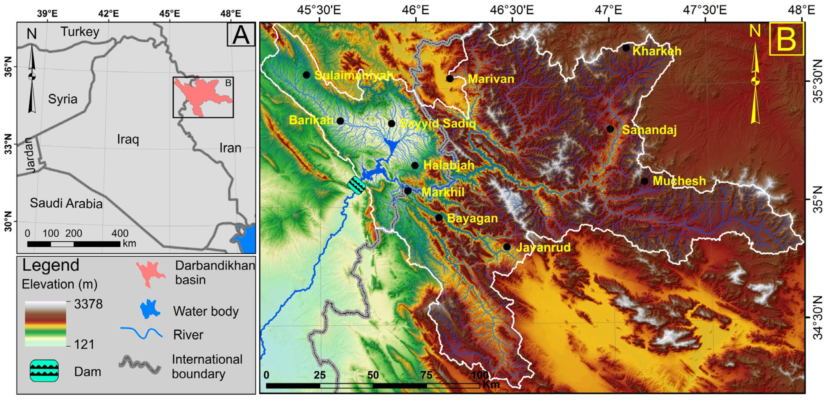
2. Darbandikhan Basin
3. Materials and Methods
3.1. Materials
3.2. Methods
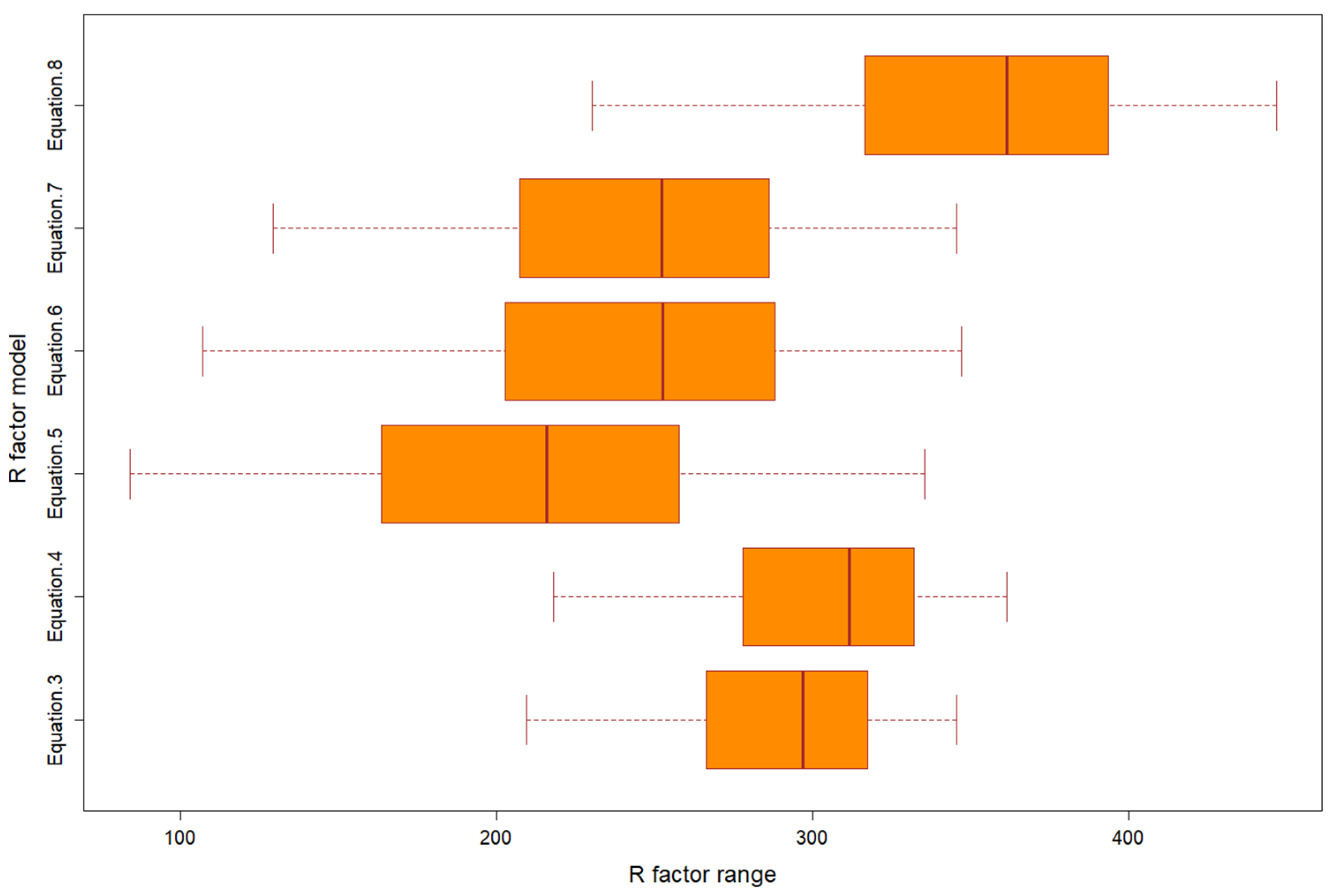
3.2.1. Rainfall and Runoff Erosivity (R Factor)
3.2.2. Soil Erodibility (K Factor)
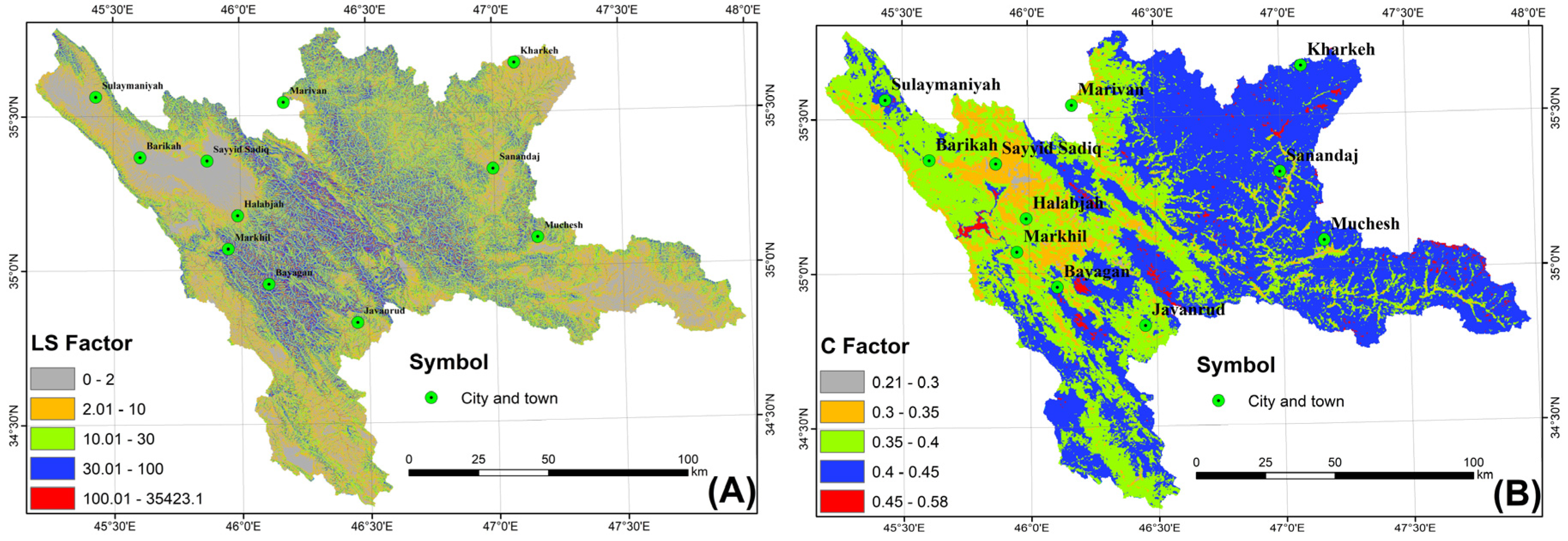
3.2.3. Slope Length (L Factor) and Slope Steepness (S Factor)
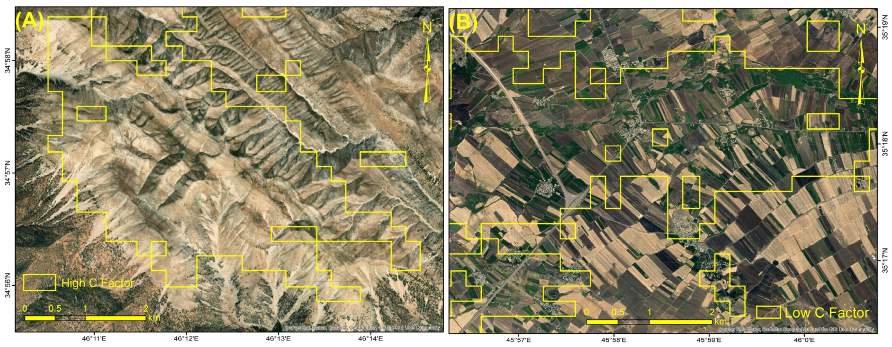
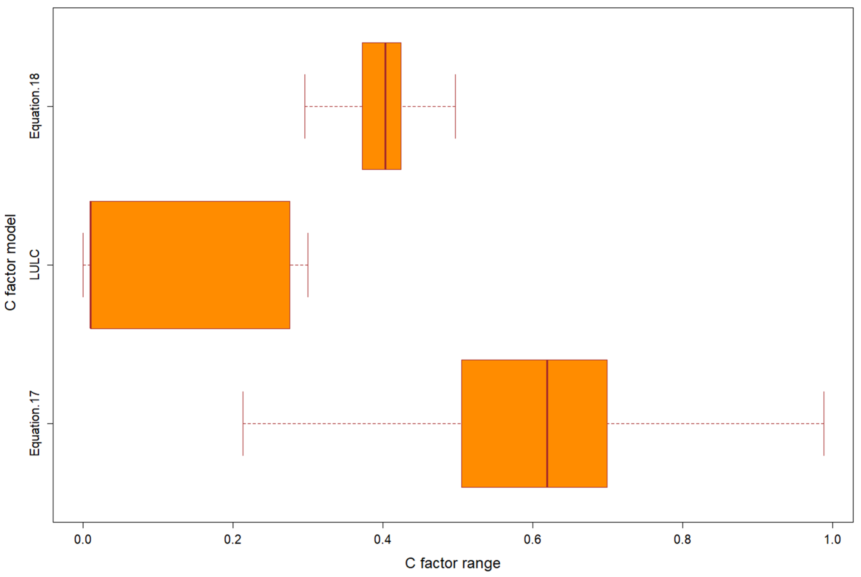
3.2.4. Cover and Management (C Factor)
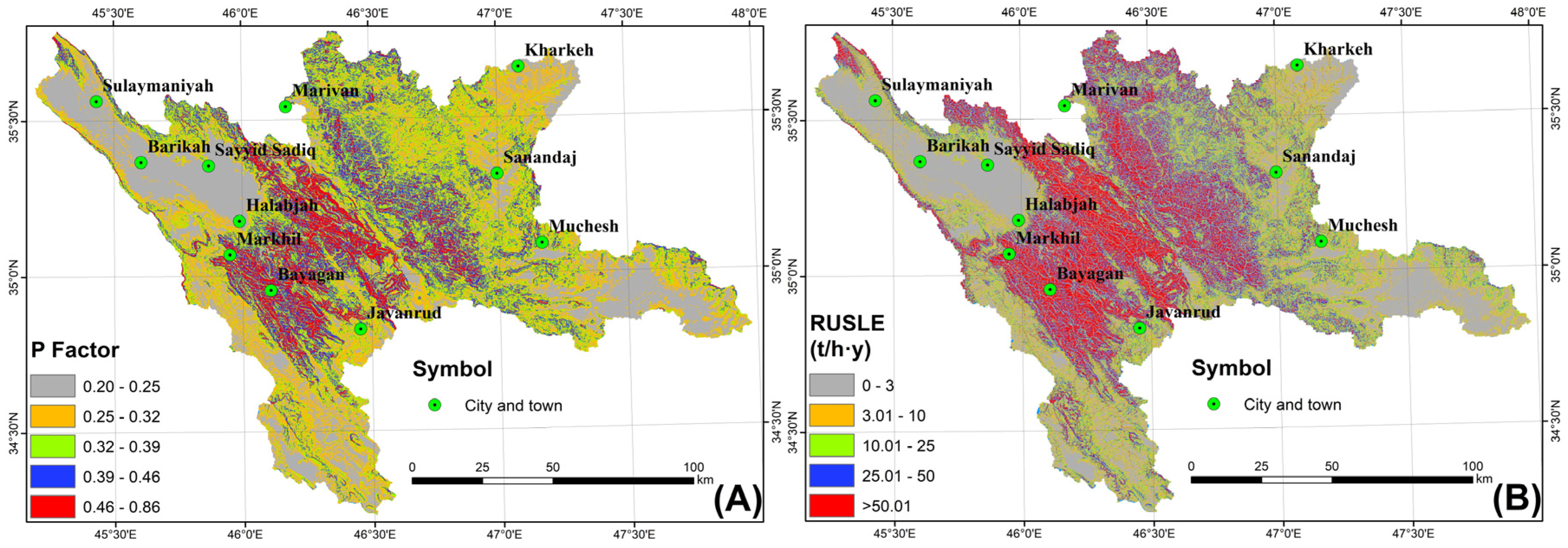
3.2.5. Support Practice (P Factor)
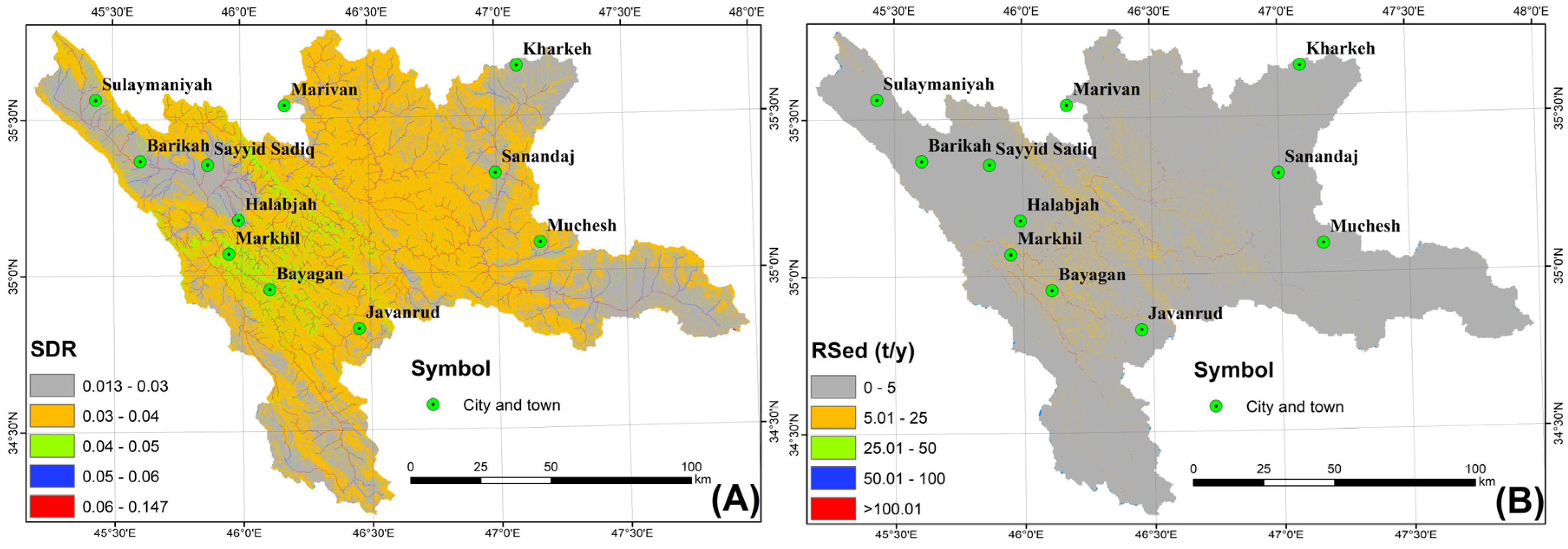
3.3. Sediment Delivery Ratio (SDR)

| α | β | References | Unit of the Area | Model No. |
|---|---|---|---|---|
| 0.4724 | 0.125 | [32,94,105] | km2 | SDR2 |
| 1.817 | 0.132 | [23,107] | km2 | SRD3 |
| 2.945 | 0.205 | [107] | km2 | SDR4 |
| 0.51 | 0.11 | [77,109,110] | mi2 | SDR5 |
3.4. Reservoir Sedimentation (RSed)
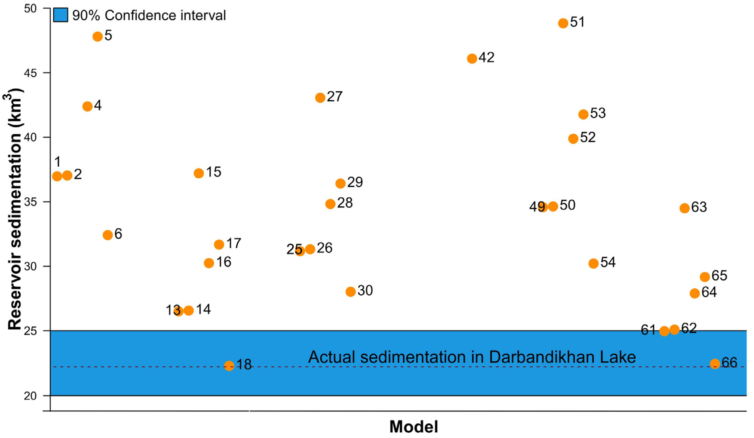
3.5. Validation
4. Results
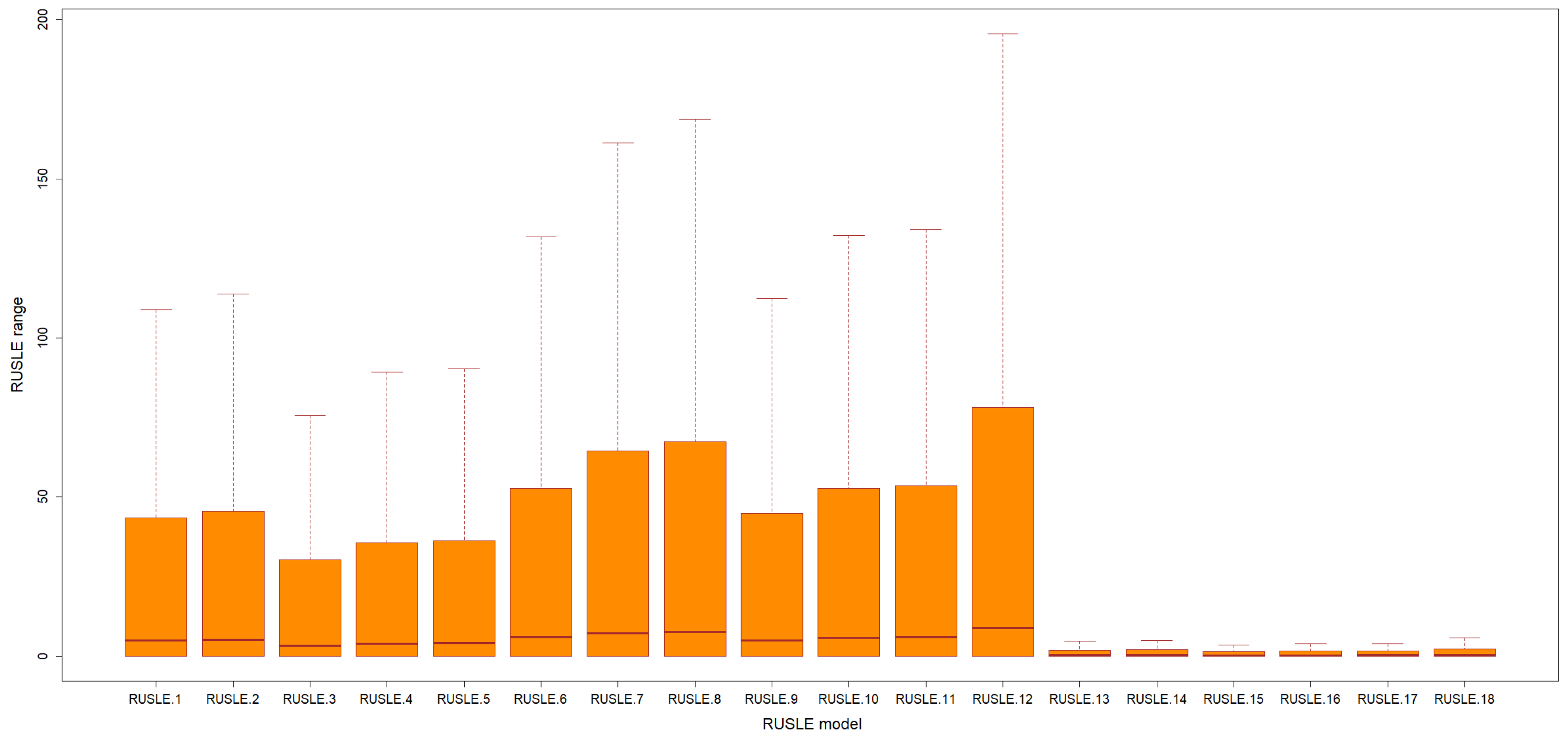
4.1. Estimation RUSLE and Its Factors
4.2. Sediment Delivery Ratio (DRr), Reservoir Sedimentation (RSed), and the Model Validation
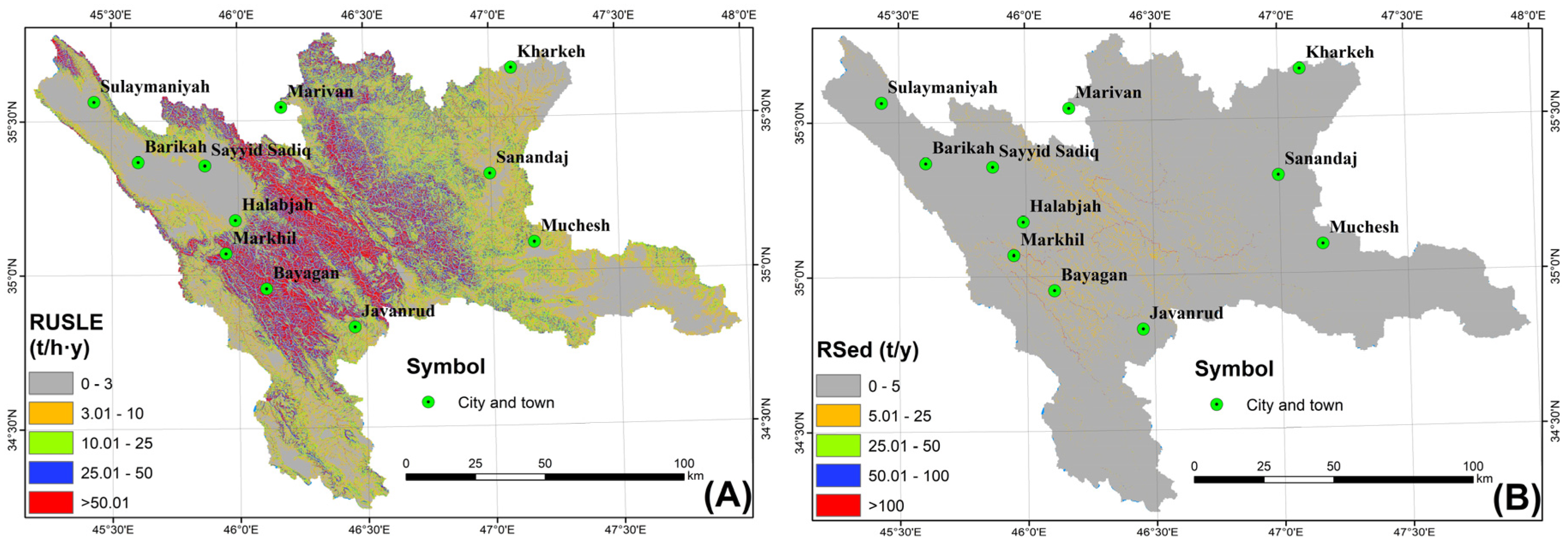
4.3. RUSLE, Its Factors, and Reservoir Sedimentation in the Present Day
5. Discussion
5.1. RUSLE-SDR and Its Factors
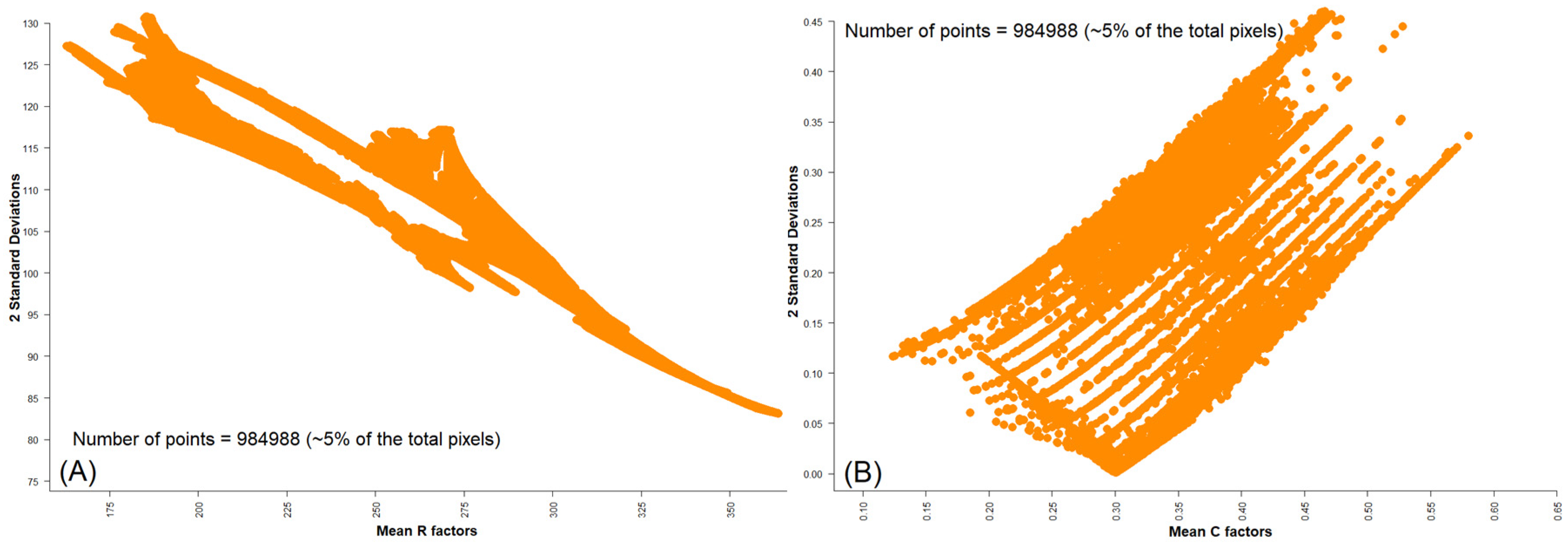
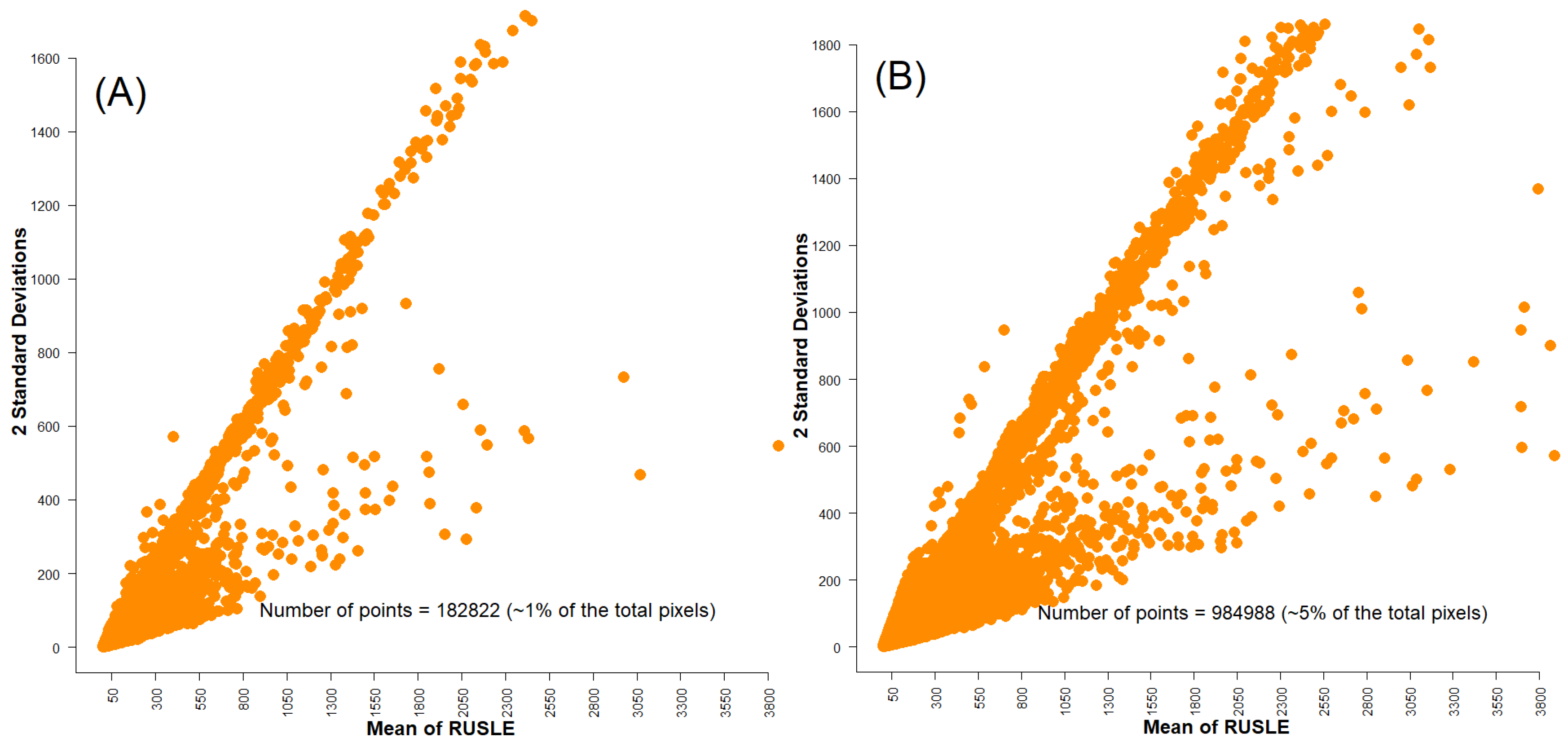
5.2. R Factor, C Factors, and RUSLE Uncertainties
5.3. Implications of This Study
6. Conclusions
Author Contributions
Funding
Data Availability Statement
Acknowledgments
Conflicts of Interest
Appendix A
| Scenarios | C-Equation | R-Equation | Scenarios | C-Equation | R-Equation |
|---|---|---|---|---|---|
| 1 | 18 | 3 | 10 | 17 | 6 |
| 2 | 18 | 4 | 11 | 17 | 7 |
| 3 | 18 | 5 | 12 | 17 | 8 |
| 4 | 18 | 6 | 13 | LC | 3 |
| 5 | 18 | 7 | 14 | LC | 4 |
| 6 | 18 | 8 | 15 | LC | 5 |
| 7 | 17 | 3 | 16 | LC | 6 |
| 8 | 17 | 4 | 17 | LC | 7 |
| 9 | 17 | 5 | 18 | LC | 8 |
Appendix B
| Elevation | VOLUME DIFF (MCM) | Elevation | VOLUME DIFF (MCM) | Elevation | VOLUME DIFF (MCM) | Elevation | VOLUME DIFF (MCM) |
|---|---|---|---|---|---|---|---|
| 434 | 186.5196177 | 449 | 368.2601237 | 464 | 454.2837 | 479 | 444.557 |
| 435 | 202.4116618 | 450 | 376.7507805 | 465 | 460.0191 | 480 | 454.4112 |
| 436 | 217.8700461 | 451 | 383.6461686 | 466 | 462.8374 | 481 | 446.2946 |
| 437 | 232.2080715 | 452 | 390.8162663 | 467 | 464.5166 | 482 | 434.6787 |
| 438 | 246.3789168 | 453 | 397.2368461 | 468 | 465.7219 | 483 | 435.0195 |
| 439 | 259.793523 | 454 | 402.6708382 | 469 | 467.6152 | 484 | 434.0626 |
| 440 | 273.5651565 | 455 | 408.1217914 | 470 | 468.8454 | 485 | 423.8966 |
| 441 | 285.4514375 | 456 | 412.3380251 | 471 | 469.2708 | 486 | 404.414 |
| 442 | 297.1203966 | 457 | 416.9450171 | 472 | 469.4618 | 487 | 368.7144 |
| 443 | 308.6056451 | 458 | 422.0896716 | 473 | 471.0426 | 488 | 323.7879 |
| 444 | 319.7122029 | 459 | 427.3771193 | 474 | 472.0941 | 489 | 267.4594 |
| 445 | 330.0812299 | 460 | 433.8615028 | 475 | 474.5954 | 490 | 209.1261 |
| 446 | 340.4472993 | 461 | 438.4430503 | 476 | 471.8698 | 491 | 145.1009 |
| 447 | 349.8499081 | 462 | 443.3719036 | 477 | 467.5566 | 492 | 59.9097 |
| 448 | 359.4951166 | 463 | 448.2591828 | 478 | 451.6446 | 493 | 0 |
Appendix C
| Scenarios | C Factor | R Factor | SDR | RSed (km3) | Error% | Scenarios | C Factor | R Factor | SDR | RSed (km3) | Error % |
|---|---|---|---|---|---|---|---|---|---|---|---|
| 1 | Equation (17) | Equation (7) | SDR1 | 36.96916 | 66.3554 | 46 | Land cover | Equation (3) | SDR5 | 5.181852 | 76.68248 |
| 2 | Equation (17) | Equation (6) | SDR1 | 37.03418 | 66.64798 | 47 | Land cover | Equation (4) | SDR5 | 5.417935 | 75.62015 |
| 3 | Equation (17) | Equation (8) | SDR1 | 52.05412 | 134.2353 | 48 | Land cover | Equation (5) | SDR5 | 4.169816 | 81.23648 |
| 4 | Equation (17) | Equation (3) | SDR1 | 42.38818 | 90.74013 | 49 | Equation (18) | Equation (7) | SDR5 | 34.57858 | 55.59816 |
| 5 | Equation (17) | Equation (4) | SDR1 | 47.80158 | 115.0996 | 50 | Equation (18) | Equation (6) | SDR5 | 34.63592 | 55.85619 |
| 6 | Equation (17) | Equation (5) | SDR1 | 32.41343 | 45.85533 | 51 | Equation (18) | Equation (8) | SDR5 | 48.8311 | 119.7323 |
| 7 | Land cover | Equation (7) | SDR1 | 3.045926 | 86.29381 | 52 | Equation (18) | Equation (3) | SDR5 | 39.88271 | 79.46591 |
| 8 | Land cover | Equation (6) | SDR1 | 3.062053 | 86.22124 | 53 | Equation (18) | Equation (4) | SDR5 | 41.76512 | 87.93646 |
| 9 | Land cover | Equation (8) | SDR1 | 4.221344 | 81.00462 | 54 | Equation (18) | Equation (5) | SDR5 | 30.20864 | 35.93412 |
| 10 | Land cover | Equation (3) | SDR1 | 3.415393 | 84.63127 | 55 | Equation (17) | Equation (7) | SDR4 | 287.1974 | 1192.343 |
| 11 | Land cover | Equation (4) | SDR1 | 3.575052 | 83.91283 | 56 | Equation (17) | Equation (6) | SDR4 | 287.0661 | 1191.752 |
| 12 | Land cover | Equation (5) | SDR1 | 2.718805 | 87.76581 | 57 | Equation (17) | Equation (8) | SDR4 | 409.8523 | 1744.271 |
| 13 | Equation (18) | Equation (7) | SDR1 | 26.49843 | 19.23876 | 58 | Equation (17) | Equation (3) | SDR4 | 336.9121 | 1416.051 |
| 14 | Equation (18) | Equation (6) | SDR1 | 26.56477 | 19.53728 | 59 | Equation (17) | Equation (4) | SDR4 | 352.692 | 1487.058 |
| 15 | Equation (18) | Equation (8) | SDR1 | 37.20219 | 67.404 | 60 | Equation (17) | Equation (5) | SDR4 | 248.1158 | 1016.482 |
| 16 | Equation (18) | Equation (3) | SDR1 | 30.24063 | 36.07807 | 61 | Land cover | Equation (7) | SDR4 | 24.96615 | 12.34374 |
| 17 | Equation (18) | Equation (4) | SDR1 | 31.67841 | 42.54786 | 62 | Land cover | Equation (6) | SDR4 | 25.08741 | 12.88939 |
| 18 | Equation (18) | Equation (5) | SDR1 | 22.29416 | 0.320209 | 63 | Land cover | Equation (8) | SDR4 | 34.49158 | 55.20668 |
| 19 | Equation (17) | Equation (7) | SDR3 | 358.5325 | 1513.34 | 64 | Land cover | Equation (3) | SDR4 | 27.89489 | 25.52261 |
| 20 | Equation (17) | Equation (6) | SDR3 | 358.3681 | 1512.6 | 65 | Land cover | Equation (4) | SDR4 | 29.16574 | 31.24124 |
| 21 | Equation (17) | Equation (8) | SDR3 | 511.6561 | 2202.372 | 66 | Land cover | Equation (5) | SDR4 | 22.44697 | 1.00783 |
| 22 | Equation (17) | Equation (3) | SDR3 | 420.5986 | 1792.627 | 67 | Equation (18) | Equation (7) | SDR4 | 186.1391 | 737.5966 |
| 23 | Equation (17) | Equation (4) | SDR3 | 440.2978 | 1881.271 | 68 | Equation (18) | Equation (6) | SDR4 | 186.4481 | 738.9871 |
| 24 | Equation (17) | Equation (5) | SDR3 | 309.742 | 1293.79 | 69 | Equation (18) | Equation (8) | SDR4 | 262.8601 | 1082.829 |
| 25 | Land cover | Equation (7) | SDR3 | 31.16664 | 40.24497 | 70 | Equation (18) | Equation (3) | SDR4 | 214.6905 | 866.0734 |
| 26 | Land cover | Equation (6) | SDR3 | 31.31803 | 40.9262 | 71 | Equation (18) | Equation (4) | SDR4 | 224.8236 | 911.6708 |
| 27 | Land cover | Equation (8) | SDR3 | 43.05787 | 93.75363 | 72 | Equation (18) | Equation (5) | SDR4 | 162.6163 | 631.7477 |
| 28 | Land cover | Equation (3) | SDR3 | 34.82278 | 56.69703 | 73 | Equation (17) | Equation (7) | SDR2 | 99.73186 | 348.7777 |
| 29 | Land cover | Equation (4) | SDR3 | 36.40928 | 63.83603 | 74 | Equation (17) | Equation (6) | SDR2 | 99.6861 | 348.5717 |
| 30 | Land cover | Equation (5) | SDR3 | 28.02177 | 26.09355 | 75 | Equation (17) | Equation (8) | SDR2 | 142.3258 | 540.4437 |
| 31 | Equation (18) | Equation (7) | SDR3 | 232.3718 | 945.6365 | 76 | Equation (17) | Equation (3) | SDR2 | 116.9967 | 426.4667 |
| 32 | Equation (18) | Equation (6) | SDR3 | 232.7572 | 947.3707 | 77 | Equation (17) | Equation (4) | SDR2 | 122.4763 | 451.1241 |
| 33 | Equation (18) | Equation (8) | SDR3 | 328.1499 | 1376.623 | 78 | Equation (17) | Equation (5) | SDR2 | 86.1599 | 287.706 |
| 34 | Equation (18) | Equation (3) | SDR3 | 268.0158 | 1106.029 | 79 | Land cover | Equation (7) | SDR2 | 8.669506 | 60.98859 |
| 35 | Equation (18) | Equation (4) | SDR3 | 280.6658 | 1162.952 | 80 | Land cover | Equation (6) | SDR2 | 8.711617 | 60.7991 |
| 36 | Equation (18) | Equation (5) | SDR3 | 203.0056 | 813.4932 | 81 | Land cover | Equation (8) | SDR2 | 11.97725 | 46.10426 |
| 37 | Equation (17) | Equation (7) | SDR5 | 53.35229 | 140.0769 | 82 | Land cover | Equation (3) | SDR2 | 9.686521 | 56.41218 |
| 38 | Equation (17) | Equation (6) | SDR5 | 53.3278 | 139.9667 | 83 | Land cover | Equation (4) | SDR2 | 10.12783 | 54.42636 |
| 39 | Equation (17) | Equation (8) | SDR5 | 76.13834 | 242.6105 | 84 | Land cover | Equation (5) | SDR2 | 7.794709 | 64.92504 |
| 40 | Equation (17) | Equation (3) | SDR5 | 62.58831 | 181.6375 | 85 | Equation (18) | Equation (7) | SDR2 | 64.63809 | 190.8612 |
| 41 | Equation (17) | Equation (4) | SDR5 | 65.5197 | 194.8283 | 86 | Equation (18) | Equation (6) | SDR2 | 64.74529 | 191.3436 |
| 42 | Equation (17) | Equation (5) | SDR5 | 46.09182 | 107.4059 | 87 | Equation (18) | Equation (8) | SDR2 | 91.28039 | 310.7474 |
| 43 | Land cover | Equation (7) | SDR5 | 4.637795 | 79.13065 | 88 | Equation (18) | Equation (3) | SDR2 | 74.55308 | 235.4771 |
| 44 | Land cover | Equation (6) | SDR5 | 4.660323 | 79.02928 | 89 | Equation (18) | Equation (4) | SDR2 | 78.07189 | 251.3112 |
| 45 | Land cover | Equation (8) | SDR5 | 6.40729 | 71.1682 | 90 | Equation (18) | Equation (5) | SDR2 | 56.46937 | 154.1033 |
References
- Hajigholizadeh, M.; Melesse, A.M.; Fuentes, H.R. Erosion and Sediment Transport Modelling in Shallow Waters: A Review on Approaches, Models and Applications. Int. J. Environ. Res. Public Health 2018, 15, 518. [Google Scholar] [CrossRef] [PubMed] [Green Version]
- Alewell, C.; Borrelli, P.; Meusburger, K.; Panagos, P. Using the USLE: Chances, challenges and limitations of soil erosion modelling. Int. Soil Water Conserv. Res. 2019, 7, 203–225. [Google Scholar] [CrossRef]
- Kuznetsov, M.; Gendugov, V.; Khalilov, M.; Ivanuta, A. An equation of soil detachment by flow. Soil Tillage Res. 1998, 46, 97–102. [Google Scholar] [CrossRef]
- Pal, S. Identification of soil erosion vulnerable areas in Chandrabhaga river basin: A multi-criteria decision approach. Model. Earth Syst. Environ. 2016, 2, 5. [Google Scholar] [CrossRef] [Green Version]
- Walling, D.E. The Impact of Global Change on Erosion and Sediment Transport by Rivers: Current Progress and Future Challenges; UNESCO: London, UK, 2009. [Google Scholar]
- Hamel, P.; Chaplin-Kramer, R.; Sim, S.; Mueller, C. A new approach to modeling the sediment retention service (InVEST 3.0): Case study of the Cape Fear catchment, North Carolina, USA. Sci. Total. Environ. 2015, 524-525, 166–177. [Google Scholar] [CrossRef]
- Toy, T.J.; Foster, G.R.; Renard, K.G. Soil Erosion: Processes, Prediction, Measurement, and Control; Wiley: New York, NY, USA, 2002; ISBN 9780471383697. [Google Scholar]
- Montanarella, L.; Pennock, D.J.; McKenzie, N.; Badraoui, M.; Chude, V.; Baptista, I.; Mamo, T.; Yemefack, M.; Aulakh, M.S.; Yagi, K.; et al. World’s soils are under threat. Soild 2015, 2, 1263–1272. [Google Scholar] [CrossRef] [Green Version]
- Patro, E.R.; De Michele, C.; Granata, G.; Biagini, C. Assessment of current reservoir sedimentation rate and storage capacity loss: An Italian overview. J. Environ. Manag. 2022, 320, 115826. [Google Scholar] [CrossRef]
- World Commission on Dams. Dams and Development. A New Framework for Decision-Making. The Report of the World Commission on Dams; Earthscan: Oxford, UK, 2000. [Google Scholar]
- Cogollo, P.R.J.; Villela, S.M. Mathematical Model for Reservoir Silting. Sediment Budg. 1988, 174, 43–52. [Google Scholar]
- Rajbanshi, J.; Bhattacharya, S. Assessment of soil erosion, sediment yield and basin specific controlling factors using RUSLE-SDR and PLSR approach in Konar river basin, India. J. Hydrol. 2020, 587, 124935. [Google Scholar] [CrossRef]
- Majhi, A.; Shaw, R.; Mallick, K.; Patel, P.P. Towards improved USLE-based soil erosion modelling in India: A review of prevalent pitfalls and implementation of exemplar methods. Earth-Science Rev. 2021, 221, 103786. [Google Scholar] [CrossRef]
- Renard, K.G.; Foster, G.R.; Weesies, G.A.; McCool, D.K.; Yoder, D.C. Predicting Soil Erosion by Water: A Guide to Conservation Planning with the Revised Universal Soil Loss Equation (RUSLE); United States Department of Agriculture: Washington, DC, USA, 1997; Volume 703.
- Wischmeier, W.H.; Smith, D.D. Predicting Rainfall Erosion Losses: A Guide to Conservation Planning [USA]; Agriculture Handbook; United States Department of Agriculture: Washington, DC, USA, 1978.
- Brychta, J.; Podhrázská, J.; Šťastná, M. Review of methods of spatio-temporal evaluation of rainfall erosivity and their correct application. Catena 2022, 217, 106454. [Google Scholar] [CrossRef]
- Karan, S.K.; Ghosh, S.; Samadder, S.R. Identification of spatially distributed hotspots for soil loss and erosion potential in mining areas of Upper Damodar Basin—India. Catena 2019, 182, 104144. [Google Scholar] [CrossRef]
- Sonneveld, B.; Nearing, M. A nonparametric/parametric analysis of the Universal Soil Loss Equation. Catena 2003, 52, 9–21. [Google Scholar] [CrossRef] [Green Version]
- Cao, X.; Hu, X.; Han, M.; Jin, T.; Yang, X.; Yang, Y.; He, K.; Wang, Y.; Huang, J.; Xi, C.; et al. Characteristics and predictive models of hillslope erosion in burned areas in Xichang, China, on March 30, 2020. Catena 2022, 217, 106509. [Google Scholar] [CrossRef]
- Lu, H.; Moran, C.; Prosser, I.P. Modelling sediment delivery ratio over the Murray Darling Basin. Environ. Model. Softw. 2006, 21, 1297–1308. [Google Scholar] [CrossRef]
- Vigiak, O.; Borselli, L.; Newham, L.; McInnes, J.; Roberts, A. Comparison of conceptual landscape metrics to define hillslope-scale sediment delivery ratio. Geomorphology 2012, 138, 74–88. [Google Scholar] [CrossRef]
- Borselli, L.; Cassi, P.; Torri, D. Prolegomena to sediment and flow connectivity in the landscape: A GIS and field numerical assessment. Catena 2008, 75, 268–277. [Google Scholar] [CrossRef]
- Othman, A.A.; Obaid, A.K.; Al-Manmi, D.A.M.A.; Al-Maamar, A.F.; Hasan, S.E.; Liesenberg, V.; Shihab, A.T.; Al-Saady, Y.I. New Insight on Soil Loss Estimation in the Northwestern Region of the Zagros Fold and Thrust Belt. ISPRS Int. J. Geo-Inf. 2021, 10, 59. [Google Scholar] [CrossRef]
- Othman, A.A.; Obaid, A.K.; Sissakian, V.K.; Maamar, A.F.A.; Shihab, A.T. RUSLE Model in the Northwest Part of the Zagros Mountain Belt BT—Environmental Degradation in Asia: Land Degradation, Environmental Contamination, and Human Activities; Al-Quraishi, A.M.F., Mustafa, Y.T., Negm, A.M., Eds.; Springer International Publishing: Cham, Switzerland, 2022; pp. 287–306. ISBN 978-3-031-12112-8. [Google Scholar]
- Allafta, H.; Opp, C. Soil Erosion Assessment Using the RUSLE Model, Remote Sensing, and GIS in the Shatt Al-Arab Basin (Iraq-Iran). Appl. Sci. 2022, 12, 7776. [Google Scholar] [CrossRef]
- Al-Abadi, A.M.A.; Ghalib, H.B.; Al-Qurnawi, W.S. Estimation of Soil Erosion in Northern Kirkuk Governorate, Iraq Using Rusle, Remote Sensing and Gis. Carpathian J. Earth Environ. Sci. 2016, 11, 153–166. [Google Scholar]
- Bayazıt, Y.; Koç, C. The impact of forest fires on floods and erosion: Marmaris, Turkey. Environ. Dev. Sustain. 2022, 24, 13426–13445. [Google Scholar] [CrossRef]
- Imamoglu, A.; Dengiz, O. Determination of soil erosion risk using RUSLE model and soil organic carbon loss in Alaca catchment (Central Black Sea region, Turkey). Rend. Lincei 2017, 28, 11–23. [Google Scholar] [CrossRef]
- Ustaoğlu, B.; Ikiel, C.; Dutucu, A.A.; Koç, D.E. Erosion Susceptibility Analysis in Datça and Bozburun Peninsulas, Turkey. Iran. J. Sci. Technol. Trans. A Sci. 2021, 45, 557–570. [Google Scholar] [CrossRef]
- Sarp, G. Interaction between sediment transport rate and tectonic activity: The case of Kızılırmak Basin on the tectonically active NAFZ, Turkey. Arab. J. Geosci. 2020, 13, 265. [Google Scholar] [CrossRef]
- Irvem, A.; Topaloğlu, F.; Uygur, V. Estimating spatial distribution of soil loss over Seyhan River Basin in Turkey. J. Hydrol. 2007, 336, 30–37. [Google Scholar] [CrossRef]
- Ozsoy, G.; Aksoy, E.; Dirim, M.S.; Tumsavas, Z. Determination of Soil Erosion Risk in the Mustafakemalpasa River Basin, Turkey, Using the Revised Universal Soil Loss Equation, Geographic Information System, and Remote Sensing. Environ. Manag. 2012, 50, 679–694. [Google Scholar] [CrossRef]
- Ozsoy, G.; Aksoy, E. Estimation of soil erosion risk within an important agricultural sub-watershed in Bursa, Turkey, in relation to rapid urbanization. Environ. Monit. Assess. 2015, 187, 419. [Google Scholar] [CrossRef]
- Akbarzadeh, A.; Ghorbani-Dashtaki, S.; Naderi-Khorasgani, M.; Kerry, R.; Taghizadeh-Mehrjardi, R. Monitoring and assessment of soil erosion at micro-scale and macro-scale in forests affected by fire damage in northern Iran. Environ. Monit. Assess. 2016, 188, 699. [Google Scholar] [CrossRef]
- Arekhi, S.; Niazi, Y.; Kalteh, A.M. Soil erosion and sediment yield modeling using RS and GIS techniques: A case study, Iran. Arab. J. Geosci. 2012, 5, 285–296. [Google Scholar] [CrossRef]
- Fallah, M.; Kavian, A.; Omidvar, E. Watershed prioritization in order to implement soil and water conservation practices. Environ. Earth Sci. 2016, 75, 1248. [Google Scholar] [CrossRef]
- Vaezi, A.R.; Sadeghi, S.H.R. Evaluating the RUSLE model and developing an empirical equation for estimating soil erodibility factor in a semi-arid region. Span. J. Agric. Res. 2011, 9, 912. [Google Scholar] [CrossRef] [Green Version]
- Mirghaed, F.A.; Souri, B.; Mohammadzadeh, M.; Salmanmahiny, A.; Mirkarimi, S.H. Evaluation of the relationship between soil erosion and landscape metrics across Gorgan Watershed in northern Iran. Environ. Monit. Assess. 2018, 190, 643. [Google Scholar] [CrossRef]
- Mirakhorlo, M.S.; Rahimzadegan, M. Evaluating estimated sediment delivery by Revised Universal Soil Loss Equation (RUSLE) and Sediment Delivery Distributed (SEDD) in the Talar Watershed, Iran. Front. Earth Sci. 2020, 14, 50–62. [Google Scholar] [CrossRef]
- Zare, M.; Samani, A.A.N.; Mohammady, M.; Salmani, H.; Bazrafshan, J. Investigating effects of land use change scenarios on soil erosion using CLUE-s and RUSLE models. Int. J. Environ. Sci. Technol. 2017, 14, 1905–1918. [Google Scholar] [CrossRef]
- Zare, M.; Samani, A.A.N.; Mohammady, M.; Teimurian, T.; Bazrafshan, J. Simulation of soil erosion under the influence of climate change scenarios. Environ. Earth Sci. 2016, 75, 1405. [Google Scholar] [CrossRef]
- Ebrahimzadeh, S.; Motagh, M.; Mahboub, V.; Harijani, F.M. An improved RUSLE/SDR model for the evaluation of soil erosion. Environ. Earth Sci. 2018, 77, 454. [Google Scholar] [CrossRef]
- Avand, M.; Mohammadi, M.; Mirchooli, F.; Kavian, A.; Tiefenbacher, J.P. A New Approach for Smart Soil Erosion Modeling: Integration of Empirical and Machine-Learning Models. Environ. Model. Assess. 2022, 28, 145–160. [Google Scholar] [CrossRef]
- Damaneh, H.E.; Khosravi, H.; Habashi, K.; Tiefenbacher, J.P. The impact of land use and land cover changes on soil erosion in western Iran. Nat. Hazards 2022, 110, 2185–2205. [Google Scholar] [CrossRef]
- Zakeri, E.; Mousavi, S.A.; Karimzadeh, H. Scenario-based modelling of soil conservation function by rangeland vegetation cover in northeastern Iran. Environ. Earth Sci. 2020, 79, 107. [Google Scholar] [CrossRef]
- Mehri, A.; Salmanmahiny, A.; Tabrizi, A.R.M.; Mirkarimi, S.H.; Sadoddin, A. Investigation of likely effects of land use planning on reduction of soil erosion rate in river basins: Case study of the Gharesoo River Basin. Catena 2018, 167, 116–129. [Google Scholar] [CrossRef]
- Azari, M.; Oliaye, A.; Nearing, M.A. Expected climate change impacts on rainfall erosivity over Iran based on CMIP5 climate models. J. Hydrol. 2021, 593, 125826. [Google Scholar] [CrossRef]
- Derakhshan-Babaei, F.; Nosrati, K.; Mirghaed, F.A.; Egli, M. The interrelation between landform, land-use, erosion and soil quality in the Kan catchment of the Tehran province, central Iran. Catena 2021, 204, 105412. [Google Scholar] [CrossRef]
- Doulabian, S.; Toosi, A.S.; Calbimonte, G.H.; Tousi, E.G.; Alaghmand, S. Projected climate change impacts on soil erosion over Iran. J. Hydrol. 2021, 598, 126432. [Google Scholar] [CrossRef]
- Ostovari, Y.; Ghorbani-Dashtaki, S.; Kumar, L.; Shabani, F. Soil erodibility and its prediction in semi-arid regions. Arch. Agron. Soil Sci. 2019, 65, 1688–1703. [Google Scholar] [CrossRef]
- General Directorate of Research Agricultural Extension. Climate Data; Ministry of Agriculture of the Kurdistan Regional: Sulaimaniyah, Iraq, 2020. [Google Scholar]
- Yousif, O.S.Q.; Zaidn, K.; Alshkane, Y.; Khani, A.; Hama, S. Performance of Darbandikhan Dam during a Major Earthquake on November 12, 2017. In Proceedings of the EWG2019, 3rd Meeting of Dams and Earthquakes, An International Symposium, Lisbon, Portugal, 6–8 May 2019; pp. 295–308. [Google Scholar]
- Strahler, A.N. Quantitative analysis of watershed geomorphology. Eos Trans. Am. Geophys. Union 1957, 38, 913–920. [Google Scholar] [CrossRef] [Green Version]
- Saleh, D.K. Stream Gage Descriptions and Streamflow Statistics for Sites in the Tigris River and Euphrates River Basins, Iraq; U.S. Geological Survey: Reston, VA, USA, 2010. [Google Scholar] [CrossRef]
- Amini, A.; Bahrami, J.; Miraki, A. Effects of dam break on downstream dam and lands using GIS and Hec Ras: A decision basis for the safe operation of two successive dams. Int. J. River Basin Manag. 2021, 20, 487–498. [Google Scholar] [CrossRef]
- Rashidi, M.; Haeri, S.M. Evaluation of behaviors of earth and rockfill dams during construction and initial impounding using instrumentation data and numerical modeling. J. Rock Mech. Geotech. Eng. 2017, 9, 709–725. [Google Scholar] [CrossRef]
- Faraj, D.M.; Zaidan, K. The Impact of the Tropical Water Project on Darbandikhan Dam and Diyala River Basin. Iraqi J. Civ. Eng. 2022, 14, 1–6. [Google Scholar]
- Hosseini, S.P.; Jafari, R.; Esfahani, M.T.; Senn, J.; Hemami, M.-R.; Amiri, M. Investigating habitat degradation of Ursus arctos using species distribution modelling and remote sensing in Zagros Mountains of Iran. Arab. J. Geosci. 2021, 14, 2179. [Google Scholar] [CrossRef]
- Rabus, B.; Eineder, M.; Roth, A.; Bamler, R. The shuttle radar topography mission—A new class of digital elevation models acquired by spaceborne radar. ISPRS J. Photogramm. Remote Sens. 2003, 57, 241–262. [Google Scholar] [CrossRef]
- GSFC_DAAC. Tropical Rainfall Measurement Mission Project (TRMM; 3B43 V7). Available online: https://disc.gsfc.nasa.gov/datasets/TRMM_3B43_7/summary (accessed on 14 January 2023).
- Kummerow, C.; Barnes, W.; Kozu, T.; Shiue, J.; Simpson, J. The Tropical Rainfall Measuring Mission (TRMM) Sensor Package. J. Atmos. Ocean. Technol. 1998, 15, 809–817. [Google Scholar] [CrossRef]
- Nachtergaele, F.; van Velthuizen, H.; van Engelen, V.; Fischer, G.; Jones, A.; Montanarella, L.; Petri, M.; Prieler, S.; Teixeira, E.; Shi, X. Harmonized World Soil Database, version 1.2; FAO: Rome, Italy; IIASA: Laxenburg, Austria, 2012; pp. 1–50. [Google Scholar]
- Jenkerson, C.; Maiersperger, T.; Schmidt, G. EMODIS: A User-Friendly Data Source; U.S. Geological Survey: Reston, VA, USA, 2010.
- Almagro, A.; Thomé, T.C.; Colman, C.B.; Pereira, R.B.; Junior, J.M.; Rodrigues, D.B.B.; Oliveira, P.T.S. Improving cover and management factor (C-factor) estimation using remote sensing approaches for tropical regions. Int. Soil Water Conserv. Res. 2019, 7, 325–334. [Google Scholar] [CrossRef]
- NASA. User Guide for the MODIS Land Cover Type Product (MCD12Q1). 2013. Available online: https://lpdaac.usgs.gov/documents/438/MCD12Q1_User_Guide_V51.pdf (accessed on 14 January 2023).
- Wan, Z.; Zhang, Y.; Zhang, Q.; Li, Z.L. Validation of the land-surface temperature products retrieved from Terra Moderate Resolution Imaging Spectroradiometer data. Remote Sens. Environ. 2002, 83, 163–180. [Google Scholar] [CrossRef]
- Lina, H.; Wanga, J.; Jia, X.; Bo, Y.; Wang, D.; Wang, Z. Evaluation of Modis Land Cover Product of East China. In Proceedings of the International Geoscience and Remote Sensing Symposium (IGARSS), Boston, MA, USA, 8–11 July 2008; Volume 4, pp. IV762–IV765. [Google Scholar]
- ESRI. ArcGIS Desktop: Release 10.8; ESRI: Redlands, CA, USA, 2021. [Google Scholar]
- Cavalli, M.; Trevisani, S.; Comiti, F.; Marchi, L. Geomorphometric assessment of spatial sediment connectivity in small Alpine catchments. Geomorphology 2013, 188, 31–41. [Google Scholar] [CrossRef]
- Shahzad, F.; Gloaguen, R. TecDEM: A MATLAB based toolbox for tectonic geomorphology, Part 1: Drainage network preprocessing and stream profile analysis. Comput. Geosci. 2011, 37, 250–260. [Google Scholar] [CrossRef]
- R_Core_Team. R: A Language and Environment for Statistical Computing; R Foundation for Statistical Computing: Vienna, Austria, 2022. [Google Scholar]
- da Cunha, E.R.; Santos, C.A.G.; da Silva, R.M.; Panachuki, E.; de Oliveira, P.T.S.; Oliveira, N.D.S.; Falcão, K.D.S. Assessment of current and future land use/cover changes in soil erosion in the Rio da Prata basin (Brazil). Sci. Total. Environ. 2022, 818, 151811. [Google Scholar] [CrossRef]
- Panagos, P.; Meusburger, K.; Ballabio, C.; Borrelli, P.; Alewell, C. Soil erodibility in Europe: A high-resolution dataset based on LUCAS. Sci. Total Environ. 2014, 479–480, 189–200. [Google Scholar] [CrossRef]
- Renard, K.G.; Foster, G.R.; Weesies, G.A.; Porter, J.P. RUSLE: Revised Universal Soil Loss Equation. J. Soil Water Conserv. 1991, 46, 30–33. [Google Scholar]
- Sun, W.; Shao, Q.; Liu, J.; Zhai, J. Assessing the effects of land use and topography on soil erosion on the Loess Plateau in China. Catena 2014, 121, 151–163. [Google Scholar] [CrossRef]
- Kayet, N.; Pathak, K.; Chakrabarty, A.; Sahoo, S. Evaluation of soil loss estimation using the RUSLE model and SCS-CN method in hillslope mining areas. Int. Soil Water Conserv. Res. 2018, 6, 31–42. [Google Scholar] [CrossRef]
- Rosas, M.A.; Gutierrez, R.R. Assessing soil erosion risk at national scale in developing countries: The technical challenges, a proposed methodology, and a case history. Sci. Total. Environ. 2020, 703, 135474. [Google Scholar] [CrossRef] [PubMed]
- Salar, S.G.; Othman, A.A.; Rasooli, S.; Ali, S.S.; Al-Attar, Z.T.; Liesenberg, V. GIS-Based Modeling for Vegetated Land Fire Prediction in Qaradagh Area, Kurdistan Region, Iraq. Sustainability 2022, 14, 6194. [Google Scholar] [CrossRef]
- Othman, A.A.; Al-Maamar, A.F.; Al-Manmi, D.A.M.; Veraldo, L.; Hasan, S.E.; Obaid, A.K.; Al-Quraishi, A.M.F. GIS-Based Modeling for Selection of Dam Sites in the Kurdistan Region, Iraq. ISPRS Int. J. Geo-Inf. 2020, 9, 244. [Google Scholar] [CrossRef]
- Salar, S.G.; Othman, A.A.; Hasan, S.E. Identification of suitable sites for groundwater recharge in Awaspi watershed using GIS and remote sensing techniques. Environ. Earth Sci. 2018, 77, 701. [Google Scholar] [CrossRef]
- Renard, K.G.; Freimund, J.R. Using monthly precipitation data to estimate the R-factor in the revised USLE. J. Hydrol. 1994, 157, 287–306. [Google Scholar] [CrossRef]
- Arnoldus, H.M.J. An Approximation of the Rainfall Factor in the Universal Soil Loss Equation. In Assessment of Erosion; John Wiley and Sons: New York, NY, USA, 1980; pp. 127–132. [Google Scholar]
- Ostovari, Y.; Ghorbani-Dashtaki, S.; Bahrami, H.-A.; Naderi, M.; Dematte, J.A.M. Soil loss estimation using RUSLE model, GIS and remote sensing techniques: A case study from the Dembecha Watershed, Northwestern Ethiopia. Geoderma Reg. 2017, 11, 28–36. [Google Scholar] [CrossRef]
- Sadeghi, S.H.R.; Moatamednia, M.; Behzadfar, M. Spatial and Temporal Variations in the Rainfall Erosivity Factor in Iran TT. Journal of Agricultural Science and Technology 2011, 13, 451–464. [Google Scholar]
- Zabihi, M.; Sadeghi, S.H.; Vafakhah, M. Spatial Analysis of Rainfall Erosivity Index Patterns at Different Time Scales in Iran. Watershed Eng. Manag. 2015, 7, 442–457. [Google Scholar]
- Phinzi, K.; Ngetar, N.S. The assessment of water-borne erosion at catchment level using GIS-based RUSLE and remote sensing: A review. Int. Soil Water Conserv. Res. 2019, 7, 27–46. [Google Scholar] [CrossRef]
- Zerihun, M.; Mohammedyasin, M.S.; Sewnet, D.; Adem, A.A.; Lakew, M. Assessment of soil erosion using RUSLE, GIS and remote sensing in NW Ethiopia. Geoderma Reg. 2018, 12, 83–90. [Google Scholar] [CrossRef]
- Ijaz, M.A.; Ashraf, M.; Hamid, S.; Niaz, Y.; Waqas, M.M.; Tariq, M.A.U.R.; Saifullah, M.; Bhatti, M.T.; Tahir, A.A.; Ikram, K.; et al. Prediction of Sediment Yield in a Data-Scarce River Catchment at the Sub-Basin Scale Using Gridded Precipitation Datasets. Water 2022, 14, 1480. [Google Scholar] [CrossRef]
- Ali, M.G.; Ali, S.; Arshad, R.H.; Nazeer, A.; Waqas, M.M.; Waseem, M.; Aslam, R.A.; Cheema, M.J.M.; Leta, M.K.; Shauket, I. Estimation of Potential Soil Erosion and Sediment Yield: A Case Study of the Transboundary Chenab River Catchment. Water 2021, 13, 3647. [Google Scholar] [CrossRef]
- Kerven, G.L.; Menzies, N.; Geyer, M.D. Analytical methods and quality assurance. Commun. Soil Sci. Plant Anal. 2000, 31, 1935–1939. [Google Scholar] [CrossRef]
- Moore, I.D.; Burch, G.J. Physical Basis of the Length-slope Factor in the Universal Soil Loss Equation. Soil Sci. Soc. Am. J. 1986, 50, 1294–1298. [Google Scholar] [CrossRef]
- Li, Y.; Qi, S.; Liang, B.; Ma, J.; Cheng, B.; Ma, C.; Qiu, Y.; Chen, Q. Dangerous degree forecast of soil loss on highway slopes in mountainous areas of the Yunnan–Guizhou Plateau (China) using the Revised Universal Soil Loss Equation. Nat. Hazards Earth Syst. Sci. 2019, 19, 757–774. [Google Scholar] [CrossRef]
- Van der Knijff, J.M.; Jones, R.J.A.; Montanarella, L. Soil Erosion Risk: Assessment in Europe; European Commission: Brussels, Belgium, 2000. [Google Scholar]
- Ozsoy, G.; Aksoy, E. Prediction of soil loss differences and sediment accumulation at the Nilufer creek watershed, Turkey, using multiyear satellite data in a GIS. Geocarto Int. 2015, 30, 843–857. [Google Scholar] [CrossRef]
- Lin, C.-Y. A Study on the Width and Placement of Vegetated Buffer Strips in a Mudstone-Distributed Watershed. J. China Soil Water Conserv. 1997, 29, 250–266. [Google Scholar]
- Woznicki, S.A.; Cada, P.; Wickham, J.; Schmidt, M.; Baynes, J.; Mehaffey, M.; Neale, A. Sediment retention by natural landscapes in the conterminous United States. Sci. Total Environ. 2020, 745, 140972. [Google Scholar] [CrossRef]
- Xu, Z.; Zhang, S.; Zhou, Y.; Hou, X.; Yang, X. Characteristics of watershed dynamic sediment delivery based on improved RUSLE model. Catena 2022, 219, 106602. [Google Scholar] [CrossRef]
- Chuenchum, P.; Xu, M.; Tang, W. Estimation of Soil Erosion and Sediment Yield in the Lancang–Mekong River Using the Modified Revised Universal Soil Loss Equation and GIS Techniques. Water 2020, 12, 135. [Google Scholar] [CrossRef] [Green Version]
- Benavidez, R.; Jackson, B.; Maxwell, D.; Norton, K. A review of the (Revised) Universal Soil Loss Equation ((R)USLE): With a view to increasing its global applicability and improving soil loss estimates. Hydrol. Earth Syst. Sci. 2018, 22, 6059–6086. [Google Scholar] [CrossRef] [Green Version]
- Yigez, B.; Xiong, D.; Zhang, B.; Yuan, Y.; Baig, M.A.; Dahal, N.M.; Guadie, A.; Zhao, W.; Wu, Y. Spatial distribution of soil erosion and sediment yield in the Koshi River Basin, Nepal: A case study of Triyuga watershed. J. Soils Sediments 2021, 21, 3888–3905. [Google Scholar] [CrossRef]
- Durigon, V.L.; de Carvalho, D.F.; Antunes, M.A.H.; Oliveira, P.T.; Fernandes, M.M. NDVI time series for monitoring RUSLE cover management factor in a tropical watershed. Int. J. Remote Sens. 2014, 35, 441–453. [Google Scholar] [CrossRef]
- Bakker, M.M.; Govers, G.; van Doorn, A.; Quetier, F.; Chouvardas, D.; Rounsevell, M. The response of soil erosion and sediment export to land-use change in four areas of Europe: The importance of landscape pattern. Geomorphology 2008, 98, 213–226. [Google Scholar] [CrossRef]
- Terranova, O.; Antronico, L.; Coscarelli, R.; Iaquinta, P. Soil erosion risk scenarios in the Mediterranean environment using RUSLE and GIS: An application model for Calabria (southern Italy). Geomorphology 2009, 112, 228–245. [Google Scholar] [CrossRef]
- Fu, B.J.; Zhao, W.W.; Chen, L.D.; Zhang, Q.J.; Lü, Y.H.; Gulinck, H.; Poesen, J. Assessment of soil erosion at large watershed scale using RUSLE and GIS: A case study in the Loess Plateau of China. Land Degrad. Dev. 2005, 16, 73–85. [Google Scholar] [CrossRef]
- Vanoni Vito, A. Sedimentation Engineering, Manual and Reports on Engineering; Books; American Society of Civil Engineers: New York, NY, USA, 1975. [Google Scholar]
- Azizian, A.; Koohi, S. The effects of applying different DEM resolutions, DEM sources and flow tracing algorithms on LS factor and sediment yield estimation using USLE in Barajin river basin (BRB), Iran. Paddy Water Environ. 2021, 19, 453–468. [Google Scholar] [CrossRef]
- Sharda, V.N.; Ojasvi, P.R. A revised soil erosion budget for India: Role of reservoir sedimentation and land-use protection measures. Earth Surf. Process. Landf. 2016, 41, 2007–2023. [Google Scholar] [CrossRef]
- Cavalli, M.; Tarolli, P.; Marchi, L.; Fontana, G.D. The effectiveness of airborne LiDAR data in the recognition of channel-bed morphology. Catena 2008, 73, 249–260. [Google Scholar] [CrossRef]
- Ouyang, D.; Bartholic, J. Predicting Sediment Delivery Ratio in Saginaw Bay Watershed. In Proceedings of the 22nd National Association of Environmental Professionals Conference Orlando, Orlando, FL, USA, 19–23 May 1997. [Google Scholar]
- Behera, M.; Sena, D.R.; Mandal, U.; Kashyap, P.S.; Dash, S.S. Integrated GIS-based RUSLE approach for quantification of potential soil erosion under future climate change scenarios. Environ. Monit. Assess. 2020, 192, 733. [Google Scholar] [CrossRef]
- Chung, C.-J.F.; Fabbri, A.G. Validation of Spatial Prediction Models for Landslide Hazard Mapping. Nat. Hazards 2003, 30, 451–472. [Google Scholar] [CrossRef]
- ELC-Electroconsult; MED-Ingegneria; SGI—Studio Galli Ingegneria Dokan and Derbandikhan Emergency Hydropower Project, Final Reservoirs Topo-Bathymetric Report; Kurdistan Regional Government: Erbil, Iraq, 2009.
- General Authority of Survey Topographic Map Scale of 1:20000; Ministry of Water Resources, Water Control Center: Baghdad, Iraq, 1956.
- Othman, A.A.; Gloaguen, R.; Andreani, L.; Rahnama, M. Improving landslide susceptibility mapping using morphometric features in the Mawat area, Kurdistan Region, NE Iraq: Comparison of different statistical models. Geomorphology 2018, 319, 147–160. [Google Scholar] [CrossRef]
- CHRR; CIESIN; NGI. Global Landslide Hazard Distribution 2005; NASA Socioeconomic Data and Applications Center (SEDAC): Palisades, NY, USA, 2005. [Google Scholar]
- Othman, A.A.; Gloaguen, R. River Courses Affected by Landslides and Implications for Hazard Assessment: A High Resolution Remote Sensing Case Study in NE Iraq–W Iran. Remote Sens. 2013, 5, 1024–1044. [Google Scholar] [CrossRef] [Green Version]
- Othman, A.A.; Gloaguen, R. Automatic Extraction and Size Distribution of Landslides in Kurdistan Region, NE Iraq. Remote Sens. 2013, 5, 2389–2410. [Google Scholar] [CrossRef] [Green Version]
- Tanyaş, H.; Kolat, C.; Süzen, M.L. A new approach to estimate cover-management factor of RUSLE and validation of RUSLE model in the watershed of Kartalkaya Dam. J. Hydrol. 2015, 528, 584–598. [Google Scholar] [CrossRef]
- Wen, X.; Deng, X. Current soil erosion assessment in the Loess Plateau of China: A mini-review. J. Clean. Prod. 2020, 276, 123091. [Google Scholar] [CrossRef]


| Term | Abbreviations | Term | Abbreviations |
|---|---|---|---|
| C | Cover management | P | Support practice parameter |
| CRSed | Sedimentation catchment of its reservoir | R | Rainfall erosivity |
| DL | Darbandikhan Lake | RI | Topographic surface roughness |
| DLB | Darbandikhan Lake Basin | RSed | Reservoir Sedimentation |
| DEM | Digital Elevation Model | RUSLE | Revised Universal Soil Loss Equation |
| HWSD | Harmonized World Soil Database | S | Slope steepness |
| IC | Index of Connectivity | SD | Standard deviations |
| IDW | Inverse Distance Weighting | SDR | Sediment Delivery Ratio |
| K | Soil erodibility | SL | Soil loss |
| L | Slope length | SRTM | Shuttle Radar Topography Mission |
| MCM | Million cubic meters | TRMM | Tropical Rainfall Measuring Mission |
| MIF | Modified Fournier index | USLE | Universal Soil Loss Equation |
| NDVI | Normalized Difference Vegetation Index | UTM | Universal Transverse Mercator |
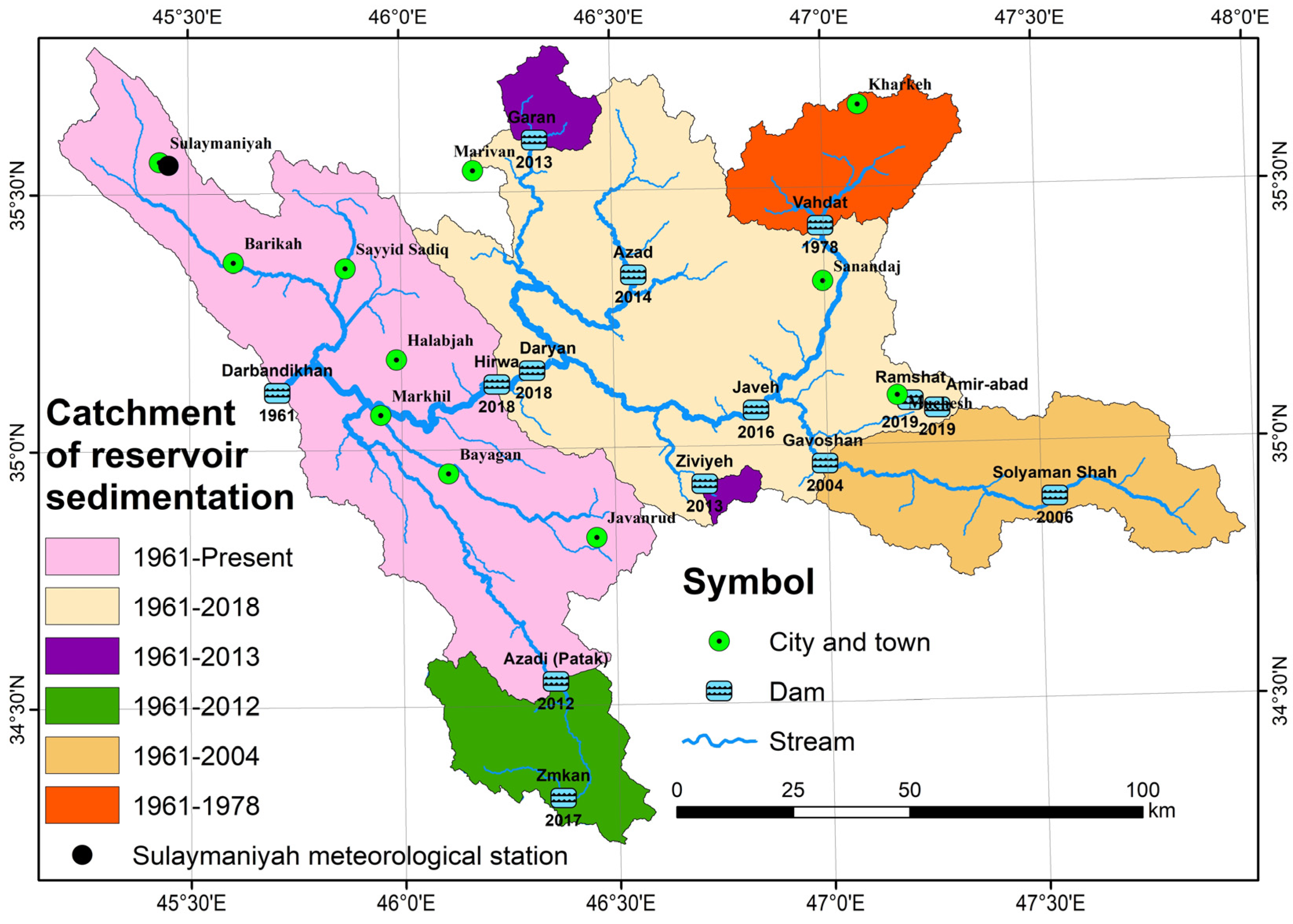
| Period | Area of the Sedimentation Catchment for Darbandikhan Dam (km2) | Area of the Catchment % | Event and the Year | Reference of the Event |
|---|---|---|---|---|
| 1961 | 16,463.1 | 100 | Building Darbandikhan dam | [52] |
| 1978 | 15,403.5 | 93.6 | Building Vahdat dam | [55] |
| 2004 | 13,329.8 | 81.0 | Building Gavoshan dam | [56] |
| 2012 | 12,253.9 | 74.4 | Building Azadi dam | [57] |
| 2013 | 11,865 | 72.1 | Building Garan and Ziviyeh dam | [57] |
| 2018 | 5965.8 | 36.2 | Building Hirwa and Daryan dams | [58] |
| Method | The Article Used within Iran–Iraq–Turkey | Note | Equation |
|---|---|---|---|
| [25] | (3) | ||
| [23] | 340 < PA < 3500 mm | (4) | |
| [34,35,46,48] | F > 55 mm | (5) | |
| [29] | (6) | ||
| [50,83] | (7) | ||
| [47,84,85] | (8) |
| Structure Class (s) | Value | Size | Soil Database |
|---|---|---|---|
| Very fine granular | 1 | 1–2 mm | G (good) |
| Fine granular | 2 | 2–5 mm | N (normal) |
| Medium or coarse granular | 3 | 5–10 mm | P (poor) |
| Blocky, platy, or massive | 4 | N10 mm | H (peaty topsoil) |
| Permeability Class | Value | Texture |
|---|---|---|
| Fast and very fast | 1 | Sand |
| Moderate fast | 2 | Loamy sand, sandy loam |
| Moderate | 3 | Loam, silty loam |
| Moderate low | 4 | Sandy clay loam, clay loam |
| Slow | 5 | Silty clay loam, sand clay |
| Very slow | 6 | Silty clay, clay |
| Name | C Factor | References |
|---|---|---|
| Open Shrublands | 0.10 | [102] |
| Savannas | 0.05 | [102] |
| Grasslands | 0.01 | [102] |
| Permanent Wetlands | 0 | [13] |
| Croplands | 0.3 | [12,13,102] |
| Urban and Built-Up Lands | 0 | [13,102] |
| Cropland/Natural Vegetation Mosaics | 0.3 | [12,13,102] |
| Barren | 0 | [13,102] |
| Water Bodies | 0 | [12,13] |
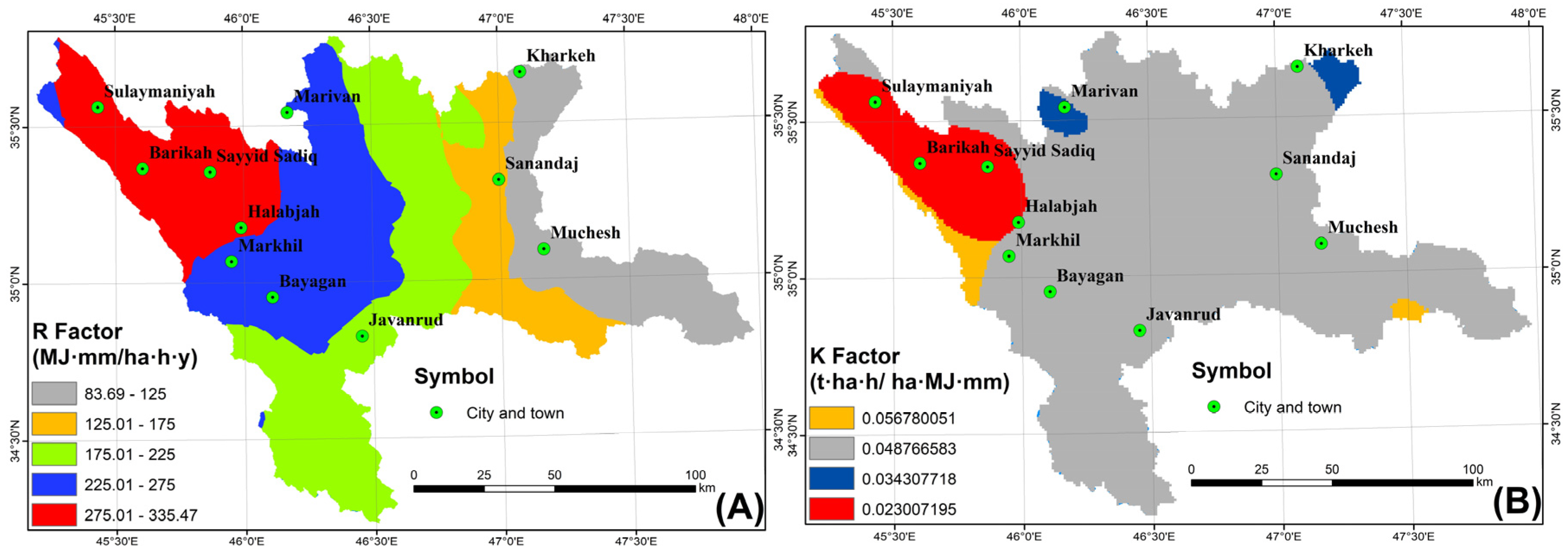
| R Factor | Minimum | Maximum | Mean | SD |
|---|---|---|---|---|
| Equation (3) | 215.80 | 332.54 | 290.14 | 25.44 |
| Equation (4) | 224.71 | 346.92 | 302.53 | 26.64 |
| Equation (5) | 83.69 | 335.47 | 210.40 | 64.18 |
| Equation (6) | 106.75 | 347.05 | 242.71 | 60.30 |
| Equation (7) | 129.04 | 345.63 | 245.28 | 54.81 |
| Equation (8) | 229.95 | 446.79 | 352.64 | 54.39 |
| Soil Type | Texture Class | Sand% | Silt% | Clay% | K Factor |
|---|---|---|---|---|---|
| Lithosols | Loam | 43 | 34 | 23 | 0.048767 |
| Chromic Vertisols | Clay | 16 | 29 | 55 | 0.023007 |
| Haplic Xerosols | Clay loam | 23 | 33 | 44 | 0.056780 |
| Calcic Xerosols | Clay loam | 40 | 37 | 23 | 0.063365 |
| C Factor | Minimum | Maximum | Mean | SD |
|---|---|---|---|---|
| Equation (17) | 0.029 | 1 | 0. 618 | 0. 13 |
| Land cover | 0 | 0.3 | 0.091 | 0.127 |
| Equation (18) | 0.213 | 0.579 | 0. 396 | 0. 034 |
| Model No. | Minimum | Maximum | Mean | SD |
|---|---|---|---|---|
| 1 | 0.125 | 0.128 | 0.126 | 0.0014 |
| 2 | 0.509 | 0.519 | 0.511 | 0.0059 |
| 3 | 0.402 | 0.420 | 0.410 | 0.0074 |
| 4 | 0.172 | 0.176 | 0.174 | 0.0017 |
| IC (Equation (22)) | 0.013 | 0. 147 | 0.0327 | 0.0076 |
| Scenarios | C Factor | R Factor | SDR | RSed (km3) | Error % |
|---|---|---|---|---|---|
| 18 | Equation (18) | Equation (5) | SDR1 | 22.29 | 0.32 |
| 66 | Land cover | Equation (5) | SDR4 | 22.445 | 1.01 |
| 61 | Land cover | Equation (7) | SDR4 | 24.97 | 12.34 |
| 62 | Land cover | Equation (6) | SDR4 | 25.09 | 12.89 |
| 13 | Equation (18) | Equation (7) | SDR1 | 26.50 | 19.24 |
| 14 | Equation (18) | Equation (6) | SDR1 | 26.57 | 19.54 |
Disclaimer/Publisher’s Note: The statements, opinions and data contained in all publications are solely those of the individual author(s) and contributor(s) and not of MDPI and/or the editor(s). MDPI and/or the editor(s) disclaim responsibility for any injury to people or property resulting from any ideas, methods, instructions or products referred to in the content. |
© 2023 by the authors. Licensee MDPI, Basel, Switzerland. This article is an open access article distributed under the terms and conditions of the Creative Commons Attribution (CC BY) license (https://creativecommons.org/licenses/by/4.0/).
Share and Cite
Othman, A.A.; Ali, S.S.; Salar, S.G.; Obaid, A.K.; Al-Kakey, O.; Liesenberg, V. Insights for Estimating and Predicting Reservoir Sedimentation Using the RUSLE-SDR Approach: A Case of Darbandikhan Lake Basin, Iraq–Iran. Remote Sens. 2023, 15, 697. https://0-doi-org.brum.beds.ac.uk/10.3390/rs15030697
Othman AA, Ali SS, Salar SG, Obaid AK, Al-Kakey O, Liesenberg V. Insights for Estimating and Predicting Reservoir Sedimentation Using the RUSLE-SDR Approach: A Case of Darbandikhan Lake Basin, Iraq–Iran. Remote Sensing. 2023; 15(3):697. https://0-doi-org.brum.beds.ac.uk/10.3390/rs15030697
Chicago/Turabian StyleOthman, Arsalan Ahmed, Salahalddin S. Ali, Sarkawt G. Salar, Ahmed K. Obaid, Omeed Al-Kakey, and Veraldo Liesenberg. 2023. "Insights for Estimating and Predicting Reservoir Sedimentation Using the RUSLE-SDR Approach: A Case of Darbandikhan Lake Basin, Iraq–Iran" Remote Sensing 15, no. 3: 697. https://0-doi-org.brum.beds.ac.uk/10.3390/rs15030697