
BiTSRS: A Bi-Decoder Transformer Segmentor for High-Spatial-Resolution Remote Sensing Images


School of Electronics and Information, Northwestern Polytechnical University, Xi’an 710129, China
*
Author to whom correspondence should be addressed.
Remote Sens. 2023, 15(3), 840; https://0-doi-org.brum.beds.ac.uk/10.3390/rs15030840
Submission received: 29 December 2022
/
Revised: 29 January 2023
/
Accepted: 30 January 2023
/
Published: 2 February 2023
(This article belongs to the Special Issue Signal Processing Theory and Methods in Remote Sensing)
Abstract
:Semantic segmentation of high-spatial-resolution (HSR) remote sensing (RS) images has been extensively studied, and most of the existing methods are based on convolutional neural network (CNN) models. However, the CNN is regarded to have less power in global representation modeling. In the past few years, methods using transformer have attracted increasing attention and generate improved results in semantic segmentation of natural images, owing to their powerful ability in global information acquisition. Nevertheless, these transformer-based methods exhibit limited performance in semantic segmentation of RS images, probably because of the lack of comprehensive understanding in the feature decoding process. In this paper, a novel transformer-based model named the bi-decoder transformer segmentor for remote sensing (BiTSRS) is proposed, aiming at alleviating the problem of flexible feature decoding, through a bi-decoder design for semantic segmentation of RS images. In the proposed BiTSRS, the Swin transformer is adopted as encoder to take both global and local representations into consideration, and a unique design module (ITM) is designed to deal with the limitation of input size for Swin transformer. Furthermore, BiTSRS adopts a bi-decoder structure consisting of a Dilated-Uper decoder and a fully deformable convolutional network (FDCN) module embedded with focal loss, with which it is capable of decoding a wide range of features and local detail deformations. Both ablation experiments and comparison experiments were conducted on three representative RS images datasets. The ablation analysis demonstrates the contributions of specifically designed modules in the proposed BiTSRS to performance improvement. The comparison experimental results illustrate that the proposed BiTSRS clearly outperforms some state-of-the-art semantic segmentation methods.
1. Introduction
Semantic segmentation, referring to pixel-level classification in a single image, plays an important role in remote sensing (RS) image processing, with which better understanding of RS images can be acquired for further applications, including resource exploitation, geographical mapping, smart city planning, etc. [1,2,3,4,5,6,7]. Semantic segmentation of RS images has been studied for a long time on low resolution datasets [8,9]. With the development of high-resolution video satellites, studies on semantic segmentation are focusing on RS images with high resolutions and large physical scales [10,11,12,13]. While the resolution of RS images greatly expands the application scenarios of semantic segmentation, it also brings new challenges to the existing methods.
RS semantic segmentation models were initially built according to semantic segmentation methods for natural scenes. After Alexnet won the championship in 2012 [14], models based on convolutional neural networks (CNNs) became mainstream in computer vision (CV) image processing tasks [15,16,17,18,19]. The original CNN-based semantic segmentation methods employed a CNN for feature extraction, and images were divided into small patches. As a result, each pixel was classified according to the information in the individual patches [20,21,22]. Some works also tried to combine hand-crafted structures with a CNN. For example, in [23], the conditional random field (CRF) was embedded in fully connected layers for segmentation. However, these patch-wise approaches could hardly achieve fine pixel classification and were usually not end-to-end pipelines. Long et al. [24] proposed a fully convolutional network (FCN) for semantic segmentation, which was proved to be irreplaceable in pixel-wise classification, with much better performance than the other fully-connected networks. Based on this, Ronneberger et al. [25] constructed the U-Net with an encoder–decoder structure for downsampling and upsampling, which was widely employed in later works. These two works demonstrated the effectiveness of CNN in an encoder–decoder structure for semantic segmentation. Substantial studies with excellent performance have been conducted on this basis, including U-Net++ [26], Deeplabv3+ [27], PSPNet [28], etc.
These CNN-based models designed for natural scenes could also be used in RS image segmentation tasks. However, the direct model migration totally ignored the characteristics of RS images, which were usually characterized by higher resolutions, larger physical scales, smaller objects, and more various class distributions. Consequently, to achieve better performance in semantic segmentation of RS images, extra designs are usually introduced into the above CNN-based models [29,30,31,32,33,34]. Additionally, some works use extra designs for RS, regarding segmentation to detection when small objects are involved, especially for wide-area motion imagery (WAMI) [35,36].
The original CNN-based models are frequently blamed for their lack of ability in global representation modeling. In recent years, a transformer was introduced into a CV field [37] as a substitute for a CNN for its remarkable capability in global representation modeling, with the price of local information loss, hence resulting in precision descending. To settle this problem, attempts have been made to introduce the characteristics of CNNs into transformers [38,39,40,41,42,43]. A Swin transformer [43] employing window multi-head self-attention (W-MSA) and shifted window multi-head self-attention (SW-MSA), both of which are powerful structures for global and local feature extraction, is one of the most excellent solutions. The Swin transformer is such an exceptional work that it has been adopted as the backbone and produced promising experimental results in multi-field studies [44,45,46,47,48,49]. The recently built models for semantic segmentation of RS images generally employed a Swin transformer as the backbone, either focusing on introducing the properties of CNNs into transformers or on rearranging the encoder format to deal with the concrete application scenarios [47,48,50]. Nevertheless, the Swin transformer is designed to have a tiny input scale for convenience (224 × 224 pixels or 384 × 384 pixels) such that a comparatively lower time cost is required in the training process, and when it is applied to RS images, the input images are usually large-scale (512 × 512 pixels or 1024 × 1024 pixels), which may cause global information loss in feature extraction. Moreover, the delicate designs of the decoder are commonly ignored in the existing RS segmentation models built on the Swin transformer.
To address these two issues, in this paper, a novel Swin-transformer-based model named the bi-decoder transformer segmentor for remote sensing (BiTSRS) is proposed. The BiTSRS is based on the Swin transformer and adopts an input transform module (ITM) to deal with the problem of large-scale input images. With the ITM, the Swin transformer is capable of extracting global and local features from small-scale feature maps instead of original RS images, thereby avoiding the loss of global representations. Inspired by UperNet [51] and FCN [24], the proposed BiTSRS employs a bi-decoder structure for hidden feature decoding. The specifically designed bi-decoder structure consists of a Dilated-Uper decoder and an FDCN decoder, which deal with the coarse and fine features in decoding, respectively. Specifically, the Dilated-Uper decoder restores the scale, which is reduced in the downsampling process of the encoder. Meanwhile, the FDCN decoder performs a refinement, adopting deformable convolution for detailed semantic segmentation. With this bi-decoder strategy, BiTSRS is capable of acquiring a wide range of semantic information on RS images and deformable representations in detail. The main contributions of this article can be summarized as follows.
- An improved transformer-based model is proposed that combines the Swin transformer and a bi-decoder structure to perform semantic segmentation of RS images. This new framework is capable of modeling both global and local representations while decoding coarse and fine features.
- For larger-scale RS images, an input transform module (ITM) is proposed to transform the inputs with large spatial scales to the ones with compatible scales for the Swin transformer. The ITM is designed to be a plug-and-play module, which can be easily implanted in the Swin transformer to make it more suitable for RS images.
- A novel bi-decoder structure was specifically designed to decode the features extracted by the Swin transformer encoder. With this bi-decoder structure, BiTSRS can decode the features in a larger receptive field without losing the deformations in detail.
- A more appropriate loss is considered to deal with the problems of complex background samples and class distribution of the segmentation process in the auxiliary FDCN decoder. Such loss is illustrated to be more effective in distinguishing the hard samples by introducing a focusing parameter.
The rest of this article is organized as follows. Section 2 introduces the related works of semantic segmentation of RS images and methods using vision transformers. Then, the overall framework of the proposed BiTSRS is presented in Section 3, each component of which is concretely described. In Section 4, both comparison experiments and ablation studies are applied, and the experimental results are presented and analyzed. Finally, the conclusions are drawn in Section 5.
2. Related Works
2.1. Semantic Segmentation of RS Images with CNNs
Semantic segmentation denotes the pixel-level classification of a single image, namely, labeling the image pixel by pixel according to semantic attributes. The CNN is widely acknowledged because of its powerful ability to acquire deep features of images, and thus it is also applied in semantic segmentation. The CNN-based methods for semantic segmentation have been adequately studied, and numerous excellent works have been proposed, such as FCN [24], U-net [25], and those presented in [26,27,28,52,53,54]. These general semantic segmentation models have been successfully applied in various natural scenes, including automatic driving, medical image processing, etc.
Nevertheless, some unique challenges arise when semantic segmentation is applied to RS images, such as small-scale objects, complex background samples, and serious class variances, which make direct migration of the semantic segmentation models for natural scenes to RS images ineffective. Some works introduce these general CNN-based models into semantic segmentation of RS images by adopting refinement strategies or hand-crafted methods. Du et al. [55] introduced object-based image analysis (OBIA) into RS images, and Mou et al. [56] adopted spatial and channel relation modules to capture the relationships between pixels and channels. Another form of refinement was explored in [57] by Zheng et al., who proposed a foreground-aware relation module to optimize the foreground awareness. More recently, models combined with attention mechanism were widely studied, aiming to impel the networks to focus more on significant foreground objects rather than the complex background [32,33,58,59].
2.2. Semantic Segmentation of RS Images Using Transformer
The transformer is a pure attention architecture first proposed in natural language processing (NLP) [60], aiming to capture more long-range dependencies between tokens. Dosovitskiy et al. explored its feasibility in image processing and proved its effectiveness in acquiring global relations of images [37]. Transformers have been widely applied in downstream tasks, such as image classification [37], object detection [61], and semantic segmentation [62,63,64]. The CNN backbone in FCN is replaced with the vision transformer for segmentation in [62], and progressive upsampling (PUP) strategy was designed in [63] by using a vision transformer backbone. A new multilayer perceptron (MLP) was flexibly developed in [64] for feature mapping based on vision transformer.
Transformers are also utilized for semantic segmentation of RS images as well. For example, Xu et al. [50] proposed a lightweight transformer-based model for efficient segmentation, and Ding et al. [65] introduced a context transformer to embed the contextual information of pixels. Compared with the embedded attention mechanism in CNN models, transformers are fully based on a self-attention mechanism, which is more suitable for global relation capturing in RS images. However, the transformer-based models are more likely to lose the local information, which is also crucial for RS image processing and analysis. The Swin transformer [43] has W-MSA and SW-MSA blocks, in which self-attention is calculated in individual windows and merged with window shifts. With this strategy, Swin transformer is capable of extracting both global and local features, which is a better option for semantic segmentation of RS images. He et al. [47] proposed a Swin-transformer-based model embedded with a U-net structure, Gao et al. [48] fused a Swin transformer and CNN for feature extraction, and Zhang et al. [49] proposed a transformer–CNN hybrid model, for semantic segmentation of RS images. Although promising results have been achieved in these works, more attention is paid to building a powerful encoder by combining CNN with Swin transformer, rather than the delicate design of the decoder. Furthermore, RS images usually have large spatial scales, yet the Swin transformer needs a small-scale input. To handle these problems, a new Swin-transformer-based framework, bi-decoder transformer for RS image semantic segmentation (BiTSRS), is proposed in this paper.
3. Method
In this section, a complete architecture of the proposed BiTSRS is presented, and the concrete details of the novel modules, namely, ITM, Dilated-Uper decoder, and FDCN decoder are described. The adopted focal loss is also explained, which is believed to be more reasonable than the widely used cross-entropy loss.
As shown in Figure 1, the proposed BiTSRS consists of four crucial components: the Input Transform Module (ITM), Swin transformer encoder, Dilated-Uper decoder, and the auxiliary decoder FDCN. The proposed BiTSRS adopts the typical encoder–decoder framework architecture, employing the Swin transformer as the encoder for deep feature extraction and image internal correlation modeling, and two decoders for feature map reconstruction. Specifically, the large-scale RS images are firstly transformed by ITM to obtain appropriate inputs for Swin transformer encoder, and the Swin encoder calculates the attention maps to acquire the global and local representations of the input images. Then, the Dilated-Uper decoder and FDCN decoder are employed to reconstruct the hidden representations of the Swin encoder, expanding the receptive field while preserving the fine deformations of the feature maps.
3.1. Input Transform Module
The Input Transform Module (ITM) is designed to handle the problem of the Swin transformer requiring small-scale inputs, even though RS images are usually large in scale. It has been proved that better results can be achieved by dividing the sampling process into several steps rather than sampling the feature maps directly [63]. Therefore, as depicted in Figure 2, the input size is reduced by downsampling the RS images in the first two steps of ITM. To fully utilize both semantic and appearance information of the input images, ITM extracts features from different scales of RS images, and further aggregates these various scales of feature maps with downsampling and upsampling. Downsampling is performed by the transformer block, which is composed of two groups of a convolutional layer and a batch normalization layer with residual connections, and upsampling is performed by bilinear interpolation. A global average pooling (GAP) branch is also utilized to integrate more scene understandings, while expecting more deep representation to compensate for information loss in the previous scale reduction. It is notable that in the ITM, residual connections and lateral convolutions are employed to enhance the feature transmission and smooth the feature maps progressively.
For a given RS image , it is firstly transformed to feature map with the size of . To utilize semantic information in deep layers, the feature map is downsampled to acquire feature maps with four different scales (, , , and ). A GAP branch is also adopted in ITM to acquire better scene understanding for the entire image. These four feature maps with different scales are finally resized to , the same scale as , and are then concatenated to form the final output serving as the input of Swin transformer encoder.
The output of ITM can be then described as follows:
where in the formula denotes the concatenation operations, denote the four upsampled feature maps, and denotes the output of GAP branch.
Before being fed into the Swin transformer encoder, the feature map is firstly divided into non-overlapping patches by the patch partition module. Each patch is regarded as a "token," and the patch size is set to . The split patches are then projected into embedding features, using a linear projection in the patch embedding module.
3.2. Swin Transformer Encoder
Swin transformer is a widely used transformer architecture for feature extraction that integrates the advantages of both the transformer and convolutional neural networks (CNNs) [43]. To acquire abundant contextual information, the Swin transformer is adopted in the proposed BiTSRS as the encoder after the ITM. Differently from ViT, the Swin transformer combines the window block and shifted window block, enabling the Swin encoder to obtain both global and local information of the input feature map. For a hierarchical multi-scale representation, the Swin encoder merges the patches after each stage. As a result, the scale of feature maps will get a reduction, and the dimensions will be doubled.
As shown in Figure 1, the main component of each Swin transformer stage is the Swin transformer block, including a window block and a shifted window block. The difference between them is that window block employs window multi-head self-attention (W-MSA) and the shifted window block employs shifted window multi-head self-attention (SW-MSA) for attention calculating. Specifically, instead of computing the attention in each individual small patch, Swin transformer blocks use non-overlapped local windows for attention calculation. However, separate W-MSA of fixed windows lacks connections across windows, and thus, SW-MSA is proposed to strengthen the correlations between windows, as illustrated in Figure 3. To balance the capability of image modeling and the computational efficiency, the basic version of the Swin transformer is adopted in BiTSRS, which consists of four stages with 2, 2, 18, and 2 Swin transformer blocks, respectively.
As illustrated in Figure 3b, for a given input vector , which is actually the output of the previous layer, the output can be calculated as follows:
Compared with the traditional attention mechanism, the two successive Swin transformer blocks acquire attention information within individual windows and model the correlations between the windows in a two-step process, which can be described as follows:
where denotes the output of the window block and denotes the output of the shifted window block. In BiTSRS, the numbers of Swin transformer blocks in the four Swin transformer stages are set to be 2, 2, 18, and 2, respectively.
3.3. Dilated-Uper Decoder
The hierarchical feature maps produced by the Swin transformer encoder are sent to the Dilated-Uper decoder for semantic segmentation. Dilated convolution is widely used in semantic segmentation to enlarge the receptive field of the network as compensation for the limited local context of the convolutional neural networks. However, BiTSRS adopts the ITM and the Swin transformer encoder to capture the long-range dependencies between pixels, and the dilated convolution is exploited in the decoder to further enhance the global context. Inspired by UperNet [51], the proposed BiTSRS employs two modules, namely, Pyramid Pooling Module (PPM) [28] and Feature Pyramid Network (FPN) [66], to reconstruct detailed features and on this basis, extra dilated convolution is applied to enlarge the decoding receptive field. Specifically, as illustrated in Figure 4, the topmost feature map of the hierarchical inputs is fed into PPM for pyramid pooling, and the corresponding output is combined with the other three feature maps in the FPN.
The PPM employs a pyramid pooling strategy to acquire global scene understanding, which helps with processing complex background samples. The pooling scales adopted in the PPM are set as 1, 2, 3, and 6, respectively. The pyramid pooling results are resized, concatenated, and convolved to generate a feature map with the same dimension as the input. In the FPN, the feature maps are resized to a higher dimension with a lateral convolution, which is used for feature map smoothing and dimension matching. The three resulting feature maps are combined with the output of PPM for further concatenating and convolution.
In Dilated-Uper decoder, extra convolutions are added before concatenating the outputs of FPN, which are used to construct hierarchical dilated convolutions. Apart from applying the standard convolutions on the top two feature maps, the other two feature maps are convolved with dilated filters with dilation rates of 2 and 4, respectively.
Dilated convolution pads the convolution kernel with zeros to generate a larger receptive field and introduces a parameter r to represent the dilation rate. The formula of 1D dilated convolution can be described as follows:
where is a 1D vector, and are the input and output features, respectively; is the dilation filter with length L; and r denotes the dilation rate. r is set as 1 when standard convolution is used, and represents filling one zero between each of two adjacent elements of convolution kernel.
It is notable that the dilated convolutions are arranged following the hybrid dilated convolution (HDC) principle, which can be interpreted as the fact that using a set of dilated convolutions with certain hybrid dilation rates can entirely cover the input feature maps without any holes and missing edges.
3.4. Fully Deformable Convolutional Network
The FDCN is designed as the auxiliary decoder of BiTSRS, taking input slightly different from the one of Dilated-Uper decoder, which is the upsampled and concatenated output of the Swin encoder. The Dilated-Uper decoder integrates more global context information, and the FDCN is designed to obtain more details of the input features in decoding. Therefore, the FDCN adopts a more flexible convolution operation named deformable convolution [67] to acquire detailed deformation of the hidden representations. Deformable convolution adaptively samples the input features to adjust the receptive field and thus alleviate multi-scale objects and their deformation. Deformable convolution is defined as follows:
where is an element in the output feature map , is the grid of convolution kernel, is the weight of the element in the input feature map , and are the offsets learned by deformable convolution. Specifically, deformable convolution adopts a parallel convolution branch to learn the offset for each element , the kernel of which is applied over the same input feature map and is of the same spatial scale as the current convolution kernel.
Considering the computation cost, in this work, a single-layer deformable convolution is adopted in FDCN to decode the deformation of input features, which can help with better performance by acquiring more detailed deformations. It is notable that the FDCN decoder is only activated in the training process for network optimization and will not take effect in the inference process. Specifically, the Dilated-Uper decoder and FDCN decoder were both activated to acquire global context dependencies and detailed features, respectively, for training and to obtain the final segmentation results; only the Dilated-Uper decoder was used for inference.
To further improve the effectiveness of this refinement branch, a focal loss is employed in the FDCN (as shown in Equation (6)), which is expected to focus on hard samples in segmentation by introducing a focusing parameter . The losses are defined as follows:
where is the prediction probability, y is the corresponding label, is the cross-entropy loss, and is the focal loss. Consequently, the loss function of the entire network can be written as follows:
where denotes the cross-entropy loss employed by the Dilated-Uper decoder, denotes the focal loss employed by the FDCN decoder, and is the balance coefficient of the loss function for the reason that the focal loss is far smaller than the cross-entropy loss.
4. Experiments
4.1. Datasets
The experiments were conducted on three RS datasets, including the ISPRS Vaihingen dataset, the ISPRS Potsdam dataset, and the LoveDA dataset. The two ISPRS datasets are widely used for RS semantic segmentation tasks, and the LoveDA dataset is a newly released dataset which is more challenging. The details are described as follows.
(1) Vaihingen Dataset: The ISPRS Vaihingen and Potsdam datasets [68] are both commonly evaluated benchmarks in the semantic segmentation of RS images. The Vaihingen dataset is a small-scale dataset with 33 true orthophoto (TOP) images which are collected by advanced airborne sensors and usually divided into small images for training and testing. The Vaihingen dataset covers an area of 1.38 km with 6 different classes of objects, including buildings, trees, low vegetation, cars, clutters, and impervious surfaces. The Vaihingen dataset has a ground sampling distance (GSD) of 0.09 m, making it a high-resolution dataset. The scales of the TOP images range from 1887 to 3816 pixels; and each TOP image has infrared (IR), red (R), and green (G) channels to compose the pseudo-color image. In the experiments, 16 images were selected for training and 17 images for testing, following the common practice. For convenient processing, the TOP images were cropped into 512 × 512 pixels with a stride size of 256 pixels.
(2) Potsdam Dataset: Compared with the Vaihingen dataset, the size of Potsdam dataset is slightly larger, having 38 TOP images collected by advanced airborne sensors. The Potsdam dataset covers an area of 3.42 km with the same 6 classes as the Vaihingen dataset and a GSD of 0.05 m. The TOP images of the Potsdam dataset with fixed size of 6000 × 6000 pixels were also cropped into 512 × 512 pixels with a stride size of 256 pixels. Particularly, 24 images were utilized for training, and the remaining 14 images were used for testing, following the previous studies [48,69,70].
(3) LoveDA Dataset: Land-cover Domain Adaptive semantic segmentation (LoveDA) dataset [71] is a recently released remote sensing dataset with high resolution. Unlike the Vaihingen dataset and Potsdam dataset with a comparatively small scale, the LoveDA dataset contains 5987 images collected with spaceborne sensors, covering an area of 536.15 km with 7 classes, including buildings, roads, water, barren, forest, agriculture, and background. The size of each image in the LoveDA dataset is 1024 × 1024 pixels with a GSD of 0.3 m. Following the official dataset split, 2522 images were used for training and 1669 images for testing in this work.
4.2. Evaluation Metrics
To quantitatively measure and compare the performances in semantic segmentation, the mean intersection over union (mIoU) and the mean accuracy (mAcc) were employed as evaluation metrics in this work.
(1) mIoU: The mean intersection over union (mIoU) is one of the most commonly used evaluation metrics for semantic segmentation. With the confusing matrix shown in Table 1, the mIoU can be defined as follows:
where N is the number of classes. The four items, including true positive (TP), false positive (FP), false negative (FN), and true negative (TN), represent the relationships between ground truth and predictions.
(2) mAcc: The mean accuracy (mAcc) is also an effective evaluation metric for semantic segmentation which is similar to the accuracy in classification tasks. With the confusion matrix, the mAcc can be defined as follows:
4.3. Implementation Details
(1) Training Configuration: To provide a consistent input, the input images in the LoveDA dataset are resized into 512 × 512 pixels, which is the same size as images in the ISPRS Vaihingen and Potsdam datasets. Random resizing, clipping and flipping, and photometric distortion and band normalization were employed for data augmentation. The proposed BiTSRS and the compared models were implemented based on the PyTorch framework. The Adaptive momentum estimation with weight decay (AdamW) [72] optimizer was employed for model training, with the learning rate of and the weight decay of 0.01. To guarantee a reasonable number of training iterations, a polynomial learning rate [73] with a linear warm-up was adopted for the first 1500 iterations with a warm-up ratio of , and the maximum number of iterations was set to 16,000 for the entire training process. The polynomial policy in the rest of the iterations can be described as follows:
where denotes the learning rate in time t, is the initial learning rate, T is the total number of iterations, and is the power of adopted polynomial. Furthermore, for a fair comparison, the following experiments did not employ pretrained models, namely, all methods in the experiments were trained from scratch.
(2) Experimental Environment: All the experiments were conducted on a Linux Ubuntu 18.04 LTS server with a single NVIDIA GeForce RTX 3080 GPU with 10,018 MB of memory.
4.4. Ablation Analysis
A simple framework including a Swin transformer encoder and an UperNet-style decoder without any proposed extra designs was employed as the baseline [43]. To illustrate the effectiveness of the proposed model, the following ablation experiments were performed.
(1) Baseline: The baseline model simply combined the Swin transformer with the UperNet in the encoder–decoder structure, in which the Swin transformer encoder was used to extract features of the input images, and the UperNet was utilized to restore the resolution and generate the segmentation results.
(2) Effectiveness of Input Transform Module: The motivation of designing the ITM was to make the size of input images more appropriate for the Swin transformer encoder. With cascaded ITM, the designed framework is capable of performing semantic segmentation on RS images with large spatial scales, conveniently using the pretrained weights of the Swin transformer trained on the ImageNet dataset. The results for the comparison are shown in Table 2. The first group depicts the results of the baseline model, which loads the pretrained weights (denotes as with pr) with or without the ITM. The middle group is the comparison when the baseline model does not load the pretrained weights with or without the ITM. Additionally, the bottom group is the comparison of the baseline model loading the pretrained weights with or without the ITM, when an input with a larger size of 1024 × 1024 pixels is employed (a smaller size input with 512 × 512 pixels was employed in the previous two groups). It can be observed that when the pretrained Swin transformer;s weights are loaded, improvements of 2.12% in mIoU and 0.28% in mAcc can be obtained by employing the ITM. Even without the pretrained weights, improvements of 1.56% in mIoU and 1.21% in mAcc can still be obtained by employing the ITM. Furthermore, when the framework is applied on larger-scale RS images with a size of 1024 × 1024 pixels, improvements of 2.25% in mIoU and 0.73% in mAcc can also be achieved. The experimental results illustrate that the designed ITM can effectively improve the performance of RS image semantic segmentation, especially for large-scale RS images. Even without pretrained weights, the use of ITM still leads to a salient improvement in semantic segmentation performance.
(3) Effectiveness of the Bi-decoder Design: In this part, the baseline with ITM was employed as the fundamental framework, and the performance improvements of the three specific components (Dilated-Uper decoder, FDCN, and focal loss) in the framework are discussed. The experimental results are shown in Table 3. It can be observed that enclosing any one of the three specific designs in the baseline framework can lead to a performance improvement in semantic segmentation. Improvements could also be observed when their arbitrary combinations were employed in the framework. The best performance was achieved by combining all the three designs in the framework: there were improvements of 2.94% in mIoU and 3.25% in mAcc. These improvements can be attributed to their outstanding capabilities in receptive field expansion, image deformation acquisition, and handling the problem of training sample imbalance.
4.5. Comparison with Some State-of-the-Art Methods
To further demonstrate the effectiveness and superiority of the proposed BiTSRS, 12 state-of-the-art algorithms were adopted for the comparison, including 7 algorithms proposed for general scene segmentation, i.e., FCN [24], U-net [25], PSPNet [28], DeepLabv3+ [27], HRNet [11], and SETR [63], BeiT [74]; and 5 algorithms specially designed for RS images, i.e., STransFuse [48], UNetFormer [75], SwinB-CNN [49], and ST-UNet [47]. The baseline mentioned of our proposed BiTSRS is also included in the comparison. It is noted that all the CNN-based methods are highly optimized versions based on the official implementations. For example, dilated convolution in the ResNet50 backbone is employed in CNN-based methods, such as FCN, U-net, and PSPNet, for better performance.
Particularly, training settings are inconsistent among the RS-specific methods; for example, the cropped size of the image is 1024 × 1024 in UNetFormer [75], 256 × 256 in ST-UNet [47], and 300 × 300 in SwinB-CNN [49]. In addition, test-time augmentation (TTA) strategies are used in UNetFormer [75] and not in other methods. Furthermore, the number of epochs is also different among the methods; for example, there are 100 epochs in ST-UNet [47], 50 epochs in UNetFormer [75], and 16,000 iterations in SwinB-CNN [49]. To make a fair comparison, the RS-specific methods, including UNetFormer, SwinB-CNN, and ST-UNet, were re-trained and re-evaluated under the same experimental settings, including without pretrained weights and testing augmentation, with the same cropped size of the image and number of epochs, etc. As STransFuse [48] does not provide the source code temporarily, its results were directly taken from its paper, since our experimental settings were as same as those in [48].
Three commonly used RS image datasets were used in the comparison experiments, including the ISPRS Vaihingen dataset, the ISPRS Potsdam dataset, and the LoveDA dataset. The comparison results on Vaihingen dataset are listed in Table 4. It can be observed that the proposed BiTSRS achieved the highest mAcc and mIoU on the Vaihingen dataset. From the perspective of the IoU of each class, the proposed BiTSRS achieves an obviously higher IoU for the clutter class, and a comparable IoU for the other five classes to those of the other methods. This is also confirmed by the visualization results depicted in Figure 5. The proposed BiTSRS can effectively segment the clutter class, which is actually the most challenging class in the Vaihingen dataset, and this can be confirmed by the last rows of the visualization images.
The comparison results for the Potsdam dataset are shown in Table 5. The highest mIoU and mAcc were both achieved by the proposed BiTSRS. It can be observed that BiTSRS outperforms the other methods for all classes except the tree class and building class. Similarly to its performance on the Vaihingen dataset, BiTSRS can segment the clutter class more accurately than the other methods, which is consistent with visualization results in Figure 6. With a larger scale than the Vaihingen dataset, the Potsdam dataset has more sufficient data for training, so that better performance is achieved than for the Vaihingen dataset.
Differently from the Vaihingen and Potsdam datasets, semantic segmentation on LoveDA dataset is far more challenging, because of its more complex background samples, inconsistent class distributions, and multi-scale objects. The comparison results on the LoveDA dataset are shown in Table 6, and it can be seen that the proposed BiTSRS still clearly outperforms the other methods by producing the best mIoU and mAcc. Particularly, for the most challenging class in LoveDA dataset, the barren class, the proposed BiTSRS achieves the highest IoU, which can be also observed in Figure 7.
It is also worth noting that the simple FCN method can achieve better results for almost all classes on the Vaihingen dataset, though it has the lowest mIoU for the clutter class. However, for large and complex datasets, i.e., the Potsdam dataset and LoveDA dataset, the FCN performs comparably or even worse than the other methods, indicating that its architecture is not robust for generalization. However, the highly developed CNN-based methods, such as Deeplabv3+ and HRNet, in contrast, are more robust, producing promising results on the three datasets. The general transformer-based methods, such as SETR and BeiT, cannot achieve promising results on all the three datasets, which may be mainly because the unique characteristic of RS images are not specifically considered when designing these networks. The RS-specific transformer-based methods, such as UNetFormer, SwinB-CNN, and ST-UNet, can achieve better performances than other algorithms when they are re-trained and re-evaluated under the same experimental settings as the proposed BiTSRS. For example, the UNetFormer can produce promising results even though it is a real-time method with the smallest model size. Particularly, the Swin-transformer-based methods are more competitive for RS image semantic segmentation; e.g., ST-UNet achieves the best performance among all the compared algorithms. This is mainly because the Swin-transformer structure can better acquire the semantic information in RS images. However, even for the best transformer-based algorithm, i.e., ST-UNet, it is inferior to the proposed BiTSRS.
In summary, the proposed BiTSRS clearly outperforms the compared state-of-the-art methods on all the three datasets, which demonstrates its effectiveness. Specifically, the three delicately designed modules of BiTSRS (ITM, Dilated-Uper decoder, and FDCN) make effective contributions to performance improvement in RS image semantic segmentation. Furthermore, the outstanding capability of BiTSRS in challenging class segmentation illustrates the superiority of the proposed bi-decoder structure, which makes BiTSRS more robust to the challenging and complex samples by acquiring a wide range of receptive fields and more detailed features.
5. Conclusions
In this work, a novel transformer-based semantic segmentation method for RS images, named BiTSRS, was proposed to address the challenges in RS image semantic segmentation. In the proposed BiTSRS, the RS images with large spatial scales are flexibly transformed to appropriate scales with ITM, and then both global and local features of the images are extracted by the Swin transformer encoder. Furthermore, a bi-decoder structure, including a Dilated-Uper decoder and FDCN embedded with focal loss, was designed to acquire both a wide range of receptive fields and detailed deformations for the segmentation task, and to generate the final segmentation prediction. The experimental results on three challenging RS datasets demonstrated the effectiveness and advancement of the proposed BiTSRS in semantic segmentation of RS images, especially for segmentation of hard classes that are easily confused. With the ablation analysis, each component of BiTSRS was discussed in detail to illustrate its contribution to the overall performance improvement. The strategies designed in this work provide insights for future research, and further improvements can be expected by exploring more advanced transformer-based models and more effective loss functions.
Author Contributions
Y.L. and Y.W. conceived of the idea; Y.L. verified the idea and designed the study; Y.L. and Y.Z. analyzed the experimental results; Y.L. and Y.Z. wrote the paper; Y.Z., S.M. and Y.W. gave comments on and suggestions for the manuscript. All authors have read and agreed to the published version of the manuscript.
Funding
This work was supported in part by the National Natural Science Foundation of China under Grant 62171381 and in part by the Fundamental Research Funds for the Central Universities.
Data Availability Statement
The Potsdam and Vaihingen datasets were published by the International Society for Photogrammetry and Remote Sensing (ISPRS) and can be accessed at https://www.isprs.org/education/benchmarks/UrbanSemLab/default.aspx, accessed on 27 December 2022. The LoveDA dataset is available at https://github.com/Junjue-Wang/LoveDA, accessed on 27 December 2022.
Conflicts of Interest
The authors declare no conflict of interest.
References
- Liu, Y.; Ren, Q.; Geng, J.; Ding, M.; Li, J. Efficient Patch-Wise Semantic Segmentation for Large-Scale Remote Sensing Images. Sensors 2018, 18, 3232. [Google Scholar] [CrossRef]
- Kampffmeyer, M.; Salberg, A.B.; Jenssen, R. Semantic segmentation of small objects and modeling of uncertainty in urban remote sensing images using deep convolutional neural networks. In Proceedings of the IEEE Conference on Computer Vision and Pattern Recognition Workshops, Las Vegas, NV, USA, 26 June–1 July 2016; pp. 1–9. [Google Scholar] [CrossRef]
- Luo, H.; Chen, C.; Fang, L.; Khoshelham, K.; Shen, G. Ms-rrfsegnet: Multiscale regional relation feature segmentation network for semantic segmentation of urban scene point clouds. IEEE Trans. Geosci. Remote Sens. 2020, 58, 8301–8315. [Google Scholar] [CrossRef]
- Khan, S.A.; Shi, Y.; Shahzad, M.; Zhu, X.X. FGCN: Deep Feature-based Graph Convolutional Network for Semantic Segmentation of Urban 3D Point Clouds. In Proceedings of the IEEE/CVF Conference on Computer Vision and Pattern Recognition Workshops (CVPRW), Seattle, WA, USA, 14–19 June 2020. [Google Scholar] [CrossRef]
- Zhao, J.; Zhou, Y.; Shi, B.; Yang, J.; Zhang, D.; Yao, R. Multi-stage fusion and multi-source attention network for multi-modal remote sensing image segmentation. ACM Trans. Intell. Syst. Technol. TIST 2021, 12, 1–20. [Google Scholar] [CrossRef]
- Bi, H.; Xu, L.; Cao, X.; Xue, Y.; Xu, Z. Polarimetric SAR image semantic segmentation with 3D discrete wavelet transform and Markov random field. IEEE Trans. Image Process. 2020, 29, 6601–6614. [Google Scholar] [CrossRef]
- Yin, G.; Verger, A.; Descals, A.; Filella, I.; Peñuelas, J. A broadband green-red vegetation index for monitoring gross primary production phenology. J. Remote Sens. 2022, 2022, 9764982. [Google Scholar] [CrossRef]
- Alemohammad, H.; Booth, K. LandCoverNet: A global benchmark land cover classification training dataset. arXiv 2020, arXiv:2012.03111. [Google Scholar]
- Tong, X.Y.; Xia, G.S.; Lu, Q.; Shen, H.; Li, S.; You, S.; Zhang, L. Land-cover classification with high-resolution remote sensing images using transferable deep models. Remote Sens. Environ. 2020, 237, 111322. [Google Scholar] [CrossRef]
- Chen, L.; Letu, H.; Fan, M.; Shang, H.; Tao, J.; Wu, L.; Zhang, Y.; Yu, C.; Gu, J.; Zhang, N.; et al. An Introduction to the Chinese High-Resolution Earth Observation System: Gaofen-1˜ 7 Civilian Satellites. J. Remote Sens. 2022, 2022, 9769536. [Google Scholar] [CrossRef]
- Wang, J.; Sun, K.; Cheng, T.; Jiang, B.; Deng, C.; Zhao, Y.; Liu, D.; Mu, Y.; Tan, M.; Wang, X.; et al. Deep high-resolution representation learning for visual recognition. IEEE Trans. Pattern Anal. Mach. Intell. 2020, 3, 3349–3364. [Google Scholar] [CrossRef] [Green Version]
- Jiang, S.; Jiang, C.; Jiang, W. Efficient structure from motion for large-scale UAV images: A review and a comparison of SfM tools. ISPRS J. Photogramm. Remote Sens. 2020, 167, 230–251. [Google Scholar] [CrossRef]
- Hoeser, T.; Kuenzer, C. Object detection and image segmentation with deep learning on earth observation data: A review-part i: Evolution and recent trends. Remote Sens. 2020, 12, 1667. [Google Scholar] [CrossRef]
- Krizhevsky, A.; Sutskever, I.; Hinton, G.E. Imagenet classification with deep convolutional neural networks. Commun. ACM 2012, 60, 84–90. [Google Scholar] [CrossRef]
- Ma, M.; Mei, S.; Wan, S.; Wang, Z.; Hua, X.S.; Feng, D.D. Graph Convolutional Dictionary Selection With L2,p Norm for Video Summarization. IEEE Trans. Image Process. 2022, 31, 1789–1804. [Google Scholar] [CrossRef]
- Liu, H.; Li, W.; Xia, X.G.; Zhang, M.; Gao, C.Z.; Tao, R. Central attention network for hyperspectral imagery classification. IEEE Trans. Neural Netw. Learn. Syst. 2022. [Google Scholar] [CrossRef]
- Zhang, Y.; Li, W.; Zhang, M.; Wang, S.; Tao, R.; Du, Q. Graph Information Aggregation Cross-Domain Few-Shot Learning for Hyperspectral Image Classification. IEEE Trans. Neural Netw. Learn. Syst. 2022. [Google Scholar] [CrossRef]
- Li, W.; Gao, Y.; Zhang, M.; Tao, R.; Du, Q. Asymmetric feature fusion network for hyperspectral and SAR image classification. IEEE Trans. Neural Netw. Learn. Syst. 2022. [Google Scholar] [CrossRef]
- Ren, S.; He, K.; Girshick, R.; Sun, J. Faster r-cnn: Towards real-time object detection with region proposal networks. In Proceedings of the Advances in Neural Information Processing Systems, Montreal, QC, Canada, 7–12 December 2015; Volume 28. [Google Scholar]
- Ciresan, D.; Giusti, A.; Gambardella, L.; Schmidhuber, J. Deep neural networks segment neuronal membranes in electron microscopy images. In Proceedings of the Advances in Neural Information Processing Systems, Montreal, QC, Canada, 7–12 December 2015; Volume 25. [Google Scholar]
- Farabet, C.; Couprie, C.; Najman, L.; LeCun, Y. Learning Hierarchical Features for Scene Labeling. IEEE Trans. Pattern Anal. Mach. Intell. 2013, 35, 1915–1929. [Google Scholar] [CrossRef]
- Ganin, Y.; Lempitsky, V.S. N4-Fields: Neural Network Nearest Neighbor Fields for Image Transforms. In Proceedings of the 12th Asian Conference on Computer Vision, Singapore, 1–5 November 2014. [Google Scholar]
- Chen, L.C.; Papandreou, G.; Kokkinos, I.; Murphy, K.; Yuille, A.L. Semantic image segmentation with deep convolutional nets and fully connected crfs. arXiv 2014, arXiv:1412.7062. [Google Scholar]
- Long, J.; Shelhamer, E.; Darrell, T. Fully convolutional networks for semantic segmentation. In Proceedings of the IEEE Conference on Computer Vision and Pattern Recognition, Boston, MA, USA, 7–12 June 2015; pp. 3431–3440. [Google Scholar]
- Ronneberger, O.; Fischer, P.; Brox, T. U-net: Convolutional networks for biomedical image segmentation. In Proceedings of the International Conference on Medical Image Computing and Computer-Assisted Intervention, Munich, Germany, 5–9 October 2015; pp. 234–241. [Google Scholar] [CrossRef]
- Zhou, Z.; Siddiquee, M.M.R.; Tajbakhsh, N.; Liang, J. Unet++: A nested u-net architecture for medical image segmentation. In Deep Learning in Medical Image Analysis and Multimodal Learning for Clinical Decision Support; Springer: Berlin/Heidelberg, Germany, 2018; pp. 3–11. [Google Scholar] [CrossRef] [Green Version]
- Chen, L.C.; Zhu, Y.; Papandreou, G.; Schroff, F.; Adam, H. Encoder-decoder with atrous separable convolution for semantic image segmentation. In Proceedings of the European conference on Computer Vision (ECCV), Munich, Germany, 8–14 September 2018; pp. 801–818. [Google Scholar]
- Zhao, H.; Shi, J.; Qi, X.; Wang, X.; Jia, J. Pyramid Scene Parsing Network. In Proceedings of the Computer Vision and Pattern Recognition, Honolulu, HI, USA, 21–26 July 2017. [Google Scholar]
- Chen, G.; Zhang, X.; Wang, Q.; Dai, F.; Gong, Y.; Zhu, K. Symmetrical dense-shortcut deep fully convolutional networks for semantic segmentation of very-high-resolution remote sensing images. IEEE J. Sel. Top. Appl. Earth Obs. Remote Sens. 2018, 11, 1633–1644. [Google Scholar] [CrossRef]
- Sun, W.; Wang, R. Fully convolutional networks for semantic segmentation of very high resolution remotely sensed images combined with DSM. IEEE Geosci. Remote Sens. Lett. 2018, 15, 474–478. [Google Scholar] [CrossRef]
- Wu, Z.; Gao, Y.; Li, L.; Xue, J.; Li, Y. Semantic segmentation of high-resolution remote sensing images using fully convolutional network with adaptive threshold. Connect. Sci. 2019, 31, 169–184. [Google Scholar] [CrossRef]
- Liu, Y.; Zhu, Q.; Cao, F.; Chen, J.; Lu, G. High-resolution remote sensing image segmentation framework based on attention mechanism and adaptive weighting. ISPRS Int. J. Geo Inf. 2021, 10, 241. [Google Scholar] [CrossRef]
- Li, H.; Qiu, K.; Chen, L.; Mei, X.; Hong, L.; Tao, C. SCAttNet: Semantic Segmentation Network With Spatial and Channel Attention Mechanism for High-Resolution Remote Sensing Images. IEEE Geosci. Remote Sens. Lett. 2021, 18, 905–909. [Google Scholar] [CrossRef]
- Luo, Y.; Han, J.; Liu, Z.; Wang, M.; Xia, G.S. An Elliptic Centerness for Object Instance Segmentation in Aerial Images. J. Remote Sens. 2022, 2022, 9809505. [Google Scholar] [CrossRef]
- Negin, F.; Tabejamaat, M.; Fraisse, R.; Bremond, F. Transforming Temporal Embeddings to Keypoint Heatmaps for Detection of Tiny Vehicles in Wide Area Motion Imagery (WAMI) Sequences. In Proceedings of the 2022 IEEE/CVF Conference on Computer Vision and Pattern Recognition Workshops (CVPRW), New Orleans, LA, USA, 19–20 June 2022; pp. 1431–1440. [Google Scholar] [CrossRef]
- Motorcu, H.; Ates, H.F.; Ugurdag, H.F.; Gunturk, B.K. HM-Net: A Regression Network for Object Center Detection and Tracking on Wide Area Motion Imagery. IEEE Access 2022, 10, 1346–1359. [Google Scholar] [CrossRef]
- Dosovitskiy, A.; Beyer, L.; Kolesnikov, A.; Weissenborn, D.; Zhai, X.; Unterthiner, T.; Dehghani, M.; Minderer, M.; Heigold, G.; Gelly, S.; et al. An image is worth 16x16 words: Transformers for image recognition at scale. arXiv 2020, arXiv:2010.11929. [Google Scholar]
- Wang, W.; Xie, E.; Li, X.; Fan, D.P.; Song, K.; Liang, D.; Lu, T.; Luo, P.; Shao, L. Pyramid vision transformer: A versatile backbone for dense prediction without convolutions. In Proceedings of the IEEE/CVF International Conference on Computer Vision, Montreal, BC, Canada, 11–17 October 2021; pp. 568–578. [Google Scholar] [CrossRef]
- Wang, W.; Xie, E.; Li, X.; Fan, D.P.; Song, K.; Liang, D.; Lu, T.; Luo, P.; Shao, L. Pvt v2: Improved baselines with pyramid vision transformer. Comput. Vis. Media 2022, 8, 415–424. [Google Scholar] [CrossRef]
- Han, K.; Xiao, A.; Wu, E.; Guo, J.; XU, C.; Wang, Y. Transformer in Transformer. Adv. Neural Inf. Process. Syst. 2021, 34, 15908–15919. [Google Scholar]
- Wu, H.; Xiao, B.; Codella, N.; Liu, M.; Dai, X.; Yuan, L.; Zhang, L. CvT: Introducing Convolutions to Vision Transformers. In Proceedings of the IEEE/CVF International Conference on Computer Vision, Montreal, BC, Canada, 11–17 October 2021. [Google Scholar] [CrossRef]
- Mei, S.; Song, C.; Ma, M.; Xu, F. Hyperspectral Image Classification Using Group-Aware Hierarchical Transformer. IEEE Trans. Geosci. Remote Sens. 2022, 60, 1–4. [Google Scholar] [CrossRef]
- Liu, Z.; Lin, Y.; Cao, Y.; Hu, H.; Wei, Y.; Zhang, Z.; Lin, S.; Guo, B. Swin transformer: Hierarchical vision transformer using shifted windows. In Proceedings of the IEEE/CVF International Conference on Computer Vision, Montreal, BC, Canada, 11–17 October 2021; pp. 10012–10022. [Google Scholar]
- Liu, Z.; Ning, J.; Cao, Y.; Wei, Y.; Zhang, Z.; Lin, S.; Hu, H. Video Swin Transformer. In Proceedings of the IEEE/CVF Conference on Computer Vision and Pattern Recognition, New Orleans, LA, USA, 18–24 June 2022. [Google Scholar]
- Liang, J.; Cao, J.; Sun, G.; Zhang, K.; Gool, L.V.; Timofte, R. SwinIR: Image Restoration Using Swin Transformer. In Proceedings of the IEEE/CVF International Conference on Computer Vision, Montreal, BC, Canada, 11–17 October 2021. [Google Scholar] [CrossRef]
- Xu, X.; Feng, Z.; Cao, C.; Li, M.; Wu, J.; Wu, Z.; Shang, Y.; Ye, S. An Improved Swin Transformer-Based Model for Remote Sensing Object Detection and Instance Segmentation. Remote Sens. 2021, 13, 4779. [Google Scholar] [CrossRef]
- He, X.; Zhou, Y.; Zhao, J.; Zhang, D.; Yao, R.; Xue, Y. Swin Transformer Embedding UNet for Remote Sensing Image Semantic Segmentation. IEEE Trans. Geosci. Remote Sens. 2022, 60, 1–15. [Google Scholar] [CrossRef]
- Gao, L.; Liu, H.; Yang, M.; Chen, L.; Wan, Y.; Xiao, Z.; Qian, Y. STransFuse: Fusing Swin Transformer and Convolutional Neural Network for Remote Sensing Image Semantic Segmentation. IEEE J. Sel. Top. Appl. Earth Obs. Remote Sens. 2021, 14, 10990–11003. [Google Scholar] [CrossRef]
- Zhang, C.; Jiang, W.S.; Zhang, Y.; Wang, W.; Zhao, Q.; Wang, C.J. Transformer and CNN Hybrid Deep Neural Network for Semantic Segmentation of Very-high-resolution Remote Sensing Imagery. IEEE Trans. Geosci. Remote Sens. 2022, 60, 1–20. [Google Scholar] [CrossRef]
- Xu, Z.; Zhang, W.; Zhang, T.; Yang, Z.; Li, J. Efficient transformer for remote sensing image segmentation. Remote Sens. 2021, 13, 3585. [Google Scholar] [CrossRef]
- Xiao, T.; Liu, Y.; Zhou, B.; Jiang, Y.; Sun, J. Unified Perceptual Parsing for Scene Understanding. In Proceedings of the European Conference on Computer Vision, Munich, Germany, 8–14 September 2018. [Google Scholar] [CrossRef]
- Badrinarayanan, V.; Kendall, A.; Cipolla, R. Segnet: A deep convolutional encoder-decoder architecture for image segmentation. IEEE Trans. Pattern Anal. Mach. Intell. 2017, 39, 2481–2495. [Google Scholar] [CrossRef]
- Chen, L.C.; Papandreou, G.; Kokkinos, I.; Murphy, K.; Yuille, A.L. Deeplab: Semantic image segmentation with deep convolutional nets, atrous convolution, and fully connected crfs. IEEE Trans. Pattern Anal. Mach. Intell. 2017, 40, 834–848. [Google Scholar] [CrossRef]
- Chen, L.C.; Papandreou, G.; Schroff, F.; Adam, H. Rethinking atrous convolution for semantic image segmentation. arXiv 2017, arXiv:1706.05587. [Google Scholar]
- Du, S.; Du, S.; Liu, B.; Zhang, X. Incorporating DeepLabv3+ and object-based image analysis for semantic segmentation of very high resolution remote sensing images. Int. J. Digit. Earth 2021, 14, 357–378. [Google Scholar] [CrossRef]
- Mou, L.; Hua, Y.; Zhu, X.X. A Relation-Augmented Fully Convolutional Network for Semantic Segmentation in Aerial Scenes. In Proceedings of the 2019 IEEE/CVF Conference on Computer Vision and Pattern Recognition (CVPR), Long Beach, CA, USA, 15–20 June 2019; pp. 12408–12417. [Google Scholar] [CrossRef]
- Zheng, Z.; Zhong, Y.; Wang, J.; Ma, A. Foreground-Aware Relation Network for Geospatial Object Segmentation in High Spatial Resolution Remote Sensing Imagery. In Proceedings of the IEEE/CVF Conference on Computer Vision and Pattern Recognition 2020, Seattle, WA, USA, 13–19 June 2020. [Google Scholar] [CrossRef]
- Ding, L.; Tang, H.; Bruzzone, L. LANet: Local Attention Embedding to Improve the Semantic Segmentation of Remote Sensing Images. IEEE Trans. Geosci. Remote Sens. 2021, 59, 426–435. [Google Scholar] [CrossRef]
- Li, R.; Zheng, S.; Duan, C.; Zhang, C.; Su, J.; Atkinson, P.M. Multi-Attention-Network for Semantic Segmentation of Fine Resolution Remote Sensing Images. IEEE Trans. Geosci. Remote Sens. 2020, 60, 1–3. [Google Scholar] [CrossRef]
- Vaswani, A.; Shazeer, N.; Parmar, N.; Uszkoreit, J.; Jones, L.; Gomez, A.N.; Kaiser, L.; Polosukhin, I. Attention is All you Need. In Proceedings of the Advances in Neural Information Processing Systems 30 (NIPS 2017), Long Beach, CA, USA, 4–9 December 2017. [Google Scholar]
- Carion, N.; Massa, F.; Synnaeve, G.; Usunier, N.; Kirillov, A.; Zagoruyko, S. End-to-End Object Detection with Transformers. In Proceedings of the Computer Vision–ECCV 2020: 16th European Conference, Glasgow, UK, 23–28 August 2020. [Google Scholar]
- Strudel, R.; Garcia, R.; Laptev, I.; Schmid, C. Segmenter: Transformer for Semantic Segmentation. In Proceedings of the IEEE/CVF International Conference on Computer Vision, Montreal, BC, Canada, 11–17 October 2021. [Google Scholar]
- Zheng, S.; Lu, J.; Zhao, H.; Zhu, X.; Luo, Z.; Wang, Y.; Fu, Y.; Feng, J.; Xiang, T.; Torr, P.H.S.; et al. Rethinking Semantic Segmentation from a Sequence-to-Sequence Perspective with Transformers. In Proceedings of the IEEE/CVF Conference on Computer Vision and Pattern Recognition, Nashville, TN, USA, 20–25 June 2021. [Google Scholar]
- Xie, E.; Wang, W.; Yu, Z.; Anandkumar, A.; Alvarez, J.M.; Luo, P. SegFormer: Simple and Efficient Design for Semantic Segmentation with Transformers. Adv. Neural Inf. Process. Syst. 2021, 34, 12077–12090. [Google Scholar]
- Ding, L.; Lin, D.; Lin, S.; Zhang, J.; Cui, X.; Wang, Y.; Tang, H.; Bruzzone, L. Looking Outside the Window: Wider-Context Transformer for the Semantic Segmentation of High-Resolution Remote Sensing Images. arXiv 2021, arXiv:2106.15754. [Google Scholar] [CrossRef]
- Lin, T.Y.; Dollár, P.; Girshick, R.; He, K.; Hariharan, B.; Belongie, S. Feature Pyramid Networks for Object Detection. In Proceedings of the IEEE Conference on Computer Vision and Pattern Recognition, Las Vegas, NV, USA, 27–30 June 2016. [Google Scholar]
- Dai, J.; Qi, H.; Xiong, Y.; Li, Y.; Zhang, G.; Hu, H.; Wei, Y. Deformable Convolutional Networks. In Proceedings of the IEEE International Conference on Computer Vision, Venice, Italy, 22–29 October 2017. [Google Scholar]
- ISPRS, Semantic Labeling Contest (2018). Available online: https://www.isprs.org/education/benchmarks/UrbanSemLab/default.aspx (accessed on 27 December 2022).
- Maggiori, E.; Tarabalka, Y.; Charpiat, G.; Alliez, P. High-resolution aerial image labeling with convolutional neural networks. IEEE Trans. Geosci. Remote Sens. 2017, 55, 7092–7103. [Google Scholar] [CrossRef]
- Mou, L.; Hua, Y.; Zhu, X.X. Relation matters: Relational context-aware fully convolutional network for semantic segmentation of high-resolution aerial images. IEEE Trans. Geosci. Remote Sens. 2020, 58, 7557–7569. [Google Scholar] [CrossRef]
- Wang, J.; Zheng, Z.; Ma, A.; Lu, X.; Zhong, Y. LoveDA: A Remote Sensing Land-Cover Dataset for Domain Adaptive Semantic Segmentation. arXiv 2021, arXiv:2110.08733. [Google Scholar]
- Loshchilov, I.; Hutter, F. Decoupled weight decay regularization. arXiv 2017, arXiv:1711.05101. [Google Scholar]
- Mishra, P.; Sarawadekar, K. Polynomial learning rate policy with warm restart for deep neural network. In Proceedings of the TENCON 2019-2019 IEEE Region 10 Conference (TENCON), Kerala, India, 17–20 October 2019; pp. 2087–2092. [Google Scholar]
- Bao, H.; Dong, L.; Wei, F. BEiT: BERT Pre-Training of Image Transformers. arXiv 2021, arXiv:2106.0825. [Google Scholar]
- Wang, L.; Li, R.; Zhang, C.; Fang, S.; Duan, C.; Meng, X.; Atkinson, P.M. UNetFormer: An UNet-like Transformer for Efficient Semantic Segmentation of Remote Sensing Urban Scene Imagery. ISPRS J. Photogramm. Remote Sens. 2021, 190, 196–214. [Google Scholar] [CrossRef]
Figure 1.
The overall architecture of the proposed BiTSRS. The architecture includes three main parts: an Input Transform Module (ITM) to transform large-scale inputs into small-scale feature maps, a Swin transformer encoder to acquire global and local representations, and a bi-decoder structure to decode coarse and fine information.

Figure 2.
The structure of ITM. The transform blocks with residual connections and the global average pooling (GAP) are used to preserve the original information.
Figure 2.
The structure of ITM. The transform blocks with residual connections and the global average pooling (GAP) are used to preserve the original information.

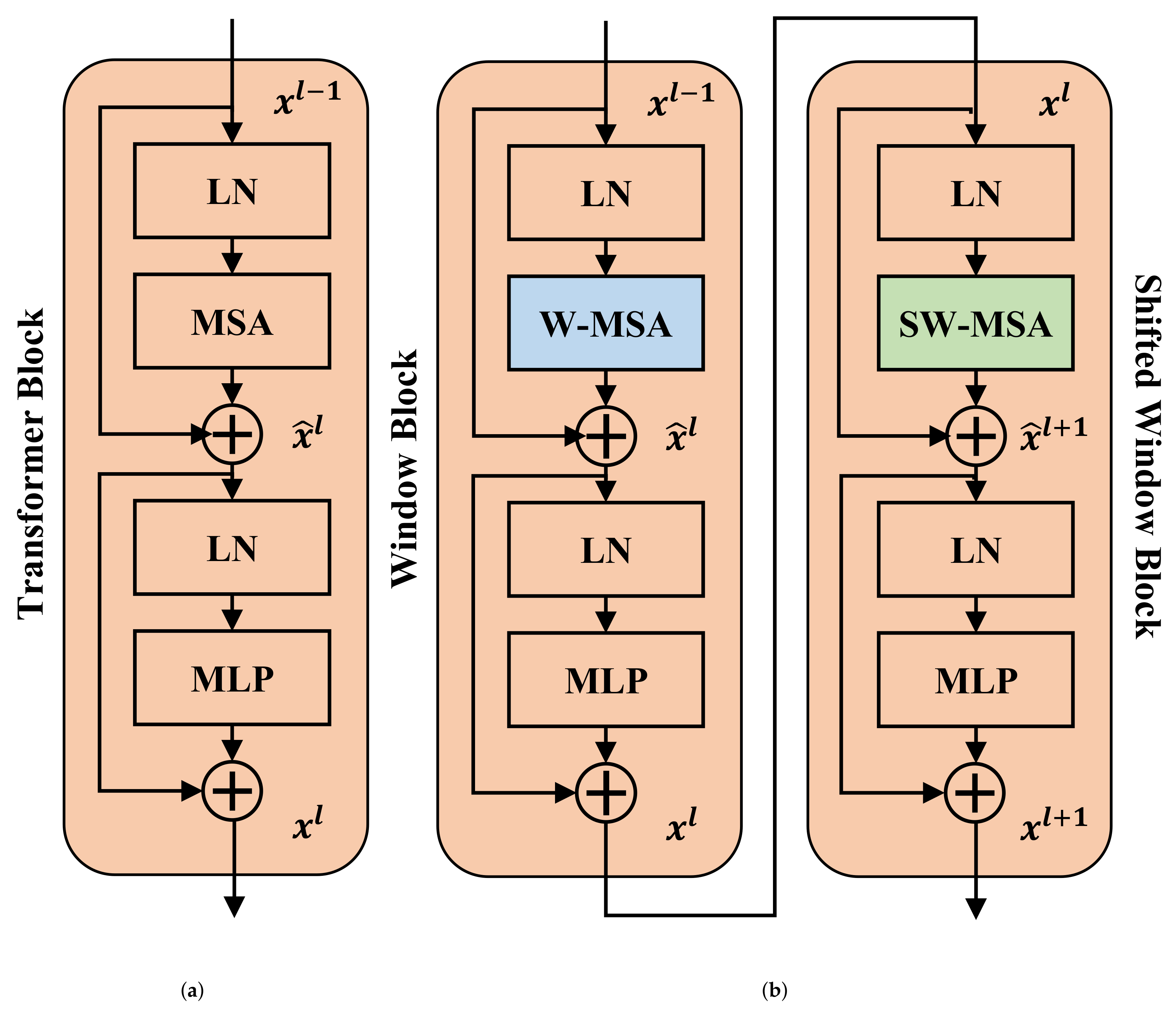
Figure 3.
Illustration of different transformer blocks. (a) The standard transformer block. (b) Two successive Swin transformer blocks, the window block and shifted window block, which compute window multi-head self-attention (W-MSA) and shifted window multi-head self-attention (SW-MSA), respectively. LN and MLP denote layer normalization and multi-layer perceptron, respectively.

Figure 4.
The structure of Dilated-Uper decoder.

Figure 5.
Comparison of visualization results on the ISPRS Vaihingen dataset. (a) FCN. (b) DeepLabv3+. (c) SETR. (d) HRNet. (e) UNetFormer. (f) ST-UNet. (g) Baseline. (h) BiTSRS.
Figure 5.
Comparison of visualization results on the ISPRS Vaihingen dataset. (a) FCN. (b) DeepLabv3+. (c) SETR. (d) HRNet. (e) UNetFormer. (f) ST-UNet. (g) Baseline. (h) BiTSRS.

Figure 6.
Comparison of visualization results on the ISPRS Potsdam dataset. (a) FCN. (b) DeepLabv3+. (c)SETR. (d) HRNet. (e) UNetFormer. (f) ST-UNet. (g) Baseline. (h) BiTSRS.
Figure 6.
Comparison of visualization results on the ISPRS Potsdam dataset. (a) FCN. (b) DeepLabv3+. (c)SETR. (d) HRNet. (e) UNetFormer. (f) ST-UNet. (g) Baseline. (h) BiTSRS.

Figure 7.
Comparison of visualization results on the LoveDA dataset. (a) FCN. (b) DeepLabv3+. (c)SETR. (d) HRNet. (e) UNetFormer. (f) ST-UNet. (g) Baseline. (h) BiTSRS.
Figure 7.
Comparison of visualization results on the LoveDA dataset. (a) FCN. (b) DeepLabv3+. (c)SETR. (d) HRNet. (e) UNetFormer. (f) ST-UNet. (g) Baseline. (h) BiTSRS.


Table 1.
Relationships between ground truth and prediction, which are represented by TP, FP, FN, and TN.
Table 1.
Relationships between ground truth and prediction, which are represented by TP, FP, FN, and TN.
| Prediction | |||
|---|---|---|---|
| Positive | Negative | ||
| Ground | Positive | TP | FN |
| Truth | Negative | FP | TN |
Table 2.
Ablation analysis of input transform module on the LoveDA dataset. The maximum value of each column is shown in bold.
Table 2.
Ablation analysis of input transform module on the LoveDA dataset. The maximum value of each column is shown in bold.
| Framework | IoU (%) | Evaluation Metrics | |||||||
|---|---|---|---|---|---|---|---|---|---|
| Background | Building | Road | Water | Barren | Forest | Agricultural | mIoU (%) | mAcc (%) | |
| baseline with pr | 54.45 | 60.77 | 56.04 | 68.63 | 28.13 | 43.93 | 48.99 | 51.56 | 66.58 |
| baseline + ITM with pr | 54.43 | 61.56 | 58.19 | 73.32 | 32.38 | 43.99 | 51.86 | 53.68 | 66.86 |
| baseline | 53.4 | 45.08 | 48.61 | 57.13 | 24.41 | 42.71 | 51.43 | 46.11 | 59.55 |
| baseline + ITM | 52.24 | 51.34 | 51.2 | 65.98 | 21.29 | 40.44 | 51.24 | 47.67 | 60.76 |
| baseline with pr (1024) | 53.56 | 62.31 | 57.76 | 71.2 | 30.44 | 45.07 | 49.56 | 52.84 | 66.9 |
| baseline + ITM with pr (1024) | 54.81 | 66.97 | 57.65 | 73.01 | 33.32 | 44.93 | 54.93 | 55.09 | 67.63 |
Table 3.
Ablation Analysis of the proposed designs on the LoveDA dataset. The maximum value of each column is shown in bold.
Table 3.
Ablation Analysis of the proposed designs on the LoveDA dataset. The maximum value of each column is shown in bold.
| Adopted Designs | Evaluation Metrics | |||
|---|---|---|---|---|
| D-U Decoder | FDCN | Focal Loss | mIoU (%) | mAcc (%) |
| baseline with ITM | 47.67 | 60.76 | ||
| 🗸 | 48.4 | 61.34 | ||
| 🗸 | 48.26 | 62.32 | ||
| 🗸 | 48.53 | 60.61 | ||
| 🗸 | 🗸 | 48.77 | 62.28 | |
| 🗸 | 🗸 | 50.1 | 62.24 | |
| 🗸 | 🗸 | 49.44 | 62.26 | |
| 🗸 | 🗸 | 🗸 | 50.61 | 64.01 |
Table 4.
Comparison with some state-of-the-art methods on the ISPRS Vaihingen dataset. The maximum value of each column is shown in bold.
Table 4.
Comparison with some state-of-the-art methods on the ISPRS Vaihingen dataset. The maximum value of each column is shown in bold.
| Methods | IoU (%) | Evaluation Metrics | ||||||
|---|---|---|---|---|---|---|---|---|
| Impervious Surface | Building | Low Vegetation | Tree | Car | Clutter | mIoU (%) | mAcc (%) | |
| FCN [24] | 83.48 | 89.82 | 69.63 | 79.31 | 73.12 | 0.77 | 66.02 | 73.27 |
| U-net [25] | 77.16 | 81.44 | 59.44 | 73.11 | 42.86 | 2.66 | 56.11 | 64.46 |
| PSPNet [28] | 81.35 | 86.66 | 69.83 | 78.72 | 57.51 | 25.87 | 66.66 | 73.86 |
| DeepLabv3+ [27] | 77.43 | 85.1 | 61.13 | 73.44 | 54.59 | 33.5 | 64.2 | 72.63 |
| HRNet [11] | 79.2 | 85.85 | 64.76 | 74.04 | 53.68 | 24.84 | 63.73 | 72.82 |
| SETR [63] | 79.83 | 86.81 | 66.61 | 75.11 | 50.02 | 22.97 | 63.56 | 72.43 |
| BeiT [74] | 76.44 | 81.61 | 63.28 | 73.22 | 44.35 | 16.37 | 59.21 | 67.97 |
| UNetFormer [75] | 79.24 | 86.18 | 64.24 | 73.87 | 55.24 | 24.67 | 63.91 | 72.63 |
| SwinB-CNN [49] | 80.63 | 84.97 | 63.52 | 75.14 | 52.7 | 25.65 | 63.77 | 73.08 |
| STransFuse [48] | 78.97 | 84.27 | 65.35 | 74.69 | 62.79 | - | 66.66 | - |
| ST-UNet [47] | 82.74 | 87.11 | 68.82 | 78.18 | 57.62 | 29.15 | 67.27 | 74.81 |
| baseline [43] | 82.19 | 88.22 | 68.31 | 78.08 | 47.9 | 19.08 | 63.96 | 71.29 |
| BiTSRS | 83.17 | 87.99 | 67.32 | 77.64 | 64.58 | 36.98 | 69.61 | 77.76 |
Table 5.
Comparison with some state-of-the-art methods on the ISPRS Potsdam dataset. The maximum value of each column is shown in bold.
Table 5.
Comparison with some state-of-the-art methods on the ISPRS Potsdam dataset. The maximum value of each column is shown in bold.
| Methods | IoU (%) | Evaluation Metrics | ||||||
|---|---|---|---|---|---|---|---|---|
| Impervious Surface | Building | Low Vegetation | Tree | Car | Clutter | mIoU (%) | mAcc (%) | |
| FCN [24] | 84.38 | 90.14 | 70.93 | 72.79 | 91.3 | 28.46 | 73 | 81.51 |
| U-net [25] | 74.99 | 77.73 | 66.48 | 67.41 | 82.28 | 14.91 | 63.97 | 73.44 |
| PSPNet [28] | 82.34 | 88.58 | 70.22 | 69.55 | 87.58 | 33.82 | 72.02 | 82.04 |
| DeepLabv3+ [27] | 82.82 | 90.94 | 72.2 | 73.51 | 82.55 | 36.73 | 73.12 | 82.4 |
| HRNet [11] | 82.92 | 89.86 | 72.87 | 73.71 | 81.54 | 36.9 | 72.97 | 81.75 |
| SETR [63] | 80.73 | 89.46 | 71.11 | 72.49 | 71.82 | 34.76 | 70.06 | 79.33 |
| BeiT [74] | 75.86 | 81.75 | 66.65 | 61.71 | 75.41 | 25.62 | 64.5 | 75.43 |
| UNetFormer [75] | 81.49 | 88.86 | 70.72 | 72.49 | 78.68 | 34.95 | 71.2 | 80.35 |
| SwinB-CNN [49] | 80.03 | 86.51 | 69.35 | 73.05 | 87.19 | 34.22 | 71.73 | 81.86 |
| STransFuse [48] | 81.41 | 88.53 | 70.81 | 71.84 | 79.39 | - | 71.46 | - |
| ST-UNet [47] | 83.02 | 90.88 | 72.54 | 75.04 | 83.34 | 38.15 | 73.83 | 82.84 |
| baseline [43] | 83.34 | 88.55 | 73 | 73.88 | 85.35 | 30.38 | 72.42 | 80.41 |
| BiTSRS | 84.67 | 90.86 | 74.63 | 75.44 | 88.11 | 39.26 | 75.5 | 83.57 |
Table 6.
Comparison with some state-of-the-art methods on the LoveDA dataset. The maximum value of each column is shown in bold.
Table 6.
Comparison with some state-of-the-art methods on the LoveDA dataset. The maximum value of each column is shown in bold.
| Methods | IoU (%) | Evaluation Metrics | |||||||
|---|---|---|---|---|---|---|---|---|---|
| Background | Building | Road | Water | Barren | Forest | Agricultural | mIoU (%) | mAcc (%) | |
| FCN [24] | 52.34 | 58.89 | 44.02 | 54.95 | 23.99 | 33.72 | 47.66 | 45.08 | 55.5 |
| U-net [25] | 51.7 | 54.28 | 51.06 | 62.11 | 18.19 | 36.32 | 50.05 | 46.24 | 57.79 |
| PSPNet [28] | 49.79 | 43.84 | 41.66 | 61.43 | 12.28 | 36.53 | 43.07 | 41.23 | 53.84 |
| DeepLabv3+ [27] | 50.97 | 60.68 | 51.76 | 52.3 | 28.87 | 36.01 | 48.8 | 47.05 | 58.87 |
| HRNet [11] | 52.32 | 54.31 | 53.28 | 69.05 | 19.71 | 38.59 | 53.54 | 48.68 | 61.0 |
| SETR [63] | 47.65 | 42.21 | 37.2 | 56.22 | 20.03 | 33.47 | 32.32 | 38.44 | 53.32 |
| BeiT [74] | 48.85 | 53.01 | 47.03 | 48.59 | 19.73 | 36.85 | 41.85 | 42.27 | 58.04 |
| UNetFormer [75] | 48.18 | 56.75 | 51.17 | 53.22 | 12.05 | 38.06 | 44.52 | 43.42 | 56.27 |
| SwinB-CNN [49] | 50.66 | 56.66 | 44.91 | 53.81 | 31.46 | 40.3 | 43.67 | 45.92 | 59.05 |
| ST-UNet [47] | 48.46 | 57.2 | 52.89 | 65.52 | 27.68 | 36.19 | 56.58 | 49.22 | 63.66 |
| baseline [43] | 53.4 | 45.08 | 48.61 | 57.13 | 24.41 | 42.71 | 51.43 | 46.11 | 59.55 |
| BiTSRS | 49.52 | 55.69 | 54.32 | 68.27 | 32.57 | 39.99 | 53.93 | 50.61 | 64.01 |
Disclaimer/Publisher’s Note: The statements, opinions and data contained in all publications are solely those of the individual author(s) and contributor(s) and not of MDPI and/or the editor(s). MDPI and/or the editor(s) disclaim responsibility for any injury to people or property resulting from any ideas, methods, instructions or products referred to in the content. |
© 2023 by the authors. Licensee MDPI, Basel, Switzerland. This article is an open access article distributed under the terms and conditions of the Creative Commons Attribution (CC BY) license (https://creativecommons.org/licenses/by/4.0/).
Share and Cite
MDPI and ACS Style
Liu, Y.; Zhang, Y.; Wang, Y.; Mei, S. BiTSRS: A Bi-Decoder Transformer Segmentor for High-Spatial-Resolution Remote Sensing Images. Remote Sens. 2023, 15, 840. https://0-doi-org.brum.beds.ac.uk/10.3390/rs15030840
AMA Style
Liu Y, Zhang Y, Wang Y, Mei S. BiTSRS: A Bi-Decoder Transformer Segmentor for High-Spatial-Resolution Remote Sensing Images. Remote Sensing. 2023; 15(3):840. https://0-doi-org.brum.beds.ac.uk/10.3390/rs15030840
Chicago/Turabian StyleLiu, Yuheng, Yifan Zhang, Ye Wang, and Shaohui Mei. 2023. "BiTSRS: A Bi-Decoder Transformer Segmentor for High-Spatial-Resolution Remote Sensing Images" Remote Sensing 15, no. 3: 840. https://0-doi-org.brum.beds.ac.uk/10.3390/rs15030840
Note that from the first issue of 2016, this journal uses article numbers instead of page numbers. See further details here.