Article

A Spatial–Temporal Joint Radar-Communication Waveform Design Method with Low Sidelobe Level of Beampattern

1
National Key Laboratory of Microwave Imaging Technology, Aerospace Information Research Institute, Chinese Academy of Sciences, Beijing 100190, China
2
School of Electronic, Electrical and Communication Engineering, University of Chinese Academy of Sciences, Beijing 100049, China
*
Author to whom correspondence should be addressed.
Submission received: 6 January 2023 / Revised: 6 February 2023 / Accepted: 17 February 2023 / Published: 20 February 2023
(This article belongs to the Special Issue Signal Processing Theory and Methods in Remote Sensing)

Abstract

:
A joint radar-communication (JRC) system utilizes the integrated transmit waveform and a single platform to perform radar and communication functions simultaneously. Admittedly, the multibeam waveform design approach could transmit the assigned waveforms in different beams with the aid of spatial and temporal degrees of freedom. However, a high sidelobe level (SLL) in the beampattern reduces energy efficiency and expands exposure probability. In this study, we propose a novel spatial–temporal joint waveform design method based on the beamforming algorithm to form a low SLL beampattern. Waveform synthesis constraints are considered to synthesize desired radar and communication waveforms at designated directions. Furthermore, we impose the constant modulus constraint to lessen the impact of the high peak-to-average ratio (PAPR). The optimization process of the whole model can be summarized as two stages. First, the covariance matrix is created by convex optimization with respect to the minimum SLL. Second, the integrated transmit waveform is tuned through an alternating projection algorithm. Based on the simulation findings, we demonstrate that the proposed method outperforms the traditional methods in terms of low SLL and waveform synthesis. Meanwhile, we validate the effectiveness of the proposed method using semi-physical experiment results.

1. Introduction

With the development of information theory and electronic technology, there is an urgent need for multifunctional electronic information systems, as the electromagnetism environment in space is increasingly complex and informatization is continuously increasing. Meanwhile, the development of wireless communication has brought about an explosion of wireless devices and enormous demands for high-quality services. The conflict of spectrum resources is becoming increasingly tense [1,2]. For example, the S-band is divided to perform reconnaissance and warning tasks in radar systems and to transmit wireless communication messages in 5th generation (5G) communication systems. To relieve spectrum pressure, two spectrum sharing strategies are proposed. The first strategy is the co-existence of radar and communication systems, both of which transmit separate signals at the same time and/or frequency [3,4,5]. The main challenge is suppressing mutual interference between different systems to guarantee the performance [6,7,8,9]. The other strategy is the joint radar-communication (JRC) system. The JRC system can effectively solve the spectrum tension and system redundancy problems by sharing the radio frequency front-end and transmit signal [10,11,12,13,14]. In recent years, the JRC system has attached significant attention due to its extensive application potential in both civilian and military fields [15,16,17,18]. In earthquake relief, for example, the JRC system which is installed on the airplane platform detects the terrain while timely transmitting detection images to ground rescue vehicles.
The critical issue of the JRC system is to create an integrated waveform that can balance the requirement of radar and communication in order to achieve better system performance [19,20]. There is a large volume of published studies describing the method of the integrated waveform. According to the number of transmit channels, the existing research can be divided into two main categories: single-channel-based waveform design methods [21,22,23,24,25,26,27,28,29] and array-based waveform design methods [30,31,32,33,34,35,36,37,38,39,40,41,42,43,44,45,46,47]. In the first category, waveform design methods mainly focus on temporal and spectral resources. Linear frequency modulation (LFM) signal as one type of traditional radar signal was combined with continuous phase modulation [21], spread-spectrum encoding [22], and reduced phase shift keying [23,24] modulations to embed communications messages. In [25,26,27,28,29], orthogonal frequency division multiplexing (OFDM) was extended to radar applications which could be used to realize target detection and information transmission. The studies of the single-channel-based method are already sufficient. However, all of these methods have inherent performance loss for either radar or communications systems, e.g., high autocorrelation sidelobe level or low data rate. Moreover, this category of methods tends to concentrate on basic functionality realization instead of specific systems and scenes. When radar targets and communication users are in different directions, these methods would be disabled to cover them effectively.
Array-based methods exploit waveform diversity and spatial diversity to overcome the above problems. Hassanien utilized an orthogonal waveform set to deliver messages [30]. The communication symbols are modulated on waveform permutation. The data rate depends on radar pulse repetition, only a limited number of symbols can be transmitted. Hassanien also combined frequency-hopping (FH) orthogonal waveforms with phase shift keying [31,32]. The data transmission rate can be significantly improved by embedding in each FH. However, there are no perfect orthogonal waveforms in the radar concept. Increasing the number of orthogonal waveforms can compromise the performance of radar processing. To avoid designing orthogonal waveforms, the circulating code array was used for target detection and downlink communication [33,34,35]. Multiple communication symbols are embedded in the designed basic waveform. In order to make full use of the degrees of spatial freedom, researchers turn the spotlight on the transmit beamforming. In [36,37,38], the beampattern sidelobe directing to the communication user was employed to convey the message. The communication bits were transmitted by modulating the sidelobe level or phase, while the main beam was used for radar detection. In the whole coherent processing interval, the main beam remains constant. This sidelobe control scheme is limited by user numbers. It is difficult to meet the requirements of multiple sidelobes at the same time. References [39,40,41] consider the downlink multi-user interference (MUI), as well as the desired radar beampattern and power distribution, in order to overcome this drawback. In [42,43], the radar transmit beampattern was optimized by precoding the radar signal and communication signal to ensure the radar performance while guaranteeing the signal-to-interference-plus-noise ratio (SINR) of the communication receiver. All of these methods accomplish radar functionality in the main beam and communication functionality in the sidelobe. They result in the performance trade-off of the low SINR or high autocorrelation sidelobe. Despite being regarded as a component of the beampattern, communication does not have the equal status as the radar beam.
The multibeam design approach utilizes spatial and temporal dimensions to synthesize the desired waveforms in different directions. Radar and communication simultaneously have excellent performance. This approach has the ability to control the waveform distribution in space. In addition, it is not limit the type of the integrated waveform. That is to say, the waveform performance in the temporal dimension is not bound by the traditional signal model. Reference [44,45] presented a far-field radiated emission design (FFRED) model that simultaneously synthesized the desired radar and communication waveforms in different directions. However, it is unsatisfactory that the conflict between peak to average ratio (PAPR) and beampattern performance gives rise to a high SLL, which would reduce energy efficiency, enlarge exposure probability, and submerge small targets. An alternative projection method was proposed in [46] to optimize the robustness of radar match filtering in the radar beam. Such an approach has failed to address the high sidelobe level (SLL) problem. Reference [47] extended the work of [44] by imposing the SLL constraint and amplitude weighting. An iterative optimization with the amplitude weighting (IO-AW) algorithm was adopted to implement this method. The IO-AW method is between the normalized waveform error and the SLL of the formed beampattern with the side effect of a high mirror lobe. Moreover, the SLL is strongly dependent on the channel number and objective direction.
The integrated waveform design based on spatial dimension is a potential topic, which is wide and unexploited. With the development of the digital array, every transmitter has an independent channel to emit arbitrary waveforms. In this paper, we focus on the spatial–temporal joint waveform that can obtain classic waveforms through spatial coherent synthesis. We propose a two-stage waveform optimization algorithm based on the transmit beamforming algorithm and waveform constraints. This method can fully utilize the spatial degree of freedom of the array to obtain the transmit beampattern with low SLL and avoid extra processing in the receiver. First, optimizing the covariance matrix, a beampattern with smooth and low-level distribution in the sidelobe region is obtained. Second, under waveform synthesis constraint and constant modulus constraint, we adopt the alternating projection algorithm and cyclic algorithm (CA) to determine the integrated waveform whose covariance matrix is equal to or close to the matrix obtained in the previous stage. The performance of the proposed method is verified by simulation results, showing that this method can significantly reduce the SLL while suppressing the PAPR of the waveform. With implementation fully taken into account, the proposed method is further verified by semi-physical experiments.
The remaining part of the paper proceeds as follows. Section 2 begins by laying out the theoretical derivations of the multibeam strategy, and establishes the spatial–temporal joint waveform model. Section 3 is concerned with the two-stage waveform optimization algorithm employed for this study. Performance metrics are illustrated in Section 4. Section 5 presents the findings of the numerical simulations and semi-physical simulations. Several discussions are given in Section 6. Finally, summarize the conclusion in Section 7.

2. Signal Model

In this section, the multibeam waveform strategy is outlined. Moreover, we derive the mathematical expression in any direction employing the minimum-norm solution.

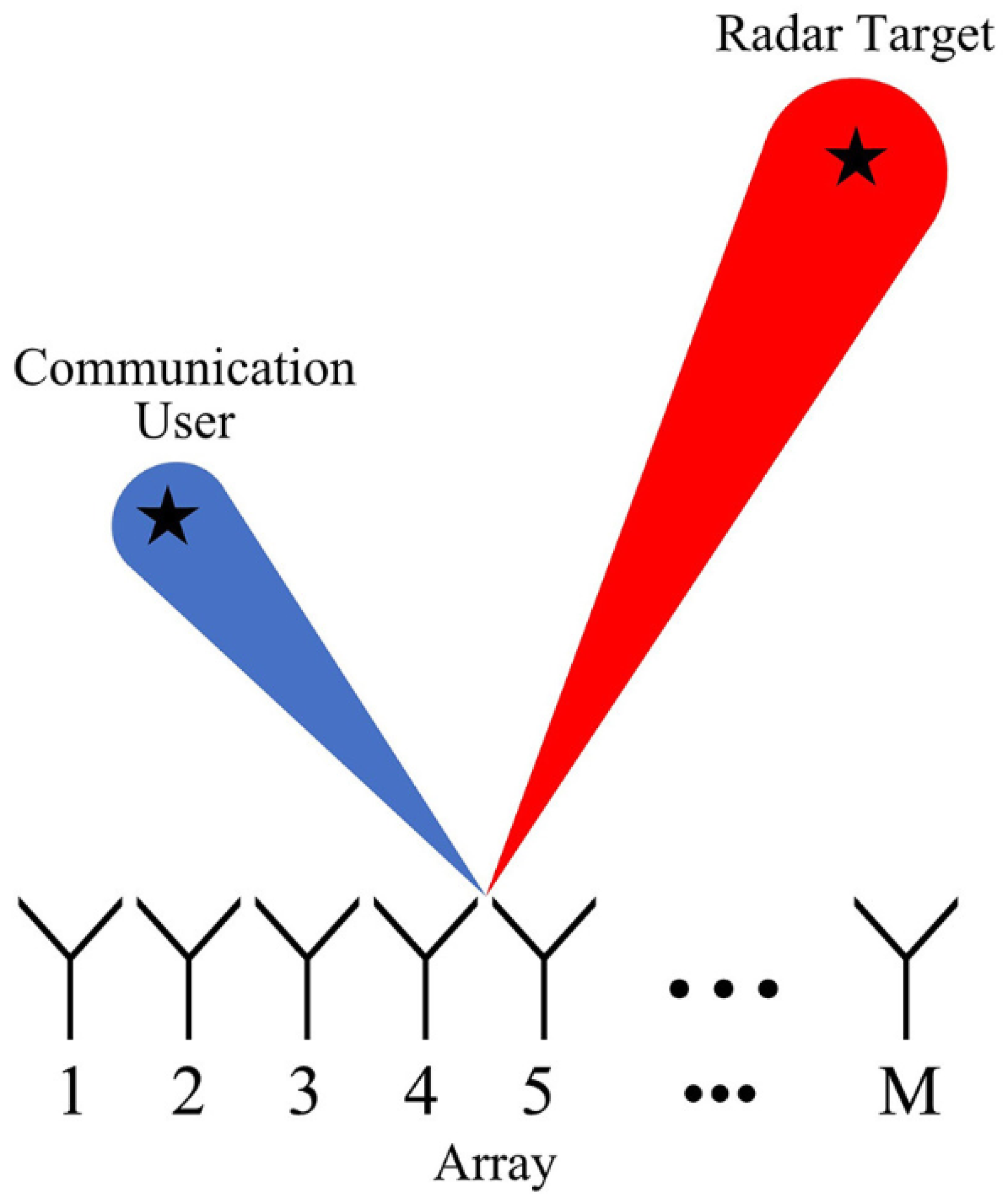
2.1. Multibeam Waveform Strategy

Consider a JRC system equipped with an M-channel uniform linear array (ULA), as shown in Figure 1. The transmitter can employ this array to synthesize the desired radar waveform in one direction and an information-carrying communication waveform in another direction during the same duration and bandwidth. The two desired waveforms work together to simultaneously complete the communication and radar tasks.
Assume that the sampled waveform emitted by the m-th element is x m n , for m = 1 , , M and n = 0 , , N 1 , where N is the number of samples. Let
x n = x 1 n x M n T . Under the narrowband assumption, the far-field synthesized waveform in direction θ can be defined as
s θ , n = a H θ x n ,
where a θ = 1 e j 2 π d   sin   θ λ e j 2 π M 1 d   sin   θ λ T is the steering vector with λ being the waveform carrier wavelength and d being the array element spacing, · T and · H are the transpose and conjugate transpose, respectively.
When direction θ = θ r , the synthetic waveform should be identical to the desired radar waveform s r . When direction θ = θ c , the synthetic waveform should be equal to the desired communication waveform s c . This can be formulated as
a H θ r X = s r T ,
a H θ c X = s c T .
where X = x 0 x N 1 is the transmit waveform matrix composed of all samples of M channels.
Further sorting, (2) and (3) can be succinctly expressed as
A H X = S ,
where A = a θ r a θ c is the collection of spatial steering vectors and S = s r s c T is the collection of desired waveforms.
Under the minimum-norm constraint, the multibeam waveform matrix can be established as
min X X F 2 s . t . A H X = S ,
where · F 2 is the squared-Frobenius norm. The optimization model in (5) is convex and has the close-form solution
X 0 = A A H A 1 S .
where ( ) 1 is the matrix inversion.
The waveform X 0 can synthesize the desired waveforms with the minimum power in direction θ r and θ c .

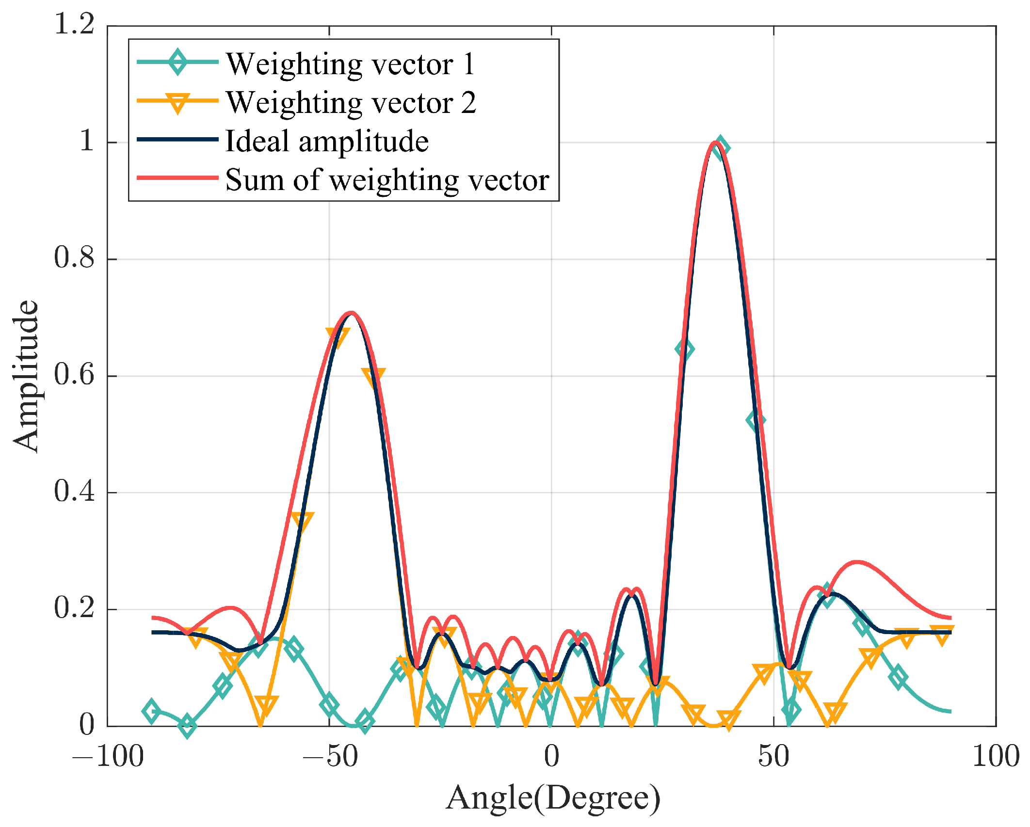
2.2. Spatial Waveform Distribution

When all of the channels transmit the same waveform, the transmit beampattern pointing to θ is generated by employing the beamforming vector in the corresponding direction. In the multibeam strategy, only synthetic waveforms in two directions are assigned. The waveform in each channel is different. It is unknown how the waveform behaves in other directions. We make the mathematical derivation to examine the waveform in any direction. Additionally, spatial emission power is discussed to judge whether the main beams are formed.
When the integrated waveform X is transmitted by the ULA, the synthetic waveform in direction θ is expressed as
s t = a θ T · X ,
The waveform expression can be expanded by substituting (6)
s t = a θ T · X = a θ T A A H A 1 S = v 1 · v 2 · S ,
where v 1 = a θ T A and v 2 = A H A 1 . To simplify the analysis, the formula analysis is carried out item by item.
v 1 = a θ T A = 1 exp j 2 π M 1 d   sin   θ λ a r a c = 1 exp j 2 π M 1 d   sin   θ λ 1 1 exp j 2 π M 1 d sin θ r λ exp j 2 π M 1 d sin θ c λ = m = 0 M 1 exp j 2 π m d sin θ sin θ r λ m = 0 M 1 exp j 2 π m d sin θ sin θ c λ = v 1 , r v 1 , c ,
v 2 = A H A 1 = a r H a c H a r a c 1 = M a r H a c a c H a r M 1 = 1 M 2 a rc a rc * M a rc a rc * M ,
where
a rc = a r H a c = 1 exp j 2 π f 0 M 1 d sin θ r c 1 exp j 2 π f 0 M 1 d sin θ c c = m = 0 M 1 exp j 2 π f 0 m d sin θ r sin θ c c ,
The multiplication result of item v 1 in (9) and item v 2 in (10) represents the weighting factor of the desired radar waveform and desired communication waveform. It determines the spatial synthetic waveform performance and power distribution. The expression for multiplying two items is
v 1 v 2 = 1 M 2 a rc a rc * · v 1 , r v 1 , c M a rc a rc * M = 1 M 2 a rc a rc * · v 1 , r M v 1 , c a rc * v 1 , c M v 1 , r a rc ,
Now we discuss the range of two weighting factors in (12)
v 1 , r M v 1 , c a rc * = M · m = 0 M 1 exp j 2 π f 0 m d sin θ sin θ r c m = 0 M 1 exp j 2 π f 0 m d sin θ sin θ c c m = 0 M 1 exp j 2 π f 0 m d sin θ c sin θ r c = exp j π M 1 d sin θ sin θ r λ · M · sin π M d sin θ sin θ r π M d sin θ sin θ r λ λ sin π d sin θ sin θ r π d sin θ sin θ r λ λ a rc sin π M d sin θ sin θ c π M d sin θ sin θ c λ λ sin π d sin θ sin θ c π d sin θ sin θ c λ λ ,
v 1 , c M v 1 , r a rc = M · m = 0 M 1 exp j 2 π f 0 m d sin θ sin θ c c m = 0 M 1 exp j 2 π f 0 m d sin θ sin θ r c m = 0 M 1 exp j 2 π f 0 m d sin θ r sin θ c c = exp j π M 1 d sin θ sin θ c λ · M · sin π M d sin θ sin θ c π M d sin θ sin θ c λ λ sin π d sin θ sin θ c π d sin θ sin θ c λ λ a rc sin π M d sin θ sin θ r π M d sin θ sin θ r λ λ sin π d sin θ sin θ r π d sin θ sin θ r λ λ ,
When θ = θ r , the weighting factor v 1 , r M v 1 , c a rc * = M 2 a rc 2 is maximum, the other weighting vector v 1 , c M v 1 , r a rc = 0 , and the synthetic waveform is the desired one corresponding to direction θ r . The same situation happens when θ = θ c . The weighting factor v 1 , r M v 1 , c a rc * = 0 and v 1 , c M v 1 , r a rc = M 2 a rc 2 . The synthetic waveform is equal to s c . When θ θ r , θ c , the synthetic waveform is the sum of the damaged desired waveforms which have amplitude attenuation and phase delay. Consequently, there is no expected waveform in any direction except for the area near the desired angle.
Assume that the radar waveform and communication waveform have the same amplitude. The weighting vector value indicates the spatial power performance according to the absolute value inequality theorem,
v 1 v 2 · S = 1 M 2 a rc a rc * · v 1 , r M v 1 , c a rc * v 1 , c M v 1 , r a rc · s r s c T 1 M 2 a rc a rc * · v 1 , r M v 1 , c a rc * s r + 1 M 2 a rc a rc * · v 1 , c M v 1 , r a rc s c = s r M 2 a rc a rc * · v 1 , r M v 1 , c a rc * + v 1 , c M v 1 , r a rc ,
where · is the absolute value operation.
According to (13) and (14), the absolute values of the weighting vectors have similar distribution as the sinc function. The maximum value is obtained only in the desired direction. The sum of the two vectors forms two main beams in the desired directions, while the sum is very low in the remaining direction. A numerical simulation of the weighting vector is analyzed to verify the above discussion. The simulation result is illustrated in Figure 2. Moreover, the parameters are configured in Table 1.
Table 1. Simulation parameters.
ParameterValue
Array number10
Element spacing λ /2
Carrier frequency3 GHz
Sampling number1024
Radar direction36.87
Radar 3dB beam width12.69
Desired radar waveformLFM
Baseband bandwidth100 MHz
Pulse width5.12 μ s
Communication direction−45
Communication 3dB beam width14.36
ModulationQPSK
Symbol number64
PSLR upper bounder−6 dB
PSLR lower bounder−11 dB
Main beam power difference3 dB
Main beams region 61.20 , 28.79 22.55 , 51.19
Sidelobe region 90 , 61.20 28.79 , 22.55 51.19 , 90
Iteration number300
These mathematical derivations confirm that the multibeam strategy synthesizes the desired waveform in the specific direction with the additional effect of energy accumulation. Moreover, the synthetic waveform in the remainder of the directions is random and has low-energy compared to the desired waveform, which prevents the leakage of the waveform and transmit power.

3. Integrated Waveform Design

The multibeam strategy can simultaneously form the traditional radar and communication waveforms to implement the corresponding function. Due to the randomness of the communication waveform, the transmit waveform in (6) generally has unacceptable PAPR that reduces the amplification efficiency of non-linear high-power amplifiers. However, the conflict between constant constraint and beampattern performance gives rise to a high SLL. To solve this problem, the integrated waveform design method based on the beamforming algorithm is proposed in this section.

3.1. Integrated Waveform Design Model with Beamforming Algorithm

Following (1), the power of transmitting in direction θ is given by
P θ = 1 N n = 0 N 1 a H θ x n 2 = a H θ Ra θ ,
where
R = 1 N n = 0 N 1 x ( n ) x H ( n ) = 1 N X X H ,
The covariance matrix of X serves as the transform link between the transmit waveform and the beampattern.
The PAPR limitation is implemented to prevent waveform distortion during saturation amplification; the constraint is described as
x m n μ P t P t M M , m = 1 , , M , n = 0 , , N ,
where μ is the PAPR value and P t is the total transmit power.
The transmit waveform matrix X can be acquired by solving the optimization problem based on the minimum SLL criterion under the constraints of waveform synthesis and constant modulus. The optimization model is expressed as
min X a H θ s Ra θ s s . t . R = 1 N X X H A H X = S x m n = P t P t M M ,
where θ s is the discrete set that covers the sidelobe region. The sidelobe region is defined as the entire area excluding the region of the main beams. The main beams include the radar beam width between the first nulls and the communication beam width between the first nulls.
Since the optimization model is non-convex, we divide the processing into two stages: formulating the integrated waveform covariance matrix under a series of constraints, and then optimizing the integrated waveform using the alternating projection algorithm. The following subsections provide detailed explanations of these.

3.2. Waveform Covariance Matrix Design with Beampattern Constraint

In the JRC system, the integrated waveform should simultaneously synthesize the desired radar and communication waveforms. Moreover, the corresponding beampattern has two main beams pointing to the radar and communication directions, respectively. To depress SLL, we use the peak sidelobe ratio (PSLR) to evaluate its performance, where PSLR is the ratio of the highest level of the sidelobe region and the peak value of communications beam
PSLR = max a H θ s Ra θ s a H θ c Ra θ c .
The communication beam, which usually has less power than the radar beam, is chosen to ensure that the sidelobe level is not higher than any main beam. Since it is hard to optimize the integrated waveform directly, we focus on optimizing the waveform’s covariance matrix R in the first step. The formula for the first-stage optimization function is
min R tr R s . t . 10 log 10 a H θ s Ra θ s 10 log 10 a H θ c Ra θ c p inf 10 log 10 a H θ s Ra θ s 10 log 10 a H θ c Ra θ c p sup 10 log 10 a H θ r Ra θ r 10 log 10 a H θ c Ra θ c = Δ P r c 0.5 a H θ r Ra θ r a H θ r l Ra θ r l = 0 0.5 a H θ r Ra θ r a H θ r r Ra θ r r = 0 0.5 a H θ c Ra θ c a H θ c l Ra θ c l = 0 0.5 a H θ c Ra θ c a H θ c r Ra θ c r = 0 R 0 ,
where tr · is the trace of the matrix, p i n f and p s u p denote the PSLR thresholds, Δ P r c is the difference in the main beam power, which is related to the transmission distance, θ r r θ r l determines the 3 dB width of the radar beam and θ c r θ c l determines the 3 dB width of communication beam.
The objective function in equation 21 is aimed at minimizing the transmit power. The first and second constraints limit the range of PSLR fluctuation. It is a suboptimal result compared with the minimized PSLR condition. It is, nevertheless, the optimal option for the multibeam strategy. In [44], it has been demonstrated that the constant modulus causes a false peak in the sidelobe region. Consequently, these constraints disperse the false peak power to the whole sidelobe region by setting up the PSLR range. The beampattern that matches the constant modulus is acquired in advance. The third constraint sets the power difference between the desired radar waveform and the desired communication waveform. The fourth constraint to the seventh constraint determines the 3dB beam width of the radar beam and communication beam. It has the same performance as the ideal multi-beampattern. The eighth constraint displays that the covariance matrix is the positive semidefinite matrix which is determined by definition. The optimization problem in (21) is convex and can be solved directly by the primal-dual interior point method. The optimal covariance matrix is denoted as R 0 .

3.3. Integrated Waveform Optimization with Alternating Projection Algorithm

After obtaining the optimal covariance matrix R 0 , the integrated waveform X is optimized to minimize the mean square error between the estimated covariance matrix and the optimal one. The objective function is expressed as
f X = R 0 1 N X X H F 2 .
Notice that f X is a 4-order non-convex function that may be tricky to handle. It is worth celebrating that when f = 0, it can be simplified as [48]
f = X N R 0 1 / 2 U F 2 ,
where U C M × N is a unitary matrix satisfying U U H = I M N .
The second-stage optimization problem of X , combined with (23) and the constraints of waveform synthesis and constant modulus, can be modeled as
min X , U X N R 0 1 / 2 U F 2 , s . t . A H X = S x m n = P t P t M M . U U H = I M N .
The optimization problem in (24) is non-convex since the constant modulus and unitary matrix constraints are non-convex sets. We adopt the alternating projection algorithm to solve it in which the optimization problem is disintegrated into a series of simple optimization problems. According to constraints, (24) is decomposed into three sub-problems, which are rewritten as
min X ^ i X ^ i N R 0 1 / 2 U i 1 F 2 s . t . x ^ m i n = P t P t M M ,
min X i X i X ^ i F 2 s . t . A H X i = S ,
min U i X i N R 0 1 / 2 U i F 2 s . t . U i U i H = I M × N ,
where · i means the i-th iteration. These sub-problems have remarkable advantages in that they all have closed-form solutions, and the specific derivations are discussed as follows.
The sub-problem in (25) is a non-convex problem. However, the optimal solution can be given directly according to the amplitude and phase relationship. The result is given by
X ^ i = P t P t M M exp j N R 0 1 / 2 U i 1 .
where · is the phase of complex data.
The sub-problem in (26) is a minimum-norm problem, and its closed-form solution can be obtained by the Lagrange multiplier method. The result is shown as
X i = A A H A 1 S A A H A 1 A H X ^ i + X ^ i .
The sub-problem in (27) is an Orthogonal Procrustes Problem (OPP) [49]. It has a closed-form solution based on Single Value Decomposition (SVD) and is shown as
U i = V r V l H ,
where V l V r H = N X H R 0 1 / 2 , V l C N × M and V r C M × M are unitary matrices corresponding to eigenvalues.
Three sub-problems are iteratively optimized until results meet the convergence conditions or the iteration number reaches the maximum. For ease of description, the proposed method is called the BF-SLL method and is summarized in Algorithm 1.
Remotesensing 15 01167 i001

4. Performance Metrics

In this section, some metrics are defined to evaluate the performance of the proposed method.

4.1. Beampattern Performance Metrics

In the multibeam strategy, two main beams are established to perform radar and communication functions, respectively. The sidelobe region is expected to have low SLL to avoid producing interference. Consequently, the performance of the whole beampattern directly affects the realization of the tasks. We adopt the peak of the main beam, 3 dB main beam width, PSLR, and integrated sidelobe ratio (ISLR) to evaluate it.
The peaks are the value P r in the radar direction θ r and the value P c in the communication direction θ c . High peak values indicate high-power efficiency when the transmit power is the same. Aside from that, the high peak value indicates a high signal-to-noise ratio (SNR) at the same distance in space.
The 3dB main beam widths also include the 3 dB radar beam width B W r and the 3 dB communication beam width B W c . Since no method involves the beam width design, they are expected to be equal to the ideal beam widths
BW = 0.886λ M d cos θ ,
where θ is the main beam direction.
PSLR and ISLR are both used to estimate the sidelobe level. The PSLR is already defined in (20). It measures the relative level between the highest SLL and the main beam. A high PSLR shows that the worthless waveform consumes an amount of transmission power. The high PSLR may even make the transmit array position expose. ISLR describes the efficiency of the transmit power. The ISLR is defined as
ISLR = 10 log 10 E s E m ,
where E s is the power of the whole sidelobe region θ s , and E m is the sum power of two main beams θ m .

4.2. Radar Performance Metrics

From (13) and (14), it can be known that the synthetic waveform varies in different directions. To analyze the radar waveform distribution in the radar beam, the synthetic waveform is filtered to match the desired radar waveform. The impulse response width (IRW), matched filtering PSLR (MF-PSLR), and matched filtering ISLR (MF-ISLR) are utilized to estimate the similarity with the desired radar waveform. IRW is the 3dB width of the main beam. The maximum sidelobe to main beam ratio is defined as the MF-PSLR. MF-ISLR is the ratio of the power of the remaining region except for the first null beam width to the power of the first null beam width.
Besides the matched filtering, noise equivalent sigma zero (NESZ) is another significant metric to evaluate the radar performance. Based on the radar equation, the NESZ is defined as
NESZ = 4 π 3 R 4 F n k T 0 B n P t G 2 λ 2 ,
where R is the waveform emission range, F n is the system noise figure, k = 1 . 38 × 10 23 J/K is the Boltzmann constant, T 0 = 290 K is the standard noise temperature, B n is the noise bandwidth which is equal to the waveform bandwidth, P t is the transmit power, and G is the transmit or receive antenna gain. The transmit power is associated with the PAPR of the integrated waveform [50]. When the PAPR is close to 1, the synthetic waveform has the maximum transmit power.

4.3. Communication Performance Metrics

Bit error ratio (BER) is used to determine communication similarity while analyzing the transmission waveform distribution. Since security is a crucial requirement for communication application, the synthetic waveform is decoded in the entire direction.
SNR is another crucial metric that has an impact on communication performance. The high SNR reveals the low BER. Under the same parameter configuration, the SNR is associated with the transmission distance. Therefore, we examine how the BER degrades with the range in the communication beam.

4.4. Convergence and Computational Complexity Performance

In the BF-SLL method, the first stage is a convex function, which can be computed instantly. The convergence is not affected by this stage. The second stage is non-convex and adopts the alternating projection algorithm to optimize the integrated waveform. The function is divided into three suboptimal problems according to the constraints. Each projection minimizes the error of the iteration variable. Based on the error reduction algorithm [51], the error is non-increasing,
X ^ i + 1 X U i F 2 X U i X i F 2 X i X ^ i F 2 ,
where X U = N R 0 1 2 U i .
Consequently, the proposed method is converged until the convergence metric is met. To compare the convergence speeds of different methods, the normalized iteration error is defined as
δ = X i X i 1 F 2 X i F 2 .
Additionally, the computational complexity of the proposed and conventional algorithms is analyzed. In the proposed algorithm, the computational complexity is mostly determined by the SVD operation and matrix multiplication. The specific value is expressed as O M 2 N I opt , I opt is the total number of iterations. In unit time, the computational complexity is proportional to the communication rate. The computational complexities of the FFRED method in [44] and the AP method in [46] are also expressed as O M 2 N I opt . Despite having the same expression, these three approaches’ varying convergence speeds lead to various I opt in real-world applications. In the IO-AW method [47], the computational complexity is expressed as O M 3 + K 3 + M 2 K + M K 2 N 3 I opt , where K is the number of radar targets and communication users. Typically, K in this paper equals 2. Since this method adopts matrix vectorization, it is much more complicated than other approaches. Naturally, extreme complexity is traded for SLL minimization.

5. Numerical Results

To verify the effectiveness of the proposed method, several simulation and semi-physical results are presented in this section. Simulation results compare the performance metrics of the proposed BF-SLL method, the FFRED method in [44], the AP method in [46], and the IO-AW method in [47]. The results demonstrate that the BF-SLL method has good transmit beampattern performance and synthetic waveform performance. Furthermore, a semi-physical experiment utilizes the digital array transceiver system to complete waveform self-loopback verification. The results prove the proposed method is physically realizable.

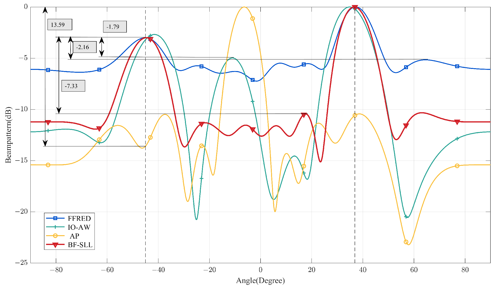
5.1. Simulation Results

In this subsection, we conduct the simulations with an M = 10 element ULA whose element spacing is d = λ /2. The emitted beampattern is expected to have a radar beam towards θ r = 36 . 87 and a communication beam towards θ c = 45 which is 3 dB less than the radar beam power. Furthermore, the beam width is equal to the theoretical value. The desired radar waveform is an up-chirped LFM waveform with bandwidth B = 100 MHz and pulse width T = 5.12 μ s. The desired communication waveform is modulated with quadrature phase shift keying (QPSK) to convey 64 symbols. The upper bound of the PSLR threshold is −6 dB, while the lower bound of the PSLR threshold is −11 dB. In each iteration, the maximum number of iterations is 300. The parameter setting is summarized in Table 1.
Without loss of generality, the proposed method is compared with the FFRED method, the IO-AW method, and the AP method under the same parameters. In the FFRED method, the orthogonal power percentage is required to satisfy the waveform constraints. Through plenty of simulations, the minimum percentage is selected as 54% with the guarantee of waveform synthesis constraint. In the IO-AW method, the initial value uses the waveform matrix that can form a beampattern with the lowest SLL. In the AP method, the desired radar waveform is set only in one direction, similar to other methods. The closed-form solution is obtained by linear superposition.
Figure 3 investigates the transmit beampatterns formed by these four methods. The beampatterns are normalized by the peak value of the radar beam. The simulation results are presented in Table 2. It can be seen that the BF-SLL method forms an excellent beampattern with low SLL and high peaks for each beam. Before normalization, the radar peak value P r of the BF-SLL method is 17.29 dB, which is 2.57 dB higher than that of the FFRED method, 0.92 dB higher than that of the IO-AW method, and 9.02 dB higher than that of the AP method. The same situation also occurs in the communication beam. All of these methods cause the extension of the 3dB beam width, but the proposed method has the minimum extent of deterioration. Another significant feature of the BF-SLL method is the lowest PSLR at −7.33 dB, while the FFRED method formulates a PSLR at -2.16 dB, the IO-AW method formulates a PSLR at −1.79 dB, and the AP method formulates a PSLR at 13.59 dB. It can be further calculated that the ISLR of the BF-SLL method is −13.42 dB, which is 9.70 dB lower than that of the FFRED method, 2.33 dB lower than that of the IO-AW method, and 30.20 dB lower than that of the AP method. This is intuitive that the BF-SLL method allocates more energy to the radar and communication directions and thereby increases the power efficiency. The FFRED method achieves a smooth and stable distribution of the sidelobe region in this parameter configuration, while the BF-SLL method achieves a better one with lower levels. Note that the IO-AW method performs poorly due to the “mirror lobe”, although the remaining sidelobe has an attendant reduction. The high “mirror lobe” equates to a high SNR for the enemy, resulting in an increased detection probability. Although the AP method forms the multi-beampattern to perform the radar and communication functions, it has no more limit on the sidelobe region. The constant constraint causes unacceptable destruction to the beampattern.
Table 2. Results of the beampattern performance metrics.
MethodRadar Peak (dB)Comm. Peak (dB)Radar Beam WidthComm. Beam WidthPSLR (dB)ISLR (dB)
FFRED14.7211.7215.6028.70−2.16−3.72
IO-AW16.3713.3715.9017.80−1.79−11.08
AP8.275.2729.0059.5013.5916.78
BF-SLL17.2914.2913.2015.60−7.33−13.42
Figure 4 illustrates the spatial distribution of radar waveform versus spatial angle θ r ± 7 by using IRW, MF-PSLR, and MF-ISLR as evaluation indexes. Matched filtering is performed on the synthetic waveforms by taking the desired radar waveform as the reference waveform. The curve illustrates the waveform robustness concerning the spatial diversity with no noise. Figure 4a compares the IRW of different methods versus the direction. The IO-AW method shows excellent stability compared to other methods. The maximum fluctuation of others is less than 0.1 μ s, which can roughly be ignored. In Figure 4b, MF-PSLR of the IO-AW method still has stable performance. Unexpectedly, the MF-PSLR of the BF-SLL method in the left region is lower than the ideal value. However, the FFRED method and the AP method experienced intolerable deterioration. The same results of the MF-ISLR are presented in Figure 4c.
Furthermore, Figure 5 displays the matched filtering results of different directions in detail. Except for the radar direction 36 . 87 , the results of other directions almost have the SLL lifting while the main lobe changes little. These results may be explained by the fact that the synthetic waveform is the weighted superposition of the desired radar waveform and the desired communication waveform in (8). As a result, the synthetic waveform in the radar beam exhibits good matched filtering performance. The communication waveform mainly causes the deterioration of the side lobe level.
Figure 6 presents the NESZ versus the range of these four methods. When SNR is equal to 0 dB, the system noise figure is 3 dB, and the antenna gain is 15 dB, we can obtain the NESZ expression according to the radar equation. When the NESZ threshold is −15 dB, the BF-SLL method can transmit 60 meters more than the IO-AW method, 150 meters more than the FFRED method, and 440 meters more than the AP method. Against the background of radar application, the greater the distance, the greater the initiative. Trades an angle saying that the BF-SLL method supports the maximum dynamic range of echo signals because it has the smallest NESZ than the others at the same distance.
The performance of BER has shown in Figure 7. The curve illustrates the waveform robustness concerning the spatial diversity with no noise. All methods eliminate radar waveform interference in the communication direction with zero BER. It can be seen that the BF-SLL method has the best ability to deal with the spatial angle in the communication beam. Additionally, the BF-SLL method outperforms the other three methods in terms of overall spatial directions and has a stable BER distribution.
Figure 8 further demonstrates the performance of BER versus the range over 2000 Monte Carlos. The system parameters are the same as the NESZ simulation. We examine the connection between range, SNR, and BER. The BER of the four methods are roughly equivalent under the same SNR condition, but their corresponding propagation distances are not. The BF-SLL method has the excellent ability to deal with range. When the transmit distance is equal to 800 meters, the BF-SLL method still obtains BER close to the acceptable threshold of the system, while other methods could not. That is to say, the BF-SLL method enables the communication system to have the robust ability to capture long-distance waveforms.
Figure 9 eventually illustrates the convergence speed of these methods. We compare the difference in the results of adjacent iterations and draw two observations: (1) the BF-SLL method will be converged when the number of iterations is large enough; (2) The convergence speed of the BF-SLL method is faster than the IO-AW method but slower than the FFRED method and the AP method. When the convergence condition is set as the normalized iteration error less than 10 4 , the BF-SLL method requires 109 iterations, while the FFRED method requires 90 iterations, the AP method requires 59 iterations, and the IO-AW method requires 242 iterations. This result can be explained by the fact that the transmit power, which is not limited to the FFRED and AP methods, and supplies more freedom for the waveform design.

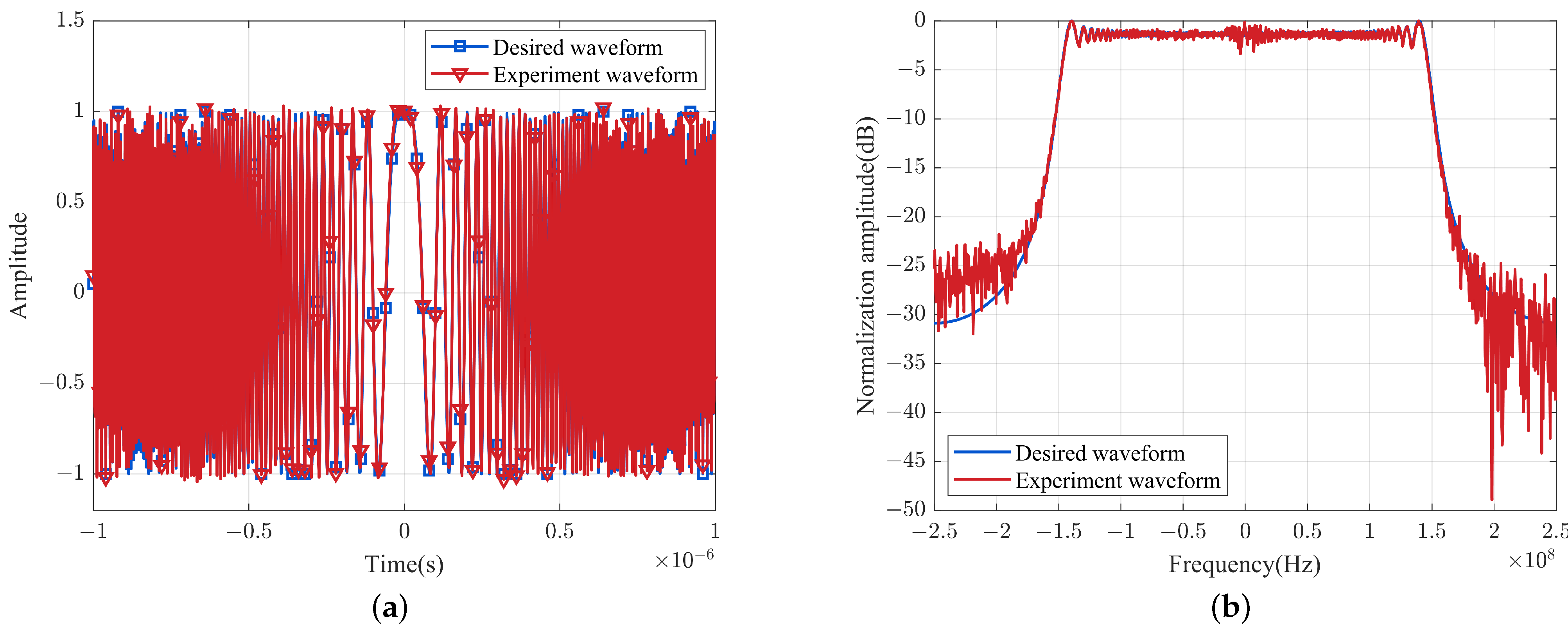
5.2. Semi-Physical Results

In this section, some semi-physical results are performed to show the physical realizability of the proposed method. A digital array transceiver system which consists of eight transmitting channels and one receiving channel is employed to experiment, as shown in Figure 10. The transmitting arrays and the receiving antenna are satisfied with the far-filed assumption. Synthetic waveforms from various directions can be captured by turning the transmitting array’s turntable. Table 3 displays the parameters utilized in the semi-physical experiments.
Table 3. Simulation parameters.
ParameterValue
Array number8
Element spacing0.045 m
Carrier frequency3 GHz
Radar direction 0
Radar 3dB beam width 12 . 69
Desired radar waveformLFM
Baseband bandwidth300 MHz
Pulse width2.048 μ s
Communication direction 45
Communication 3dB beam width 17 . 95
ModulationQPSK
Symbol number64
PSLR upper bounder−4 dB
PSLR lower bounder−12 dB
Main beam power difference3 dB
Main beam region 65.26 , 24.74 14.32 , 14.32
Sidelobe region 90 , 65.26 24.74 , 14.32 14.32 , 90
Iteration number300
Figure 11 presents the experimental radar waveform in the time and frequency domain. Except for a minor wobble at low frequency, the experiment waveform can be seen to be comparable to the desired one. This inconsistency may be due to system interference. For the experimental study of semi-physics, it is permissible. The experimental communication waveform is shown in Figure 12. Similar to Figure 11, the experiment waveform exhibits slight shaking around the desired one. While, the BER keeps at zero, free from shake interference.
A variety of typical directions are chosen to examine the spatial distribution of waveform and power. The findings of the preliminary analysis of the transmit power are shown in Figure 13. The proposed method creates a low-SLL beampattern with a PSLR of −6.68 dB. The semi-physical result, meanwhile, exhibits the same behavior as the simulation result. Following that, Figure 14 and Figure 15 analyze the waveform performances. ISLR and BER are adopted as evaluation metrics by performing the matched filtering and the communication decode operations. It can be seen that the synthetic waveforms emerge with good robustness in the main beam. Unfortunately, the semi-physical experimental results and simulation results at some positions in the sidelobe region exist in deviation, although they do not perform functions. It seems possible that these results are due to the randomness and low power of the synthetic waveform.

6. Discussion

In the previous sections, the BF-SLL method is proposed to simultaneously synthesize the desired waveforms with the low SLL beampattern. Simulation and semi-physical experiment results demonstrate the effectiveness of the proposed method. In the optimization Model (19), the waveform synthesis constraint is the chief constraint, which is the foundation to realize simultaneously radar and communication functions. The multifunction realization can only be guaranteed when the desired functional waveform is synthesized. Therefore, the waveform synthesis constraint is maintained throughout all references. In addition, the data stream and modulations are connected to the waveform synthesis constraint. While the function requirement changes, the integrated waveform needs to update to satisfy it. The objective function minimizes the SLL of the whole sidelobe. It differs from maximizing the power on the two main beams. The deterioration of the sidelobe is caused by the constant modulus constraint which needs more power to provide design freedom. Although the main beams have the maximum power, there is possible to form a false peak in the sidelobe region. We expect to disperse the false peak power to the sidelobe region to decrease the SLL (e.g., Equation (21)).
The optimization Model (21) aims to obtain the waveform covariance matrix corresponding to the low SLL beampattern. The waveform covariance matrix is related to the power difference between the desired radar waveform and the desired communication waveform. There is little relation between the covariance matrix and the specific style of the desired waveform. Equation (21) is convex and can be computed by the convex toolbox. Regarding the generic toolbox’s slow optimization speed, we can design a customized primal-dual interior point method. The Karush–Kuhn–Tucker (KKT) conditions of (21) is expressed as
I M + t 2 t 1 a θ s a H θ s a H θ s Ra θ s a θ c a H θ c a H θ c Ra θ c + v 1 a θ r a H θ r a H θ r Ra θ r a θ c a H θ c a H θ c Ra θ c + v 2 a θ r a H θ r 2 a θ r l a H θ r l + v 3 a θ r a H θ r 2 a θ r r a H θ r r + v 4 a θ c a H θ c 2 a θ c l a H θ c l + v 5 a θ c a H θ c 2 a θ c r a H θ c r Z = 0 ,
t 1 0 , t 2 0 , Z 0 ,
10 log 10 a H θ r Ra θ r 10 log 10 a H θ c Ra θ c = Δ P r c 0.5 a H θ r Ra θ r a H θ r l Ra θ r l = 0 0.5 a H θ r Ra θ r a H θ r r Ra θ r r = 0 0.5 a H θ c Ra θ c a H θ c l Ra θ c l = 0 0.5 a H θ c Ra θ c a H θ c r Ra θ c r = 0 ,
10 log 10 a H θ c Ra θ c 10 log 10 a H θ s Ra θ s p inf 0 10 log 10 a H θ s Ra θ s 10 log 10 a H θ c Ra θ c p sup 0 R 0 ,
t 1 10 log 10 a H θ c Ra θ c 10 log 10 a H θ s Ra θ s p inf = 0 t 2 10 log 10 a H θ s Ra θ s 10 log 10 a H θ c Ra θ c p sup = 0 tr ZR = 0 .
where Z , t 1 , t 1 , v i i = 1 , , 5 are the dual variables. By employing this customized optimization algorithm, the optimization problem can be solved quickly to save computational time.
For communication performance, multipath is a big issue in the real-world communication environment. According to the existing findings, the proposed method can be applied in the multipath environment for the following reasons. The desired communication waveform s c in Equation (3) can adopt any modulation mode. For example, s c can be modulated with OFDM to combat multipath interference. Moreover, the proposed method can only complete the information transmission ability in the line-of-sight direction, while the synthetic waveform in the remaining direction is random and the transmit power is low (seen in Figure 7 and Figure 15). Consequently, the waveform that takes multiple paths to the receiving antenna cannot convey information or cause serious interference. We will verify this performance in future work.

7. Conclusions

In this study, we propose a two-stage transmit waveform design method for the JRC system to synthesize the radar and communication waveforms in desired directions simultaneously. The beamforming algorithm is introduced concerning the high SLL problem to consider the spatial resources and waveform comprehensively. Finally, simulation results demonstrate that the proposed method obtains creditable synthetic waveforms and beampattern performance compared with the FFRED, IO-AW, and AP methods. Additionally, semi-physical experiments are further performed to present the effectiveness and practicability of the proposed BF-SLL method. The following work will consider the links between the integrated waveform design and the communication channel. Moreover, reducing the computational complexity of the algorithm will also be considered.

Author Contributions

L.L. and X.L.; Methodology, L.L. and Y.L. (Yanlei Li); Software, L.L. and M.W.; Validation, Y.L. (Yanlei Li) and Y.L. (Yunlong Liu); Formal analysis, L.L., X.L. and Y.L. (Yanlei Li); Investigation, L.L. and Y.L. (Yunlong Liu); Resources, X.L., X.B. and M.W.; Data curation, L.L. and Y.L. (Yunlong Liu); Writing—original draft, L.L.; Writing—review & editing, X.L., Y.L. (Yanlei Li) and X.B.; Project administration, X.L. and Y.L. (Yanlei Li). All authors have read and agreed to the published version of the manuscript.

Funding

This research received no external funding.

Data Availability Statement

The data presented in this study are available upon request from the corresponding author.

Conflicts of Interest

The authors declare no conflict of interest.

Abbreviations

The following abbreviations are used in this manuscript:
BERBit error ratio
CACyclic algorithm
FHFrequency-hopping
FFREDFar-field radiated emission design
IO-AWIterative optimization with amplitude weighting
IRWImpulse response width
ISLRIntegrated sidelobe ratio
JRCJoint radar-communication
KKTKarush–Kuhn–Tucker
LFMLinear frequency modulation
MF-ISLRMatched filtering integrated sidelobe ratio
MF-PSLRMatched filtering peak sidelobe ratio
MUIMulti-user interference
NESZNoise equivalent sigma zero
OFDMOrthogonal frequency division multiplexing
OPPOrthogonal Procrustes Problem
PAPRPeak-to-average ratio
PSLRPeak sidelobe ratio
QPSKQuadrature phase shift keying
SINRSignal-to-interference-plus-noise ratio
SLL         Sidelobe level
SNRSignal-to-noise ratio
SVDSingle Value Decomposition
ULAUniform linear array

References

  1. Axell, E.; Leus, G.; Larsson, E.; Poor, H. Spectrum sensing for cognitive radio : State-of-the-art and recent advances. IEEE Signal Process. Mag. 2012, 29, 101–116. [Google Scholar]
  2. Geng, Z.; Deng, H.; Himed, B. Adaptive radar beamforming for interference mitigation in radar-wireless spectrum sharing. IEEE Signal Process. Lett. 2015, 22, 484–488. [Google Scholar]
  3. Labib, M.; Marojevic, V.; Martone, A.F.; Reed, J.H.; Zaghloui, A.I. Coexistence between communications and radar systems: A survey. Radio Sci. Bull. 2017, 2017, 74–82. [Google Scholar]
  4. Zheng, L.; Lops, M.; Eldar, Y.C.; Wang, X. Radar and communication coexistence: An overview: A review of recent methods. IEEE Signal Process. Mag. 2019, 36, 85–99. [Google Scholar]
  5. Alaee-Kerahroodi, M.; Raei, E.; Kumar, S.; Shankar, B. Cognitive Radar Waveform Design and Prototype for Coexistence with Communications. IEEE Sens. J. 2022, 22, 9787–9802. [Google Scholar]
  6. Li, B.; Petropulu, A.P.; Trappe, W. Optimum co-design for spectrum sharing between matrix completion based MIMO radars and a MIMO communication system. IEEE Trans. Signal Process. 2016, 64, 4562–4575. [Google Scholar]
  7. Qian, J.; Liu, Z.; Lu, Y.; Zheng, L.; Zhang, A.; Han, F. Radar and communication spectral coexistence on moving platform with interference suppression. Remote Sens. 2022, 14, 5018. [Google Scholar]
  8. Sodagari, S.; Khawar, A.; Clancy, T.C.; McGwier, R. A projection based approach for radar and telecommunication systems coexistence. In Proceedings of the 2012 IEEE Global Communications Conference (GLOBECOM), Anaheim, CA, USA, 3–7 December 2012. [Google Scholar]
  9. Mahal, J.A.; Khawar, A.; Abdelhadi, A.; Clancy, T.C. Spectral Coexistence of MIMO Radar and MIMO Cellular System. IEEE Trans. Aerosp. Electron. Syst. 2017, 53, 655–668. [Google Scholar]
  10. Ma, D.; Shlezinger, N.; Huang, T.; Liu, Y.; Eldar, Y.C. Joint radar-communication strategies for autonomous vehicles: Combining two key automotive technologies. IEEE Signal Process. Mag. 2020, 37, 85–97. [Google Scholar]
  11. He, Q.; Wang, Z.; Hu, J.; Blum, R.S. Performance gains from cooperative MIMO radar and MIMO communication systems. IEEE Signal Process. Lett. 2019, 26, 194–198. [Google Scholar]
  12. Chalise, B.K.; Amin, M.G.; Himed, B. Performance Tradeoff in a Unified Passive Radar and Communications System. IEEE Signal Process. Lett. 2017, 24, 1275–1279. [Google Scholar]
  13. Zhang, J.A.; Rahman, M.L.; Wu, K.; Huang, X.; Guo, Y.J.; Chen, S.; Yuan, J. Enabling joint communication and radar sensing in mobile networks—A survey. IEEE Commun. Surv. Tutor. 2022, 24, 306–345. [Google Scholar]
  14. Zhang, Z.; Chang, Q.; Yang, S.; Xing, J. Sensing-communication bandwidth allocation in vehicular links based on reinforcement learning. IEEE Wirel. Commun. Lett. 2022, 12, 1. [Google Scholar]
  15. Liyanaarachchi, S.D.; Riihonen, T.; Barneto, C.B.; Valkama, M. Optimized waveforms for 5G–6G communication with sensing: Theory, simulations and experiments. IEEE Trans. Wirel. Commun. 2021, 20, 8301–8315. [Google Scholar]
  16. Wild, T.; Braun, V.; Viswanathan, H. Joint design of communication and sensing for beyond 5G and 6G systems. IEEE Access 2021, 9, 30845–30857. [Google Scholar]
  17. Liu, Y.; Liao, G.; Yang, Zh. Robust OFDM Integrated Radar and Communications Waveform Design Based on Information Theory. Signal Process. 2019, 162, 317–329. [Google Scholar]
  18. Zhang, Q.; Sun, H.; Wei, Z.; Feng, Z. Sensing and communication integrated system for autonomous driving vehicles. In Proceedings of the IEEE INFOCOM 2020-IEEE Conference on Computer Communications Workshops (INFOCOM WKSHPS), Online, 6–9 July 2020. [Google Scholar]
  19. Wang, J.; Liang, X.D.; Chen, L.Y.; Wang, L.N.; Li, K. First demonstration of joint wireless communication and high-resolution SAR imaging using airborne MIMO radar system. IEEE Trans. Geosci. Remote Sens. 2019, 57, 6619–6632. [Google Scholar]
  20. Hassanien, A.; Amin, M.G.; Zhang, Y.D.; Ahmad, F. Signaling strategies for dual-function radar communications: an overview. IEEE Aerosp. Electron. Syst. Mag. 2016, 31, 36–45. [Google Scholar]
  21. Li, Q.; Dai, K.; Zhang, Y.; Zhang, H. Integrated waveform for a joint radar-communication system with high-speed transmission. IEEE Wirel. Commun. Lett. 2019, 8, 1208–1211. [Google Scholar]
  22. Nowak, M.J.; Zhang, Z.; LoMonte, L.; Wicks, M.; Wu, Z. Mixed-modulated linear frequency modulated radar-communications. IET Radar Sonar Navig. 2017, 11, 313–320. [Google Scholar]
  23. Zhang, Z.; Nowak, M.J.; Wicks, M.; Wu, Z. Bio-inspired RF steganography via linear chirp radar signals. IEEE Commun. Mag. 2016, 54, 82–86. [Google Scholar]
  24. Zhang, Z.; Qu, Y.; Wu, Z.; Nowak, M.J.; Ellinger, J.; Wicks, M.C. RF Steganography via LFM Chirp Radar Signals. IEEE Trans. Aerosp. Electron. Syst. 2018, 54, 1221–1236. [Google Scholar]
  25. Liu, Y.; Liao, G.; Xu, J.; Yang, Z.; Zhang, Y. Adaptive OFDM integrated radar and communications waveform design based on information theory. IEEE Commun. Lett. 2017, 21, 2174–2177. [Google Scholar]
  26. Liu, Y.; Liao, G.; Chen, Y.; Xu, J.; Yin, Y. Super-resolution range and velocity estimations with OFDM integrated radar and communications waveform. IEEE Trans. Veh. Technol. 2020, 69, 11659–11672. [Google Scholar]
  27. Sturm, C.; Zwick, T.; Wiesbeck, W. An OFDM System Concept for Joint Radar and Communications Operations. In Proceedings of the VTC Spring 2009-IEEE 69th Vehicular Technology Conference, Barcelona, Spain, 26–29 April 2009. [Google Scholar]
  28. Rong, J.; Liu, F.; Miao, Y. Integrated Radar and Communications Waveform Design Based on Multi-Symbol OFDM. Remote Sens 2022, 14, 1–22. [Google Scholar]
  29. Ahmed, A.; Zhang, Y.D.; Hassanien, A. Joint Radar-communications exploiting optimized OFDM waveforms. Remote Sens. 2021, 13, 4376. [Google Scholar]
  30. Hassanien, A.; Aboutanios, E.; Amin, M.G.; Fabrizio, G.A. A dual-function MIMO radar-communication system via waveform permutation. Digit. Signal Process. 2018, 83, 118–128. [Google Scholar]
  31. Hassanien, A.; Amin, M.G.; Zhang, Y.D.; Ahmad, F. Phase-modulation based dualfunction radar-communications. IET Radar Sonar Navig 2017, 10, 1411–1421. [Google Scholar]
  32. Hassanien, A.; Himed, B.; Rigling, B.D. A dual-function MIMO radar communications system using frequency-hopping waveforms. In Proceedings of the IEEE National Conference on Radar, Seattle, WA, USA, 8–12 May 2017; pp. 1721–1725. [Google Scholar]
  33. Zhang, Q.; Zhou, Y.; Zhang, L.; Gu, Y.; Chen, Z. Application of LFM-CPM signal into a DFRC system based on circulating code array. Digit. Signal Process 2020, 101, 102712. [Google Scholar]
  34. Zhang, Q.; Zhou, Y.; Zhang, L.; Gu, Y.; Zhang, J. Circulating code array for a dual-function radar-communications system. IEEE Sens. J. 2020, 20, 786–798. [Google Scholar]
  35. Zhang, Q.; Feng, C.; Gu, Y.; Zhang, L.; Zhou, Y.; Chen, Z. Transmit beampattern design for joint radar-communications system with circulating code array. Digit. Signal Process. 2022, 127, 103591. [Google Scholar]
  36. Hassanien, A.; Amin, M.G.; Zhang, Y.D.; Ahmad, F. Dual-function radar-communications: Information embedding using sidelobe control and waveform diversity. IEEE Trans. Signal Process. 2016, 64, 2168–2181. [Google Scholar]
  37. Ji, S.; Chen, H.; Hu, Q.; Pan, Y.; Shao, H. A dual-function radar-communication system using FDA. In Proceedings of the 2018 IEEE Radar Conference (RadarConf18), Oklahoma, OH, USA, 23–27 April 2018. [Google Scholar]
  38. Nusenu, S.Y.; Huaizong, S.; Ye, P.; Xuehan, W.; Basit, A. Dual-function radarcommunication system design via sidelobe manipulation based on FDA butler matrix. IEEE Antennas Wirel. Propag. Lett 2019, 18, 452–456. [Google Scholar]
  39. Liu, F.; Zhou, L.; Masouros, C.; Li, A.; Luo, W.; Petropulu, A. Toward dual-functional radar-communication systems: Optimal waveform design. IEEE Trans. Signal Process. 2018, 66, 4264–4279. [Google Scholar]
  40. Liu, F.; Masouros, C.; Griffiths, H. Dual-functional radar-communication waveform design under constant-modulus and orthogonality constraints. In Proceedings of the 2019 Sensor Signal Processing for Defence Conference (SSPD), Brighton, UK, 9–10 May 2019. [Google Scholar]
  41. Liu, F.; Masouros, C.; Ratnarajah, T.; Petropulu, A. On Range Sidelobe Reduction for Dual-Functional Radar-Communication Waveforms. IEEE Wirel. Commun. Lett. 2020, 9, 1572–1576. [Google Scholar]
  42. Liu, X.; Huang, T.; Shlezinger, N.; Liu, Y.; Zhou, J.; Eldar, Y.C. Joint Transmit Beamforming for Multiuser MIMO Communications and MIMO Radar. IEEE Trans. Signal Process. 2020, 68, 3929–3944. [Google Scholar]
  43. Liu, X.; Huang, T.; Liu, Y.; Zhou, J. Constant Modulus Waveform Design for Joint Multiuser MIMO Communication and MIMO Radar. In Proceedings of the Wireless Communications and Networking Conference Workshops (WCNCW), Nanjing, China, 29 March 2021; pp. 1–5. [Google Scholar]
  44. McCormick, P.M.; Blunt, S.D.; Metcalf, J.G. Simultaneous radar and communications emissions from a common aperture, Part I: Theory. In Proceedings of the 2017 IEEE Radar Conference (RadarConf), Seattle, WA, USA, 8–12 May 2017. [Google Scholar]
  45. McCormick, P.M.; Ravenscroft, B.; Blunt, S.D.; Duly, A.J.; Metcalf, J.G. Simultaneous radar and communication emissions from a common aperture, Part II: Experimentation. In Proceedings of the 2017 IEEE Radar Conference (RadarConf), Seattle, WA, USA, 8–12 May 2017. [Google Scholar]
  46. Jiang, M.; Liao, G.; Yang, Z.; Liu, Y.; Chen, Y.; Li, H. Integrated waveform design for an Integrated Radar and Communication System with a Uniform Linear Array. In Proceedings of the 2020 IEEE 11th Sensor Array and Multichannel Signal Processing Workshop (SAM), Hangzhou, China, 8–11 June 2020. [Google Scholar]
  47. Jiang, M.; Liao, G.; Yang, Z.; Liu, Y.; Chen, Y. Integrated radar and communication waveform design based on a shared array. Signal Process. 2021, 182, 107956. [Google Scholar]
  48. Stoica, P.; He, H.; Li, J. New algorithms for designing unimodular sequences with good correlation properties. IEEE Trans. Signal Process. 2009, 57, 1415–1425. [Google Scholar]
  49. Viklands, T. Algorithms for the Weighted Orthogonal Procrustes Problem and Other Least Squares Problems. Ph.D. Thesis, Umea University, Umea, Sweden, 2008. [Google Scholar]
  50. Jiang, T.; Wu, Y. An overview: Peak-to-average power ratio reduction techniques for OFDM signals. IEEE Trans. Broadcast. 2008, 54, 257–268. [Google Scholar]
  51. Bauschke, H.H.; Combettes, P.L.; Luke, D.R. Phase retrieval, error reduction algorithm, and Fienup variants: A view from convex optimization. J. Opt. Soc. Am. A Opt. Image Sci. Vis. 2002, 19, 1334–1345. [Google Scholar]
Figure 1. Multibeam strategy of joint radar communication system.
Remotesensing 15 01167 g001
Figure 2. The absolute value of the weighting vector in different directions.
Remotesensing 15 01167 g002
Figure 3. Transmit beampattern comparison for different methods.
Remotesensing 15 01167 g003
Figure 4. Performance of matched filtering in the radar beam. (a) IRW of different methods. (b) MF−PSLR of different methods. (c) MF−ISLR of different methods.
Remotesensing 15 01167 g004
Figure 5. The synthetic waveform matched filtering results from several angles. (a) Matched filtering result in direction 29 . 87 . (b) Matched filtering result in direction 33 . 87 . (c) Matched filtering result in direction 35 . 87 . (d) Matched filtering result in direction 36 . 37 . (e) Matched filtering result in direction 36 . 87 . (f) Matched filtering result in direction 37 . 87 . (g) Matched filtering result in direction 38 . 87 . (h) Matched filtering result in direction 40 . 87 . (i) Matched filtering result in direction 43 . 87 .
Remotesensing 15 01167 g005aRemotesensing 15 01167 g005b
Figure 6. Noise equivalent sigma zero versus the range of different methods.
Remotesensing 15 01167 g006
Figure 7. Bit error rate (BER) versus spatial angle of different methods.
Remotesensing 15 01167 g007
Figure 8. Bit error rate (BER) versus the range of different methods.
Remotesensing 15 01167 g008
Figure 9. Convergence comparison of different methods by normalized waveform error.
Remotesensing 15 01167 g009
Figure 10. Experimental setup. (a) The transmitting array connects with the transceiver system. (b) Setup of the transmitting array and receiving antenna.
Remotesensing 15 01167 g010
Figure 11. Comparison of the desired synthetic waveform (blue) and the experimental synthetic waveform (red) in radar direction. (a) Comparison in the time domain. (b) Comparison in the frequency domain.
Remotesensing 15 01167 g011
Figure 12. Comparison of the desired synthetic waveform (blue) and the experimental synthetic waveform (red) in communication direction. (a) Comparison in the time domain. (b) Comparison for the phase.
Remotesensing 15 01167 g012
Figure 13. Comparison of the desired beampattern (blue) and the experimental beampattern (red).
Remotesensing 15 01167 g013
Figure 14. Comparison of the desired ISLR (blue) and the experimental ISLR (red).
Remotesensing 15 01167 g014
Figure 15. Comparison of the desired BER (blue) and the experimental BER (red).
Remotesensing 15 01167 g015
Disclaimer/Publisher’s Note: The statements, opinions and data contained in all publications are solely those of the individual author(s) and contributor(s) and not of MDPI and/or the editor(s). MDPI and/or the editor(s) disclaim responsibility for any injury to people or property resulting from any ideas, methods, instructions or products referred to in the content.

