
A Novel Atmospheric Correction for Turbid Water Remote Sensing

1
Marine Science and Technology College, Zhejiang Ocean University, Zhoushan 316022, China
2
Nanjing Institute of Geography & Limnology Chinese Academy of Sciences, Nanjing 210008, China
3
University of Chinese Academy of Sciences, Beijing 100191, China
4
Zhejiang Haida Marine Survey, Planning and Design Co., Ltd., Zhoushan 316022, China
*
Author to whom correspondence should be addressed.
Remote Sens. 2023, 15(8), 2091; https://0-doi-org.brum.beds.ac.uk/10.3390/rs15082091
Submission received: 28 February 2023
/
Revised: 7 April 2023
/
Accepted: 13 April 2023
/
Published: 15 April 2023
(This article belongs to the Special Issue Remote Sensing Retrievals of Optical Properties in Inland Waters and the Coastal Ocean)
Abstract
:For the remote sensing of turbid waters, the atmospheric correction (AC) is a key issue. The “black pixel” assumption helps to solve the AC for turbid waters. It has proved to be inaccurate to regard all water pixels in the SWIR (Short Wave Infrared) band as black pixels. It is necessary to perform atmospheric correction in the visible bands after removing the radiation contributions of water in the SWIR band. Here, the modified ACZI (m-ACZI) algorithm was developed. The m-ACZI assumes the spatial homogeneity of aerosol types and employs the BPI (Black Pixel Index) and PIFs (Pseudo-Invariant Features) to identify the “black pixel”. Then, the radiation contributions of waters in the SWIR band are removed to complete the atmospheric correction for turbid waters. The results showed that the m-ACZI had better performance than the SeaDAS (SeaWiFS Data Analysis System) -SWIR and the EXP (exponential extrapolation) algorithm in the visible band (sMAPE < 30.71%, RMSE < 0.0111 sr−1) and is similar to the DSF (Dark Spectrum Fitting) algorithm in floating algae waters. The m-ACZI algorithm is suitable for turbid inland waters.
1. Introduction
Atmospheric correction (AC) is a key step of ocean color data processing. The “black pixel” assumption is commonly applied to AC for waters (including open ocean, coastal, and inland waters) [1,2,3,4,5,6,7]. The radiance of the “black pixel” is assumed to be dominated by atmospheric radiance, and the contribution from water can be neglected; hence, the AC of satellite images can be completed using the “black pixel” assumption [6,8]. This assumption depends on the fact that the water radiation is dominated by the strong absorption of pure water. Early on, waters in near-infrared (NIR) bands were determined to fit this assumption, and the water-leaving reflectance (ρw) (or the remote sensing reflectance (Rrs)) in the visible bands was derived by removing the aerosol scattering through extrapolation from the NIR bands [6,8,9].
However, follow-up studies showed that the contribution of turbid water in NIR bands could not be neglected [10,11]. The short-wave infrared (SWIR) bands with a longer wavelength and stronger absorption were considered to fit the “black pixel” assumption for turbid waters [9,12,13,14]. Wang et al. (2019) found that the ρw of algae waters was strong in SWIR bands, meaning these bloom waters no longer met the “black pixel” assumption [15]. In Lake Taihu, significant water signals in SWIR bands were detected when algal blooms occurred (Figure 1). Therefore, the contribution of waters in SWIR bands should be removed before the estimation of aerosol scattering in visible bands. Wang et al. (2019) developed the BPI (black pixel index) to obtain the “black pixel” from turbid waters and proposed the ACZI algorithm (atmospheric correction algorithm based on a zero assumption for the short-wave infrared band) for inland turbid waters. The water pixels in the 2201 nm band were considered black pixels by the ACZI algorithm for Landsat 8 images, and aerosol scattering in the visible bands was derived from the assumption of the zero contribution of waters in the 2201 nm band [12]. Figure 1 shows that the Rayleigh-corrected reflectance (ρrc) in SWIR bands is very different in water areas without algal blooms; it is incorrect that all water pixels in the SWIR band are treated as black pixels. It is necessary to obtain the “black pixel” with a more accurate identification method.
Here, we modified the identification method of the “black pixel” in the ACZI algorithm [12], and the m-ACZI algorithm was developed. In the m-ACZI algorithm, the water contribution in SWIR bands was removed using the combination of BPI [12] and PIFs (pseudo-invariant features) [16,17], and accurate aerosol scattering in SWIR bands was derived. This scheme was evaluated in turbid inland waters, with its performance also compared with other AC algorithms.
Figure 1.
(a) False color image (R: SWIR band, G: NIR band, B: Blue band), (b) Algal bloom map derived by FAI (floating algae index) [18,19], and the Rayleigh-corrected reflectance (ρrc) in SWIR bands (c,d) and its histograms from Lake Taihu with algal bloom on 30 January 2021. (e) Average ρrc from three boxes (Z1, Z2, and Z3) without algal blooms.

2. Dataset and Methods
2.1. Satellite Data
The cloudless Landsat8-OLI (Operational Land Imager) Level-1 data were from the USGS (United State Geological Survey) and were processed to the Rrs data via the AC algorithms (details in Section 2.3.2). In this work, three OLI images of Lake Taihu (dates: 11 May 2017, 27 May 2017, and 21 December 2017) were matched with the in situ data to evaluate the performance of the AC algorithms. The time window of data matching was set as ±3 h of the Landsat8 overpass. The AC-driven Rrs data were obtained by averaging a 3 × 3 pixel (the coefficient of variation for these valid pixels was < 10%) area surrounding the sample point location [20,21,22,23]. A total of 71 sampling points were matched (11 match-up points from 11 May 2017; 22 match-up points from 27 May 2017; and 38 match-up points from 21 December 2017) (Figure 2).
2.2. Field Spectral Data
The Rrs was measured using the spectrometer (ASD FieldSpec 4) following NASA (National Aeronautics and Space Administration) Ocean optics protocols [24] (Figure 3):
where Lt is the total water-leaving radiance; ρp is the reflectance; Lg is the radiance of the reference panel; Lsky is the sky radiance; Lw is the water-leaving radiance; and Ed is the downwelling plane irradiance. Additionally, the water surface reflectance factor σ was assumed to be 0.028 [25].
2.3. Methods
2.3.1. The m-ACZI Algorithm
The black pixel of the ACZI algorithm was identified using the combination of BPI (Equation (2)) [12] and FAI (the floating algae index) [18,19], and this algorithm assumed that all water pixels in the 2201 nm band accord with the “black pixel” hypothesis. However, the ρw in SWIR bands was significant and non-negligible when algal blooms occurred (Figure 1). In this study, the m-ACZI algorithm changed ACZI’s black pixel identification method of the black pixels of ACZI to the BPI-PIF combination, and these black pixels are applied to remove the water contribution in SWIR bands. After this stage, the following process is the same as the ACZI algorithm [12]. The BPI was developed by Wang et al. (2019a) [12] to identify the black pixel from turbid waters (Equation (2)). Schott et al. (1988) [17] considered that urban construction land has pseudo-invariant features (PIFs) and proposed the PIF mask method. The BPI and PIF mask followed the methods described by Wang et al. (2019a) [12] and Schott et al. (1988) [17], respectively.
The PIFs are with features that do not change their reflectivity properties drastically over time in a scene [17]. The surface reflectance of PIFs is similar for the two dates. Hence, the difference between the Rayleigh-corrected reflectance (ρrc) of PIFs from two dates can be considered as the difference between two values of aerosol reflectance (ρa) of PIF. The black pixels are pixels consisting only of atmospheric radiance (Rayleigh scattering and aerosol scattering). If a pixel is a true “black pixel”, the difference between its ρrc for two dates is the same as the difference between its ρa for the same two dates (Equations (5)–(7)). Furthermore, theoretically, if the difference in the ρrc of a water pixel between two dates in the SWIR band is equal or approximate to the difference in the ρrc of PIFs between two dates, this water pixel can be taken as a “black pixel”. Therefore, the characteristics of PIFs can be used to more accurately obtain the BPIs for atmospheric correction. The flowchart of the m-ACZI algorithm is shown in Figure 4.
(1) The ρrc and transmittance (t) are obtained from a LUT (lookup table) generated for all OLI bands using 6SV (the vector version of the Second Simulation of the Satellite Signal in the Solar Spectrum) according to sun and sensor geometry [26,27]. The ρrc can be derived from the reflectance of the atmosphere (ρt). The sea surface reflectance from whitecaps and sunglint were ignored [1,2,28,29].
For land pixels:
where ρs is the surface reflectance.
For a water pixel:
(2) Two masks are made by the BPI for two date images (T1 and T2) [4,12], and the overlapped pixels in two masks (BPI mask) are retained. The difference in ρrc (SWIR) for two date images (DBPI) is calculated and masked by the BPI mask.
(3) The PIF mask is extracted according to Schott et al. (2016) [16]. The construction land features are considered as PIFs, and this extraction is applied over the construction area within the image (Figure 5). For PIFs, the ρs is invariable, and the difference in ρrc (SWIR) for two date images (DPIF) is masked by the PIF mask.
Δt will make ρSPIF residual in DPIF and affect the matching of DPIF and DBPI; for this, we analyze and discuss the impact of Δt on DPIF (1609) (details in Section 4.4). The results showed that when Δt was less than 0.0107, the DPIF change caused by Δt was about 2.70%, which is within the allowable error range.
(4) The ρaBPI and ρaPIF are similar in one OLI image based on the assumption of the spatial uniformity distribution of aerosol types. The DBPI matches the mode number of DPIF (with ±10% variation) to obtain the final BPI-PIF mask. The black pixels were identified using the BPI-PIF mask (Example: Figure 6). The aerosol scattering from black pixels is used to remove the water contribution for nonblack pixels.
(5) The atmospheric correction for all water pixels is completed using the same steps as the ACZI algorithm [12], and Rrs (or ρw) data are obtained.
Described below is the process of developing the m-ACZI algorithm.
- (1)
- We extracted the PIF mask according to Schott et al., 1988 [17] and Concha and Schott 2016 [16]. For Lake Taihu, the 2201 nm band with a threshold of 0.05 was used to obtain the water mask, and the threshold of the NIR/RED band ratio was set to 1.3 for obtaining the vegetation mask. The previous two masks were combined using logic. AND. gate, creating a “PIF mask” that rejects the vegetation and water and only accepts the construction land features.
- (2)
- In this step, we calculated the ρrc and t using the 6SV-LUT from ACOLITE (atmospheric correction for OLI lite).
- (3)
- Based on step 2, we adopted the BPI [12] to obtain the BPI mask, and the threshold of the BPI was set to 0~0.1.
- (4)
- Following steps 1, 2, and 3, concerning t values, two images with similar t values were selected to obtain their PIF mask and BPI mask, respectively. Then, these masks were applied to the ρrc (SWIR) images, respectively, to obtain the PIF and BPI images. We subtracted two of each image type to obtain the DPIF and DBPI images.
- (5)
- We counted the average value of DPIF and used the average DPIF with 10% variation as the judgment value for DBPI, i.e., DBPI pixels greater than the average DPIF with 10% variation were discarded.
- (6)
- Following the ACZI process [12], we counted the median value from the final retained DBPI pixels, and this median value was taken as ρa on two SWIR bands. The aerosol scattering ratio (ε), consisting of these two ρa(SWIR) values, was applied to all water pixels, and aerosol scattering in the visible and near-infrared bands was obtained using an exponential extrapolation method, thus completing the final atmospheric correction process to obtain Rrs.
2.3.2. Other Atmospheric Correction Algorithms
The SeaDAS-SWIR Algorithm
For turbid waters, the “black pixel” assumption in NIR bands is invalid because of the contribution of phytoplankton, detritus, and suspended sediment to water backscatter [2,10]. Research from Hale et al. (1973) indicated that the water in SWIR bands has stronger absorption than that in NIR bands [30], and the turbid water in the former meets the requirement of the “black pixel” assumption [13]. Therefore, Wang and Shi (2005) [10] developed an AC algorithm for turbid water based on extrapolation from SWIR bands and integrated this AC algorithm into SeaDAS (SeaWiFS Data Analysis System, referred to as SeaDAS-SWIR in this paper; more details can be found in Wang and Shi (2005) [10]).
The ACOLITE (atmospheric correction for OLI lite; this study worked with version 20211112) tool was developed for coastal and inland waters by the Remote Sensing and Ecosystem Modelling (REMSEM) team. It performs this process using dark spectrum fitting (DSF) and exponential extrapolation (EXP) [14,26,31,32,33].
The EXP Algorithm
The idea of the EXP algorithm is consistent with the SeaDAS-SWIR algorithm, both of which are based on exponential extrapolations of the ratio of multiple aerosol scattering in SWIR bands, but the EXP algorithm does not deal with aerosol LUTs (lookup tables) [14]. The EXP algorithm only uses an exponential extrapolation method to estimate aerosol scattering in visible bands and NIR bands [28].
The DSF Algorithm
The DSF algorithm is presented for meter-scale-resolution optical satellite imagery [26,31]. Similar to other AC algorithms, this algorithm was also developed based on the “black pixel” concept [26]. However, the difference is that it defines black pixels as pixels with zero surface reflection in one scene image, including land pixels and water pixels. These black pixels are employed to estimate the atmospheric radiance for other pixels. It can be seen that the DSF depends on two assumptions: (1) the spatial distribution of the atmosphere is uniform in an image; (2) at least one pixel whose surface reflection is about zero exists in one scene image [26,31].
2.3.3. Algorithm Accuracy Analysis
The root-mean-square error (RMSE), symmetric mean absolute percentage error (sMAPE), and Bias were used to determine the differences between the in situ data and the AC-driven data:
where Ri is the in situ Rrs data, Rm is the OLI-Rrs data via atmospheric correction, and n is the number of match-up pairs.
3. Results
3.1. Assessment of the m-ACZI Algorithm
As Figure 7 and Figure 8 show, the m-ACZI raised the Rrs estimation compared to the ACZI algorithm, so the histograms of Rrs generally moved and concentrated to high value areas (Figure 8). Notably, the m-ACZI algorithm did not increase the Rrs values for all water pixels, but mainly for algal bloom pixels (green pixels in the RGB true-color images) (Figure 2 and Figure 7). It can also be observed that the m-ACZI algorithm reduced the Rrs estimation of the non-algal bloom pixels in the 865 nm band (Figure 7), which were consistent with the characteristics of the in situ Rrs (Figure 3).
Most of the scatterplots of the ACZI were below the 1:1 line, and part of the scatterplots derived in the 865 nm band were above the 1:1 line (Figure 9a). The scatterplots of the m-ACZI were distributed around the 1:1 line, with several significant off-group points in the 865 nm band (Figure 9b). In general, compared with the scatterplots of the ACZI, the scatterplots of the m-ACZI were more concentrated near the 1:1 line. The ACZI-driven Rrs was underestimated in all visible bands. The Rrs derived by the m-ACZI was also underestimated in the 561 nm and 655 nm bands, but overestimated in two BLUE bands (Figure 9 and Table 1). The minimum sMAPE was obtained by the m-ACZI in the 655 nm band, followed by the m-ACZI in the 561 nm band. Similarly, the minimum RMSE was provided by the m-ACZI in the 483 nm band, followed by the m-ACZI in the 443 nm band. However, the minimum bias was obtained from the data derived by the ACZI in the 443 nm band (Table 1). Overall, from RMSE and sMAPE, the m-ACZI was superior to the ACZI in all visible bands, especially in the 561 nm and 655 nm bands; the performance of the m-ACZI algorithm was greatly improved. However, these 2 algorithms still failed in the NIR band (RMSE > 0.0203 sr−1; sMAPE > 48.31%; bias > 88.83%). From the scatterplots of the 865 nm band in Figure 9, these 2 AC algorithms have overestimations. The assessment results indicate that the m-ACZI algorithm is generally better than the ACZI algorithm.
3.2. Comparison with other AC Algorithms
Only 54 match-up sample points were used to evaluate the SeaDAS-SWIR algorithm because some water pixels were masked by this algorithm (the “proc_ocean” option of SeaDAS was set to “2-force all pixels to be processed as ocean”). In Figure 10, the scatterplots of the m-ACZI algorithm were more concentrated, while those of other algorithms were discrete, especially in the 443 nm and 483 nm bands. The scatterplot distributions of the m-ACZI and the DSF were very similar in the 561 nm and 655 nm bands and were closer to the 1:1 line than others (Figure 10). The statistical results of the accuracy also supported these findings (Table 2). The assessment results from the m-ACZI and the DSF were very similar: the RMSE difference between them was less than 0.0008 in visible bands, and both were more accurate than the SeaDAS and the EXP algorithms. It should be noted that all the AC algorithms failed in the NIR band (RMSE > 0.0134 sr−1; sMAPE > 49.31%; Bias > 88.83%), and the m-ACZI algorithm showed the best comprehensive performance.
3.3. Assessment of AC Algorithms for Different Water Types
According to the water classification method of Sun et al. (2012), waters were classified into two types: floating bloom (FB) and un-floating bloom (uFB) [15,34]. Figure 11 shows the scatterplots of Rrs between in situ data and the AC algorithm in different water types, with detailed statistics presented in Table 3 and Table 4. All AC algorithms had more discrete scatterplots in FB than in uFB, especially in the two blue bands, where the bias of the algorithm increased significantly (Table 3 and Table 4). Table 3 shows that the assessment results of the m-ACZI and the DSF algorithms were superior to other algorithms in the uFB. In particular, the m-ACZI and the DSF algorithms showed satisfactory performance in the 561 nm and 655 nm bands (RMSE < 0.0087 sr−1; sMAPE < 19.31%), which was sufficient to support the quantitative remote sensing research for turbid waters [5]. Compared with those in the uFB, the accuracy results of the AC algorithms in FB were reduced (Table 3 and Table 4). The DSF algorithm had the best performance in the FB waters, followed by the m-ACZI algorithm. The SeaDAS-SWIR algorithm masked most of the FB pixels, with only 6 in situ points (18 in situ points in total) participating in the evaluation. The performance of these AC algorithms was not satisfactory, especially in the two blue bands, as was that of the m-ACZI algorithm. These AC algorithms (except the ACZI algorithm) overestimated the water-leaving reflection in the 443 nm and 483 nm bands (Table 4). A possible reason was that the m-ACZI algorithm for the FB underestimated the aerosol scattering in the SWIR band, which was further exacerbated by exponential extrapolation. This finally resulted in a serious underestimation of the aerosol scattering and an overestimation of the water-leaving reflection in the 443 nm and 483 nm bands.
4. Discussion
The m-ACZI algorithm depends on two prerequisite assumptions: (1) the spatial distribution of aerosol types is uniform; (2) the black pixels from two date images overlap. These are the determining conditions for the success of the m-ACZI algorithm.
4.1. The Assumption of the Spatially Uniformity Distribution of Aerosol Types
Solving the aerosol scattering of nonblack pixels relies on the assumption of the spatially uniform distribution of aerosol types for the m-ACZI algorithm. This assumption has been recognized by a great amount of research [1,4,14,26,28]. For example, the DSF and EXP adopted this assumption for the atmospheric correction process. Taking the Lake Taihu image without algal blooms (obtained on 2 February 2016) as an example (remove cloud pixels) (Figure 12), the spatial distributions of ρrc (1609) and ρrc (2201) were uniform, and the standard deviations of ρrc (1609) and ρrc (2201) were 0.0026 (average: 0.0218) and 0.0016 (average: 0.0137), respectively. The standard deviation of ρrc (1609)/ρrc (2201) was 0.0546 (average: 1.5944) (Figure 12). This suggests that Lake Taihu is consistent with the assumption of the spatially homogeneous distribution of aerosol types.
4.2. The Black Pixels from Two Date Images Overlap
The m-ACZI algorithm searches and obtains the “black pixel” based on the combination of BPI and PIF for two date images, which requires the BPI and PIF pixels of the two periods to overlap. The PIF pixels are from urban construction land, which is invariable in a year. Therefore, the PIF pixels of the two periods should overlap. The occurrence probability of BPI pixels is calculated in Lake Taihu based on cloudless images from 2013 to 2018 (a total of 36 images) (Figure 13), showing more than 30% in a large area of central Lake Taihu. This means that there is a very high probability of obtaining overlapping BPI pixels from three images, which is sufficient to support the m-ACZI algorithm. Landsat 8-OLI has accumulated a large number of images to complete the m-ACZI algorithm.
4.3. The m-ACZI Algorithm Depends on Pure Pixels
The m-ACZI algorithm needs PIF pixels to identify the “black pixel” because they do not drastically change their reflectivity properties over time. The reflectivity properties of PIFs are derived from construction land, and mixing from other variable land types (such as water, forest land, and agricultural land) weakens the invariant reflectivity properties of PIFs. The theoretical basis of the m-ACZI algorithm requires minimizing the uncertainty caused by a mixture of pixels, and the high spatial resolution can reduce the uncertainty of a mixture of pixels [35]. From this point of view, the m-ACZI algorithm depends on pure pixels.
4.4. The Impact of Δt on DPIF
To analyze the influence of the Δt on DPIF, the t was calculated using 6SV-LUT (from ACOLITE software (version 20211112)) based on cloudless images from 2013 to 2018 (a total of 36 images). In the 1609 nm band, the variation range of t was 0.9981 to 0.9543, the average t was 0.9632, the standard deviation (SD) of t was 0.0111 (Figure 14), the range of Δt was 0.04375 to 0.00002, the average Δt was 0.00971, and the SD of Δt was 0.01255. In the 2201 nm band, the variation range of t was 0.9663 to 0.8982, the average t was 0.9149, the SD of t was 0.0165 (Figure 14), the range of Δt was 0.06810 to 0.00003, the average Δt was 0.01656, and the SD Δt was 0.01699. The variation in t and Δt in the 1609 nm band was less than in 2201 nm; this band was selected as the judgment band for DPIF ≈ DBPI. Suzhou City (the red box in Figure 15a) near Lake Taihu was taken as an example to illustrate the influence of the Δt on DPIF (1609). Furthermore, to ensure the independence of verification, ρs was driven by the ACOLITE. To reduce the error caused by the ACOLITE-AC algorithm, the average ρsPIF was considered as the real ρsPIF (Figure 15c). This ρsPIF deviated from the true value, but it can still be considered as a reference for analyzing the influence of Δt on DPIF. Since there were no images that completely corresponded to the average Δt value, we selected the corresponding two images of the approximate average Δt for analysis. The maximum Δt (Δt = 0.04375) in the 1609 nm band was from 2 images from 12/29/2014 and 05/14/2018, and the Δt = 0.01065 (approximate average Δt) in the 1609 nm band was from 2 images from 12/29/2014 and 06/15/2018. As shown in Figure 15, when Δt = 0.04375, the average ΔtρsPIF was 0.0058, the median ΔtρsPIF was 0.0055, the average ΔtρsPIF/DPIF was 14.85%, and the median ΔtρsPIF/DPIF was 10.84%. When Δt = 0.01065, the average ΔtρsPIF was 0.0014, the median ΔtρsPIF was 0.0013, the average ΔtρsPIF/DPIF was 4.62%, and the median ΔtρsPIF/DPIF was 2.68%. It can be seen that Δt can introduce an error into the algorithm, but when Δt is less than 0.01065 (this was a common occurrence), the error it introduced was small and within the allowable error range. We propose selecting two images with similar t values for the m-ACZI algorithm, and this t value can be pre-estimated by the LUT.
5. Conclusions
The “black pixel” assumption plays a key role in providing atmospheric (especially aerosol) scattering information to solve the atmospheric correction process for water. We modified the identification method for the “black pixel” in the ACZI algorithm as a combination of BPI and PIF and provided the m-ACZI algorithm. The m-ACZI algorithm assumes the spatial homogeneity of aerosol types and employs BPI and PIF to identify the “black pixel”, which together make this algorithm suitable for inland water (such as lakes, rivers, and reservoirs). Compared with the ACZI algorithm, m-ACZI had better performance in the visible bands, especially in the 561 nm and 655 nm ones. The evaluation results showed that the performance of the m-ACZI algorithm is superior to the SeaDAS-SWIR, ACZI, and EXP algorithms in waters with algal blooms. This algorithm is a useful attempt to improve the accuracy of AC for turbid water and provides a new scheme for obtaining black pixels from turbid inland waters.
Author Contributions
Conceptualization, D.W. and R.M.; methodology, D.W.; validation, D.W., X.X. and W.Z.; formal analysis, D.W.; investigation, D.W.; resources, R.M.; writing—original draft preparation, D.W.; writing—review and editing, D.W., R.M., X.X. and Z.W.; funding acquisition, D.W., Y.G. and R.M. All authors have read and agreed to the published version of the manuscript.
Funding
This research was funded by the Project of Education of Zhejiang province (Grant No. Y202250625), the National Natural Science Foundation of China (Grant No. 42106019), and the Open Foundation from Marine Sciences in the First-Class Subjects of Zhejiang (Grant No. OFMS002). The work was partly supported by the National Earth System Science Data Center, the 14th Five-year Network Security and Informatization Plan of Chinese Academy of Sciences (Grant No. CAS-WX2021SF-0306), and the Scientific Data Center of Nanjing Institute of Geography & Limnology Chinese Academy of Sciences (CAS-WX2022SDC-SJ05).
Data Availability Statement
Not Applicable.
Acknowledgments
We thank the study participants from NIGLAS (Zhigang Cao, Ming Shen, Tianci Qi and Junfeng Xiong, and Xu Fang). Thanks to USGS for the OLI data and REMSEM for the ACOLITE software. We also acknowledge the data support from Lake-Watershed Science Data Center, National Earth System Science Data Sharing Infrastructure, National Science & Technology Infrastructure of China (http://lake.geodata.cn) (accessed in April 2019).
Conflicts of Interest
The authors declare no conflict of interest.
References
- Hu, C.; Carder, K.L.; Muller-Karger, F.E. Atmospheric Correction of SeaWiFS Imagery over Turbid Coastal Waters. Remote Sens. Environ. 2000, 74, 195–206. [Google Scholar] [CrossRef]
- Ruddick, K.G.; Ovidio, F.; Rijkeboer, M. Atmospheric correction of SeaWiFS imagery for turbid coastal and inland waters. Appl. Opt. 2000, 39, 897–912. [Google Scholar] [CrossRef] [PubMed] [Green Version]
- He, Q.; Chen, C. A new approach for atmospheric correction of MODIS imagery in turbid coastal waters: A case study for the Pearl River Estuary. Remote Sens. Lett. 2014, 5, 249–257. [Google Scholar] [CrossRef]
- Wang, J.; Lee, Z.; Wang, D.; Shang, S.; Wei, J.; Gilerson, A. Atmospheric correction over coastal waters with aerosol properties constrained by multi-pixel observations. Remote Sens. Environ. 2021, 265, 112633. [Google Scholar] [CrossRef]
- IOCCG. Atmospheric Correction for Remotely-Sensed OceanColour Products; International Ocean Colour Coordinating Group: Dartmouth, NS, Canada, 2010. [Google Scholar]
- Wang, M.; Gordon, H.R. A Simple, Moderately Accurate, Atmospheric correction algorithn for SeaWiFS. Remote Sens. Environ. 1994, 50, 231–239. [Google Scholar] [CrossRef]
- Gordon, H.R.; Menghua, W. Influence of oceanic whitecaps on atmospheric correction of ocean-color sensors. Appl. Opt. 1994, 33, 7754–7763. [Google Scholar] [CrossRef]
- Gordon, H.R.; Clark, D.K. Clear Water Radiance for Atmospheric Correction of Coastal Zone Color Scanner Imegery. Appl. Opt. 1981, 20, 4175–4226. [Google Scholar] [CrossRef]
- Wang, M.; Shi, W. The NIR-SWIR combined atmospheric correction approach for MODIS ocean color data processing. Opt. Express 2007, 24, 15722–15733. [Google Scholar] [CrossRef] [Green Version]
- Wang, M.; Shi, W. Estimation of ocean contribution at the MODIS near-infrared wavelengths along the east coast of the U.S.: Two case studies. Geophys. Res. Lett. 2005, 32, L13606. [Google Scholar] [CrossRef] [Green Version]
- Wang, M. Remote sensing of the ocean contributions from ultraviolet to near-infrared using the shortwave infrared bands: Simulations. Appl. Opt. 2007, 46, 1535–1547. [Google Scholar] [CrossRef]
- Wang, D.; Ma, R.; Xue, K.; Li, J. Improved atmospheric correction algorithm for Landsat 8–OLI data in turbid waters: A case study for the Lake Taihu, China. Opt. Express 2019, 27, A1400–A1418. [Google Scholar] [CrossRef]
- Shi, W.; Wang, M. An assessment of the black ocean pixel assumption for MODIS SWIR bands. Remote Sens. Environ. 2009, 113, 1587–1597. [Google Scholar] [CrossRef]
- Vanhellemont, Q.; Ruddick, K. Turbid wakes associated with offshore wind turbines observed with Landsat 8. Remote Sens. Environ. 2014, 145, 105–115. [Google Scholar] [CrossRef] [Green Version]
- Wang, D.; Ma, R.; Xue, K.; Loiselle, S. The Assessment of Landsat-8 OLI Atmospheric Correction Algorithms for Inland Waters. Remote Sens. 2019, 11, 169. [Google Scholar] [CrossRef] [Green Version]
- Concha, J.A.; Schott, J.R. Retrieval of color producing agents in Case 2 waters using Landsat 8. Remote Sens. Environ. 2016, 185, 95–107. [Google Scholar] [CrossRef] [Green Version]
- Schott, J.R.; Salvaggio, C.; Volchok, W.J. Radiometric scene normalization using pseudoinvariant features. Remote Sens. Environ. 1988, 26, 1–16. [Google Scholar] [CrossRef]
- Hu, C.; Lee, Z.; Ma, R.; Yu, K.; Li, D.; Shang, S. Moderate Resolution Imaging Spectroradiometer (MODIS) observations of cyanobacteria blooms in Taihu Lake, China. J. Geophys. Res. 2010, 115, C04002. [Google Scholar] [CrossRef] [Green Version]
- Hu, C. A novel ocean color index to detect floating algae in the global oceans. Remote Sens. Environ. 2009, 113, 2118–2129. [Google Scholar] [CrossRef]
- Shen, M.; Duan, H.; Cao, Z.; Xue, K.; Qi, T.; Ma, J.; Liu, D.; Song, K.; Huang, C.; Song, X. Sentinel-3 OLCI observations of water clarity in large lakes in eastern China: Implications for SDG 6.3.2 evaluation. Remote Sens. Environ. 2020, 247, 111950. [Google Scholar] [CrossRef]
- Xue, K.; Ma, R.; Shen, M.; Li, Y.; Duan, H.; Cao, Z.; Wang, D.; Xiong, J. Variations of suspended particulate concentration and composition in Chinese lakes observed from Sentinel-3A OLCI images. Sci. Total Environ. 2020, 721, 137774. [Google Scholar] [CrossRef]
- Cao, Z.; Duan, H.; Feng, L.; Ma, R.; Xue, K. Climate- and human-induced changes in suspended particulate matter over Lake Hongze on short and long timescales. Remote Sens. Environ. 2017, 192, 98–113. [Google Scholar] [CrossRef]
- Feng, L.; Hu, C.; Chen, X.; Tian, L.; Chen, L. Human induced turbidity changes in Poyang Lake between 2000 and 2010: Observations from MODIS. J. Geophys. Res. Ocean. 2012, 117, C07006. [Google Scholar] [CrossRef]
- Mueller, J.L.; Fargion, G.S.; Charles, R.; McClain, C.R. Biogeochemical and bio-optical measurements and data analysis protocols. In Ocean Optics Protocols for Satellite Ocean Color Sensor Validation, Revision 5; Tech, N., Ed.; NASA Tech: Washington, DC, USA, 2003; Volume V. [Google Scholar]
- Mobley, C.D. Estimation of the remote-sensing reflectance from above-surface measurements. Appl. Opt. 1999, 38, 7442–7455. [Google Scholar]
- Vanhellemont, Q.; Ruddick, K. Atmospheric correction of metre-scale optical satellite data for inland and coastal water applications. Remote Sens. Environ. 2018, 216, 586–597. [Google Scholar] [CrossRef]
- Vermote, E.F.; Member, I.; Tan, D.; Deuze, J.L.; Herman, M. Second Simulation of the Satellite Signal in the Solar Spectrum, 6s: An Overview. IEEE Trans. Geosci. Remote Sens. 1997, 35, 675–687. [Google Scholar] [CrossRef] [Green Version]
- Vanhellemont, Q.; Ruddick, K. Advantages of high quality SWIR bands for ocean colour processing: Examples from Landsat-8. Remote Sens. Environ. 2015, 161, 89–106. [Google Scholar] [CrossRef] [Green Version]
- He, X.; Bai, Y.; Pan, D.; Tang, J.; Wang, D. Atmospheric correction of satellite ocean color imagery using the ultraviolet wavelength for highly turbid waters. Opt. Express 2012, 20, 20754–20770. [Google Scholar] [CrossRef]
- Hale, G.M.; Querry, M.R. Optical constants of water in the 200 nm to 200 µm wavelength region. Appl. Opt. 1973, 12, 555–563. [Google Scholar] [CrossRef] [Green Version]
- Vanhellemont, Q. Adaptation of the dark spectrum fitting atmospheric correction for aquatic applications of the Landsat and Sentinel-2 archives. Remote Sens. Environ. 2019, 225, 175–192. [Google Scholar] [CrossRef]
- Vanhellemont, Q.; Ruddick, K. Atmospheric correction of Sentinel-3/OLCI data for mapping of suspended particulate matter and chlorophyll-a concentration in Belgian turbid coastal waters. Remote Sens. Environ. 2021, 256, 112284. [Google Scholar] [CrossRef]
- Vanhellemont, Q. ACOLITE processing for Sentinel-2 and Landsat-8 atmospheric correction and aquatic applications. In Proceedings of the 2016 Ocean Optics Conference, Victoria, BC, Canada, 23–28 October 2016. [Google Scholar]
- Sun, D.; Li, Y.; Wang, Q.; Le, C.; Lv, H.; Huang, C.; Gong, S. Specific inherent optical quantities of complex turbid inland waters, from the perspective of water classification. Photochem. Photobiol Sci. 2012, 11, 1299–1312. [Google Scholar] [CrossRef] [PubMed]
- IOCCG. Uncertainties in Ocean Colour Remote Sensing; International Ocean Colour Coordinating Group: Dartmouth, NS, Canada, 2019. [Google Scholar]
Figure 2.
In situ sampling points in Lake Taihu.

Figure 3.
Measured remote sensing reflectance (Rrs) from Lake Taihu (dates: 11 May 2017, 27 May 2017, and 21 December 2017). The line color represents different sampling dates. The color column represents the wavelength range of each band of OLI (Deep blue: 443 nm band, Light blue: 483 nm band, Green: 561 nm band, Red: 655 nm band, Yellow: 865 nm band).

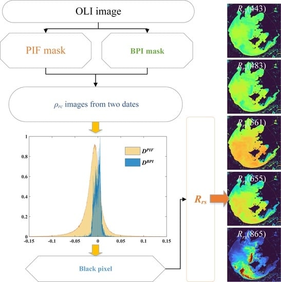
Figure 4.
Processing procedure of the m-ACZI algorithm. Note: These thresholds are for Lake Taihu and may need to be adjusted for other waters [12,17].

Figure 5.
Example of the PIF mask determination. (a) False color image (R: SWIR band, G: NIR band, B: Blue band) with vegetation in green; (b) Construction land and water; and (c) PIF mask over airports near Lake Taihu, China.
Figure 5.
Example of the PIF mask determination. (a) False color image (R: SWIR band, G: NIR band, B: Blue band) with vegetation in green; (b) Construction land and water; and (c) PIF mask over airports near Lake Taihu, China.

Figure 6.
Histogram of DBPI (blue bar) and DPIF (yellow bar) derived by two date images (Dates: 11 May 2017 and 27 May 2017) in Lake Taihu, China.
Figure 6.
Histogram of DBPI (blue bar) and DPIF (yellow bar) derived by two date images (Dates: 11 May 2017 and 27 May 2017) in Lake Taihu, China.

Figure 7.
Comparison of the ACZI and the m-ACZI algorithms for OLI Rrs over Lake Taihu (dates: 11 May 2017, 27 May 2017, and 21 December 2017).
Figure 7.
Comparison of the ACZI and the m-ACZI algorithms for OLI Rrs over Lake Taihu (dates: 11 May 2017, 27 May 2017, and 21 December 2017).

Figure 8.
Frequency of Rrs retrieved using the ACZI (blue) and the m-ACZI (orange) algorithm in Lake Taihu (Dates: 11 May 2017, 27 May 2017, and 21 December 2017).
Figure 8.
Frequency of Rrs retrieved using the ACZI (blue) and the m-ACZI (orange) algorithm in Lake Taihu (Dates: 11 May 2017, 27 May 2017, and 21 December 2017).

Figure 9.
Scatterplots of Rrs derived by the ACZI (a) and the m-ACZI (b) algorithms versus in situ Rrs.
Figure 9.
Scatterplots of Rrs derived by the ACZI (a) and the m-ACZI (b) algorithms versus in situ Rrs.

Figure 10.
Scatterplots of AC-driven Rrs versus in situ Rrs.

Figure 11.
Scatterplots of AC-driven Rrs of different water types versus in situ Rrs. The red points represent water with floating blooms, and the gray points represent un-floating blooms.
Figure 11.
Scatterplots of AC-driven Rrs of different water types versus in situ Rrs. The red points represent water with floating blooms, and the gray points represent un-floating blooms.

Figure 12.
Rayleigh-corrected reflectance (ρrc) in SWIR bands and its ratio (ρrc (1609)/ρrc (2201)) from Lake Taihu on 2 February 2016.
Figure 12.
Rayleigh-corrected reflectance (ρrc) in SWIR bands and its ratio (ρrc (1609)/ρrc (2201)) from Lake Taihu on 2 February 2016.

Figure 13.
Occurrence probability of BPI pixels (a) and its histogram (b) in Lake Taihu (2013–2018).
Figure 13.
Occurrence probability of BPI pixels (a) and its histogram (b) in Lake Taihu (2013–2018).

Figure 14.
Variations in the transmittance (t) in SWIR bands (based on cloudless images from 2013 to 2018, a total of 36 images).
Figure 14.
Variations in the transmittance (t) in SWIR bands (based on cloudless images from 2013 to 2018, a total of 36 images).

Figure 15.
Impact of Δt (means different between t from two date images) on DPIF (1609) (taking Suzhou City (red box) near Lake Taihu as an example). (b) RGB image of Suzhou City (red box in (a)). The average ρsPIF (1609) (c) was driven by ACOLITE based on cloudless images from 2013 to 2018 (total of 36 images). The DPIF is the difference in ρrc (SWIR) for two dates images; the ΔtρsPIF represents the residual surface reflectance caused by Δt in DPIF, and ΔtρsPIF/DPIF is the ratio of ΔtρsPIF to DPIF, which represents the error of DPIF caused by Δt. These two Δt values were the maximum Δt (0.0438) and Δt = 0.0107 (approximate average Δt) from 36 images (2013 to 2018), respectively.


Table 1.
Statistics of the accuracy measures for the ACZI and the m-ACZI algorithms using in situ Rrs measurements. The BLUE number represents the minimal statistical value.
Table 1.
Statistics of the accuracy measures for the ACZI and the m-ACZI algorithms using in situ Rrs measurements. The BLUE number represents the minimal statistical value.
| Method | 443 | 483 | 561 | 655 | 865 | |
|---|---|---|---|---|---|---|
| m-ACZI | RMSE(sr−1) | 0.0063 | 0.0062 | 0.0111 | 0.0082 | 0.0228 |
| sMAPE(%) | 30.71 | 23.01 | 21.41 | 21.27 | 48.31 | |
| Bias(%) | 52.07 | 7.59 | −16.48 | −11.65 | 88.83 | |
| ACZI | RMSE(sr−1) | 0.0070 | 0.0076 | 0.0146 | 0.0102 | 0.0203 |
| sMAPE(%) | 35.88 | 34.07 | 29.16 | 29.10 | 57.48 | |
| Bias(%) | −8.91 | −12.32 | −22.70 | −16.18 | 94.16 |
Table 2.
Statistics of the accuracy measures for the m-ACZI, SeaDAS, DSF, and EXP algorithms using in situ Rrs measurements. The BLUE number represents the minimal statistical value.
Table 2.
Statistics of the accuracy measures for the m-ACZI, SeaDAS, DSF, and EXP algorithms using in situ Rrs measurements. The BLUE number represents the minimal statistical value.
| Method | 443 | 483 | 561 | 655 | 865 | |
|---|---|---|---|---|---|---|
| m-ACZI | RMSE(sr−1) | 0.0063 | 0.0062 | 0.0111 | 0.0082 | 0.0228 |
| sMAPE(%) | 30.71 | 23.01 | 21.41 | 21.27 | 48.31 | |
| Bias(%) | 52.07 | 7.59 | −16.48 | −11.65 | 88.83 | |
| SeaDAS-SWIR | RMSE(sr−1) | 0.0113 | 0.0100 | 0.0108 | 0.0104 | 0.0134 |
| (n = 54) | sMAPE(%) | 45.11 | 32.70 | 20.65 | 27.33 | 76.35 |
| Bias(%) | 33.32 | 13.36 | −1.38 | 4.37 | 126.68 | |
| EXP | RMSE(sr−1) | 0.0060 | 0.0070 | 0.0150 | 0.0105 | 0.0217 |
| sMAPE(%) | 34.12 | 27.76 | 32.79 | 28.29 | 55.56 | |
| Bias(%) | 2.50 | −10.31 | −27.00 | −19.72 | 90.38 | |
| DSF | RMSE(sr−1) | 0.0058 | 0.0061 | 0.0098 | 0.0080 | 0.0244 |
| sMAPE(%) | 32.27 | 24.34 | 17.68 | 21.80 | 63.00 | |
| Bias(%) | 34.22 | 4.94 | −4.46 | 0.01 | 113.55 |
Table 3.
Statistics of the accuracy measures for atmospheric correction algorithms for un-floating blooms using in situ Rrs measurements. The BLUE number represents the minimal statistical value.
Table 3.
Statistics of the accuracy measures for atmospheric correction algorithms for un-floating blooms using in situ Rrs measurements. The BLUE number represents the minimal statistical value.
| Method | 443 | 483 | 561 | 655 | 865 | |
|---|---|---|---|---|---|---|
| m-ACZI | RMSE(sr−1) | 0.0058 | 0.0058 | 0.0087 | 0.0072 | 0.0127 |
| (n = 53) | sMAPE(%) | 25.63 | 20.49 | 18.97 | 17.86 | 48.62 |
| Bias(%) | 21.32 | 3.93 | −14.76 | −10.45 | 91.30 | |
| ACZI | RMSE(sr−1) | 0.0071 | 0.0073 | 0.0109 | 0.0085 | 0.0112 |
| (n = 53) | sMAPE(%) | 31.77 | 25.94 | 23.13 | 22.59 | 59.54 |
| Bias(%) | −6.01 | −6.81 | −18.20 | −10.54 | 102.18 | |
| SeaDAS-SWIR | RMSE(sr−1) | 0.0113 | 0.0101 | 0.0107 | 0.0103 | 0.0123 |
| (n = 48) | sMAPE(%) | 44.17 | 31.74 | 20.02 | 26.57 | 74.39 |
| Bias(%) | 30.91 | 11.20 | −2.26 | 2.61 | 119.49 | |
| EXP | RMSE(sr−1) | 0.0058 | 0.0068 | 0.0126 | 0.0093 | 0.0123 |
| (n = 53) | sMAPE(%) | 26.63 | 24.18 | 30.28 | 24.10 | 55.98 |
| Bias(%) | −3.30 | −10.77 | −25.36 | −17.42 | 93.74 | |
| DSF | RMSE(sr−1) | 0.0055 | 0.0058 | 0.0075 | 0.0068 | 0.0144 |
| (n = 53) | sMAPE(%) | 26.92 | 21.81 | 15.16 | 19.31 | 65.51 |
| Bias(%) | 8.72 | 3.16 | −1.85 | 1.95 | 117.79 |
Table 4.
Statistics of the accuracy measures for atmospheric correction algorithms for floating bloom using in situ Rrs measurements. The BLUE number represents the minimal statistical value.
Table 4.
Statistics of the accuracy measures for atmospheric correction algorithms for floating bloom using in situ Rrs measurements. The BLUE number represents the minimal statistical value.
| Method | 443 | 483 | 561 | 655 | 865 | |
|---|---|---|---|---|---|---|
| m-ACZI | RMSE(sr−1) | 0.0078 | 0.0072 | 0.0162 | 0.0107 | 0.0396 |
| (n = 18) | sMAPE(%) | 45.68 | 30.42 | 28.61 | 31.29 | 47.40 |
| Bias(%) | 142.60 | 18.39 | −21.53 | −15.18 | 81.53 | |
| ACZI | RMSE(sr−1) | 0.0067 | 0.0086 | 0.0222 | 0.0140 | 0.0355 |
| (n = 18) | sMAPE(%) | 51.47 | 58.00 | 46.92 | 48.25 | 51.41 |
| Bias(%) | −19.90 | −28.52 | −35.93 | −32.81 | 70.54 | |
| SeaDAS-SWIR | RMSE(sr−1) | 0.0111 | 0.0097 | 0.0115 | 0.0110 | 0.0204 |
| (n = 6) | sMAPE(%) | 52.71 | 40.43 | 25.69 | 33.33 | 92.05 |
| Bias(%) | 52.55 | 30.56 | 5.67 | 18.46 | 184.26 | |
| EXP | RMSE(sr−1) | 0.0067 | 0.0075 | 0.0205 | 0.0134 | 0.0376 |
| (n = 18) | sMAPE(%) | 56.19 | 38.30 | 40.20 | 40.63 | 54.32 |
| Bias(%) | 19.58 | −8.93 | −31.81 | −26.47 | 80.47 | |
| DSF | RMSE(sr−1) | 0.0067 | 0.0070 | 0.0147 | 0.0107 | 0.0416 |
| (n = 18) | sMAPE(%) | 48.00 | 31.78 | 25.10 | 29.13 | 55.60 |
| Bias(%) | 109.31 | 10.17 | −12.16 | −5.71 | 101.07 |
Disclaimer/Publisher’s Note: The statements, opinions and data contained in all publications are solely those of the individual author(s) and contributor(s) and not of MDPI and/or the editor(s). MDPI and/or the editor(s) disclaim responsibility for any injury to people or property resulting from any ideas, methods, instructions or products referred to in the content. |
© 2023 by the authors. Licensee MDPI, Basel, Switzerland. This article is an open access article distributed under the terms and conditions of the Creative Commons Attribution (CC BY) license (https://creativecommons.org/licenses/by/4.0/).
Share and Cite
MDPI and ACS Style
Wang, D.; Xiang, X.; Ma, R.; Guo, Y.; Zhu, W.; Wu, Z. A Novel Atmospheric Correction for Turbid Water Remote Sensing. Remote Sens. 2023, 15, 2091. https://0-doi-org.brum.beds.ac.uk/10.3390/rs15082091
AMA Style
Wang D, Xiang X, Ma R, Guo Y, Zhu W, Wu Z. A Novel Atmospheric Correction for Turbid Water Remote Sensing. Remote Sensing. 2023; 15(8):2091. https://0-doi-org.brum.beds.ac.uk/10.3390/rs15082091
Chicago/Turabian StyleWang, Dian, Xiangyu Xiang, Ronghua Ma, Yongqin Guo, Wangyuan Zhu, and Zhihao Wu. 2023. "A Novel Atmospheric Correction for Turbid Water Remote Sensing" Remote Sensing 15, no. 8: 2091. https://0-doi-org.brum.beds.ac.uk/10.3390/rs15082091
Note that from the first issue of 2016, this journal uses article numbers instead of page numbers. See further details here.