Mapping Growing Stem Volume Using Dual-Polarization GaoFen-3 SAR Images in Evergreen Coniferous Forests

Abstract

Unaffected by cloud cover and solar illumination, synthetic aperture radar (SAR) images have great capability to map forest growing stem volume (GSV) in complex biophysical environments. Up to now, c-band dual-polarization Gaofen-3 (GF-3) SAR images, acquired by the first Chinese civilian satellite equipped with multi-polarized modes, are rarely applied in mapping forest GSV. To evaluate the capability of dual-polarization GF-3 SAR images in mapping forest GSV, several proposed derived features were initially extracted by mathematical operations and applied to obtain optimal feature sets by different feature sorting methods and feature selection methods. Then, the maps of GSV in an evergreen coniferous forest were inverted by various machine learning algorithms and stacking ensemble learning methods with different strategies. The results implied that backscattering coefficients and partially proposed derived features showed high sensitivity to the forest GSV, and the saturation phenomenon also obviously occurred once the forest GSV was larger than 300 m³/ha. Furthermore, the results showed that the accuracy of the mapped GSV was significantly improved using the stacking ensemble learning methods. Using various optimal feature sets and base models (MLR, KNN, SVM, and RF), the rRMSE values mainly ranged from 30% to 40%. After using the stacking ensemble learning methods, the values of rRMSE ranged from 16.71% to 20.51%. This confirmed that dual-polarization GF-3 images have great potential to map forest GSV in evergreen coniferous forests.

1. Introduction

Forest growing stem volume (GSV) is widely applied to evaluate forest resources and the potential carbon sink of forest ecosystems [1,2,3,4,5]. In recent years, due to the complex ecological conditions of forests and the limitations of field investigations, remote sensing technology has become an important method for forest mapping and dynamic monitoring [6,7,8]. However, because of cloud cover and spectral saturation phenomena, the optical remote sensing images are limited to accurately mapping forest GSV in mountainous areas [9,10,11]. Unaffected by cloud cover and solar illumination, synthetic aperture radar (SAR) images have great capability to penetrate the canopies by emitting radiation to detect and measure branches and trunks [11,12].

Recently, satellite-based SAR sensors with various bands (X, C, and L band) and various polarization (single, dual, and quad) SAR images have been widely applied in mapping forest parameters, such as TerraSAR-X, Rardarsat-2, ALSO-2 PALSAR, and Sentinel-1 [7,13]. Furthermore, previous results have shown that changes in wavelength and types of polarization modes resulted in differences in both analytical workflows and the achieved estimation performances [9,14]. Meanwhile, the penetration of microwaves with different bands also affected the accuracy of mapping forest GSV, especially for coniferous forests with high forest GSV [15,16,17,18,19]. In a previous study, it also has been proven that features obtained from cross-polarization (HV) were more sensitive with forest GSV than those from co-polarization (HH or VV) for the same band [20,21,22]. Furthermore, multi-bands and multi-temporal SAR images were also applied to improve the accuracy of mapping forest GSV, and these combination methods were superior in prediction [14,20,23], yet the saturation still happened at the high GSV levels, especially for mature and over-mature coniferous forests.

To delay saturation levels in mapping forest parameters, it has been confirmed that quad polarization SAR images performed better than single and dual-polarization SAR images [12]. However, among the available SAR images, the number of images acquired with single and dual-polarization modes was much larger than that acquired with quad polarization modes. Therefore, dual-polarization SAR images with C and L bands are still a compromise option for forest applications in large areas at present. In addition, a C-band Gaofen-3 (GF-3) SAR sensor, launched on 10 August 2016, is the first Chinese civilian satellite to be equipped with multi-polarized modes [11,24,25]. Recently, most applications with GF-3 SAR images mainly focused on vegetation classification and sea applications [11,24,25,26,27]. However, previous studies rarely used GF-3 images with various polarization modes for quantitative estimating of forest parameters. Therefore, it is meaningful to evaluate the potentiality of GF-3 images for mapping forest GSV, especially for dual-polarization GF-3 images in evergreen coniferous forests.

Furthermore, extracting enough features from dual-polarization SAR images is one of the key steps for analyzing the relationships between SAR images and forest GSV [11,24,25,26,27,28,29,30]. Limiting polarization models and backscattering coefficients with different polarizations and features derived from a non-coherent covariance matrix are commonly extracted from dual-polarization SAR images [23,31]. In a previous study, the backscattering coefficients of dual SAR images have been proven to be appropriate for estimating forest GSV. To overcome the lack of features extracted from dual-polarization images, textural features derived by a gray level concurrence matrix (GLCM) are often employed to obtain intensity images [32,33]. So, extracting enough features from dual-polarization SAR images is helpful to improve the accuracy of mapping forest GSV.

Moreover, the accuracy of mapping forest GSV is severely dependent on the optimal feature sets and employed models. The optimal feature set is determined by feature evaluating criteria and feature selection methods [8,11,34]. Until now, the feature evaluation criteria were mainly based on the linear or nonlinear relationships between features and GSV, such as importance derived from the random forest algorithm (RF), distance correlation coefficient (DC), maximal information coefficient (MIC), and Pearson correlation coefficient. Different feature evaluation criteria obtain different orders with alternative features. Furthermore, the feature selection methods can be broadly classified into three categories: filters, wrappers, and embedded [6,8]. Therefore, various optimal feature sets can be obtained from various combinations of feature evaluation criteria and feature selection methods. However, it is a thorny issue for selecting the appropriate feature evaluation criteria and feature selection methods for mapping forest GSV. Additionally, the accuracy of the mapped GSV is also determined by employed models, such as parameter models and non-parameters [23,35,36]. Up to now, many models, including the multiple linear regression model (MLR), RF, K-nearest neighbor (K-NN), support vector machine (SVM), and artificial neural network mode (ANN) [37], were also widely used to map forest GSV, and the gaps between inverted forest GSV with different models are striking. Thereby, to overcome the gaps induced by optimal feature sets and employed models, ensemble learning algorithms are an effective way to reduce the variations [38].

The objective of this study is to evaluate the capability of C-band dual-polarization GF-3 SAR images for mapping GSV in evergreen coniferous forests. After image pre-processing, several proposed derived features were initially extracted by mathematical operations. Then, two feature evaluation criteria and wrapped feature selection methods with four models were proposed to obtain various optimal feature sets. Finally, various strategies of stacking ensemble approach with two meta-models were proposed to estimate forest GSV based on predicted results from four base models, and the gaps between mapped forest GSV by different strategies were evaluated. Meanwhile, the capability of C-band dual-polarization GF-3 SAR images was also evaluated in terms of the sensitivity between features and GSV and the accuracy of mapped forest GSV.

2. Study Area and Data

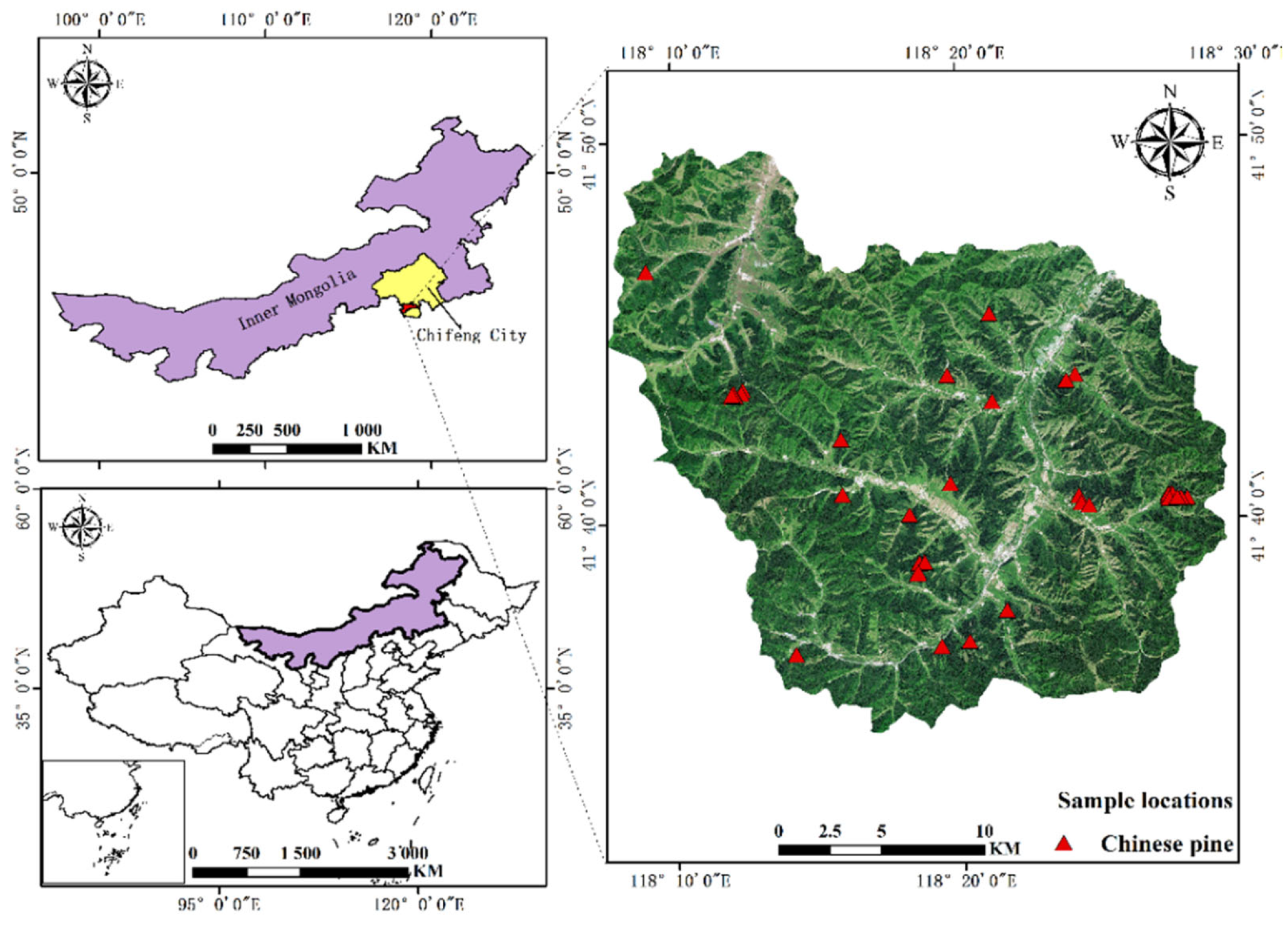
2.1. Study Area

The study area focused on the Wangyedian Experimental Forest Farm (118°0″ E~118°3″ E, 41°2″ N~41°3″ N) located in the southwest of Harqin Banner, Chifeng City, Inner Mongolia, China (Figure 1). The study area is a branch of Qilaotu Mountain at the northern foot of the Yanshan Mountains, with an elevation varying from 600 m to 1890 m. Influenced by the temperate monsoon climate, the average annual temperature of the study area is 4.2 °C, and annual precipitation ranges from 400 mm to 600 mm. The forest area was up to 23,300 ha and the percentage of forest cover was near 93% by the end of 2016, with a total stem volume of 1.41 million m³, and the annual growth of GSV is forty-eight thousand m³. The main plantation tree species include larch (Larix principis-rupprechtii and Larix olgensis) and Chinese pine (Pinus tabuliformis).

2.2. Ground Data and Procession

Based on the age group, terrain, and spatial distribution of planted Chinese pines, 42 ground samples with a size of 25 m × 25 m were set in the study area (Figure 1). The ground measurements were conducted from 20 September to 15 October 2017. For each sample, the corners and central points were accurately measured by a global positioning system (GPS). Then, several parameters of each tree with a diameter at breast height (DBH) larger than 5 cm were measured, such as height, DBH, and the size of the canopy. The timber volume of each tree was calculated using the equations related to the measured height and DBH, provided by the Wangyedian forest farm [6]:

$$V=0.013464-0.001967\times D+0.000089\times D^2+0.000628\times D\times H+0.000032\times H\times D^2-0.003173\times H$$

(1)

where V is the timber volume of each tree, and H and D are the height and DBH of each tree, respectively. The GSV of the ground sample was the sum of all the tree timber volume within the plot. In this study, the GSV of all measured samples ranges from 91.97 m³/ha to 514.96 m³/ha, and the average GSV and Std are 254.49 m³/ha and 113.08 m³/ha, respectively.

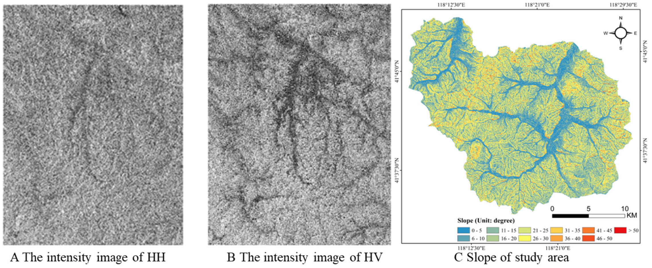
2.3. GF-3 Dual-Polarimetric SAR Images and DEM

The GF-3 satellite, launched in 2016, is the highest resolution C-band (1 m) and multi-polarization SAR satellite in the world. It has twelve imaging modes, which can be freely switched into multiple imaging modes such as spot beam, strip, scan, wave, global observation, and high and low incidence angle [26,39]. In this study, dual-polarization GF-3 SAR images (HH, HV) with a range resolution of 2.25 m and an azimuthal resolution of 3.12 m were acquired on 18 March 2017. The gray intensity images of HH and HV are shown in Figure 2A,B. Additionally, for geocoding the SAR images, an external digital elevation model (DEM) with a resolution of 12.5 m, generated by interferometric synthetic aperture radar (InSAR) technology (Figure 2C), was downloaded from NASA-EARTHDATA (https://search.asf.alaska.edu/, accessed on 18 March 2020).

2.4. Image Pre-Processing

Before extracting features from images, there are several steps to pre-process dual-polarization GF-3 SAR images for reducing noise and radiometric errors, including radiometric calibration, adaptive filtering, terrain correction, and geocoding [25,39]. Firstly, radiometric calibration was performed to obtain the quantitative backscattering coefficient, and then, the refined Lee filter (7 × 7) was adopted to retrieve homogeneous pixels for reducing the errors caused by the speckle noise [12,22]. Secondly, the errors induced by terrain slope were corrected by terrain radiometric correction with external DEM. After that, the dual-polarization SAR images were resampled to generate geocoding products with a size of 5 m × 5 m using external DEM.

3. Methods

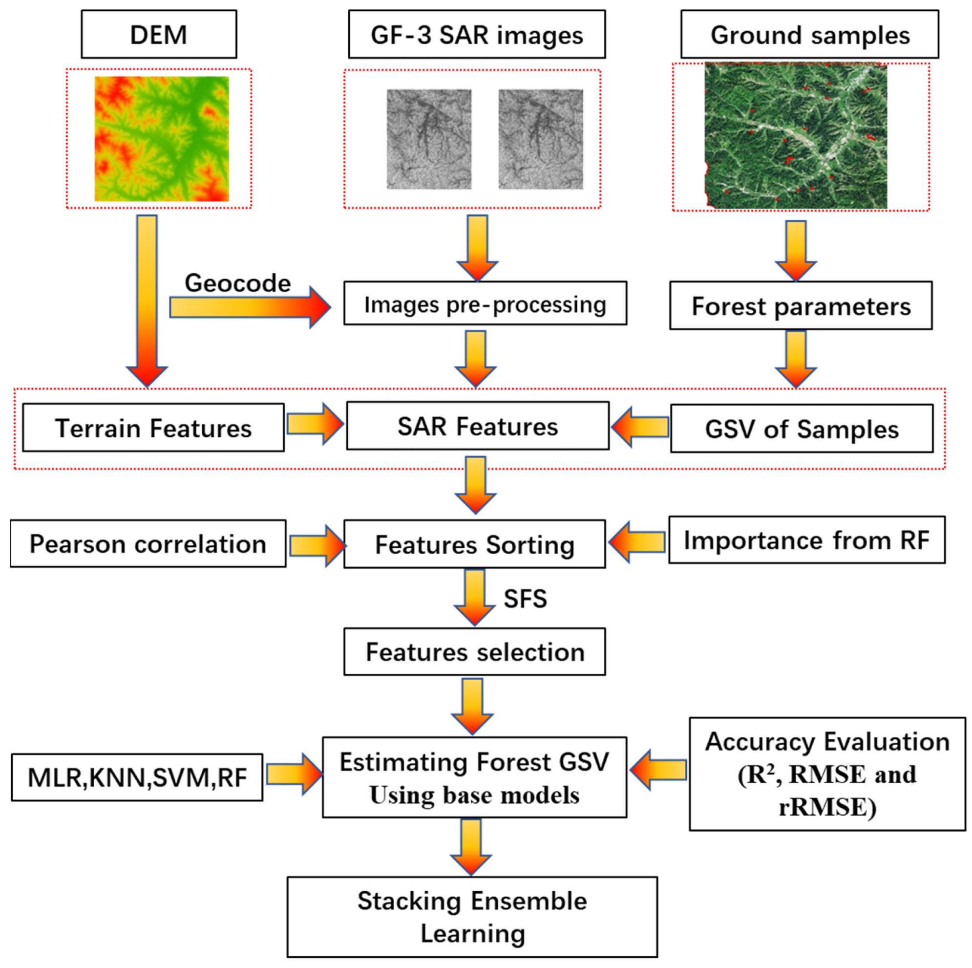
3.1. Research Framework

In this study, dual-polarization GF-3 SAR images were employed to extract backscattering coefficients, derived features, and textural features. Combined with ground-measured samples and external DEM, Pearson correlation and importance derived from RF between features and forest GSV were selected as feature sorting criteria. After feature sorting, various optimal feature sets were obtained by sequential forward selection (SFS) with various feature selection methods combined with different machine learning models (SFS-MLR, SFS-KNN, SFS-SVM, and SFS-RF). Then, various predicted results were obtained by four base models (MLR, KNN, SVM, and RF) for every obtained optimal feature set, respectively. Finally, stacking ensemble learning approaches with different strategies were constructed based on different predicted forest GSV within feature sorting methods and feature selection methods (Figure 3).

3.2. Feature Extraction from GF-3 SAR Images

Normally, it is very important to extract enough alternative features from dual-polarization GF-3 SAR images. In this study, various types of features were initially extracted from dual-polarization GF-3 SAR images after pre-precession. Different from quad-polarization data, just two backscattering coefficients (σ_HH and σ_HV) can be extracted from dual-polarization SAR images. For expanding the number of alternative features, sixteen derived features related to backscattering coefficients were proposed by mathematical operations in this study (

Table 1. The list of alternative features extracted from dual-polarization GF-3 SAR images.

Number	Feature	Note	Number	Feature	Note	Number	Feature	Note
1	SHH	$\sqrt{a^2+b^2}$	11	C7	σHV/(σHH + σHV)	21	Mean	5 × 5, 7 × 7, 9 × 9
2	SHV	$\sqrt{a^2+b^2}$	12	C8	σHH 2	22	Variance	5 × 5, 7 × 7, 9 × 9
3	σHH	dB	13	C9	σHV 2	23	Homogeneity	5 × 5, 7 × 7, 9 × 9
4	σHV	dB	14	C10	(C1)2	24	Contrast	5 × 5, 7 × 7, 9 × 9
5	C1	σHH + σHV	15	C11	(C2)2	25	Dissimilarity	5 × 5, 7 × 7, 9 × 9
6	C2	σHH − σHV	16	C12	(C3)2	26	Entropy	5 × 5, 7 × 7, 9 × 9
7	C3	σHH/σHV	17	C13	(C4)2	27	Second Moment	5 × 5, 7 × 7, 9 × 9
8	C4	σHH × σHH	18	C14	(C5)2	28	Correlation	5 × 5, 7 × 7, 9 × 9
9	C5	(σHH − σHV)/(σHH + σHV)	19	C15	(C6)2
10	C6	σHH/(σHH + σHV)	20	C16	(C7)2

Note: a and b are the real and imaginary components of SLC data, S_HH and S_HV are the intensity of HH and HV polarization with a linear form, σ_HH and σ_HV are backscattering coefficients of HH and HV polarization, C1-C16 are derived features related to backscattering coefficients of σ_HH and σ_HV, 5 × 5, 7 × 7, and 9 × 9 indicate the window size of obtaining textural features by GLCM.

).

Furthermore, textural information was also extracted from each polarized intensity image (σ_HH and σ_HV) based on second-order statistics using the gray level concurrence matrix (GLCM). Eight textural features of each image with various window sizes (ranging from five to nine), including mean, variance, homogeneity, contrast, dissimilarity, entropy, second moment, and correlation, were applied for mapping GSV in planted Chinese pine forests. Additionally, four terrain features were also extracted from external DEM.

3.3. The Approaches of Feature Selection

For mapping forest GSV, feature selection has two main objectives, which are to maximize the regression performance (minimize the regression errors) and to minimize the number of features. Optimizing the feature set is required before feeding it into machine learning algorithms for improving the regression process and making it cost- and time-efficient. Normally, the number of the optimal feature set and the accuracy of estimated GSV are highly related to the strategies of feature selection. Commonly, sequential forward selection (SFS) and sequential backward selection (SBS) are mainly used in wrapped feature selection methods [40]. In this study, the strategy of optimizing the feature set includes two steps, feature sorting and feature selection with SFS.

Firstly, these extracted alternative features should be sorted by feature evaluation criteria. Normally, feature evaluation criteria are used to quantitatively express the relationship between features and forest GSV. Recently, several criteria are widely applied to express the relationships, such as the Pearson correlation coefficient, DC, MIC, and importance derived from RF [8,41]. In this study, the rank of alternative features is sorted by the Pearson correlation coefficient and importance is derived from RF.

Then, the SFS method was applied to obtain optimal feature sets for two sorted features with several machine learning algorithms (MLR, KNN, SVM, and RF). Ultimately, four optimal feature sets were formed for each feature evaluation criterion. In addition, to describe the regression performance, the root-mean-square error (RMSE) derived from the leave-one-out cross-validation method (LOOCV) was employed to evaluate the capability of feature selection methods, and the optimal feature set was finally determined by the smallest RMSE value [12]. In the next procession, the forest GSV would be mapped using these derived optimal feature sets.

3.4. Stacking Ensemble Learning and Strategies

Recently, widely used machine learning algorithms have significant advantages in solving complex, non-linear, and highly uncertain problems. In this study, four machine learning algorithms (MLR, KNN, SVM, and RF) were employed to estimate forest GSV. Normally, the accuracy of estimated forest GSV is highly related to the selected feature set and employed models. To reduce this dependence, ensemble learning with different strategies was constructed using various feature selection methods and base models.

In this study, within each feature sorting method (Pearson correlation and importance), four feature selection methods (SFS-MLR, SFS-KNN, SF-SVM, and SFS-RF) were applied to obtain optimal feature sets, and then each optimal feature set was used to estimate forest GSV by four base models (MLR, KNN, SVM, and RF), respectively. To reduce the influence of feature selection methods and estimation models, stacking ensemble learning with different strategies was applied to derive the final predicted forest GSV. In this study, two meta-learnings (MLR and SVM with a linear kernel) were applied to construct the stacking ensemble learning algorithms. Considering the difference between feature selection methods and feature sorting methods, stacking ensemble learning with different strategies were listed in

Table 2. The list of stacking ensemble learning with different strategies.

Serial Number	FS Methods (Feature Sorting-Models)	Base Model	Number of Predictions	Meta-Learning for Stacking Ensemble
1	Pearson-MLR	MLR, KNN, SVM, and RF	4	MLR and SVM
2	Pearson-KNN	MLR, KNN, SVM, and RF	4	MLR and SVM
3	Pearson-SVM	MLR, KNN, SVM, and RF	4	MLR and SVM
4	Pearson-RF	MLR, KNN, SVM, and RF	4	MLR and SVM
5	Importance-MLR	MLR, KNN, SVM, and RF	4	MLR and SVM
6	Importance -KNN	MLR, KNN, SVM, and RF	4	MLR and SVM
7	Importance -SVM	MLR, KNN, SVM, and RF	4	MLR and SVM
8	Importance -RF	MLR, KNN, SVM, and RF	4	MLR and SVM
9	Pearson sorting	MLR, KNN, SVM, and RF	16	MLR and SVM
10	Importance sorting	MLR, KNN, SVM, and RF	16	MLR and SVM

.

For evaluating the accuracy of mapped forest GSV, the LOOCV method was applied to obtain the predicted GSV of each sample. Then, the root-mean-square error (RMSE), the relative-mean-square error (rRMSE), and the coefficient of determination (R²) between the predicted and measured GSV were calculated to evaluate the models. The calculation formulas are as follows:

$$R^2=1-\frac{{\sum }_{i=1}^{\mathrm{n}}{\left({\mathrm{y}}_{\mathrm{i}}-{ \widehat{\mathrm{y}}}_{\mathrm{i}}\right)}^2}{{\sum }_{i=1}^{\mathrm{n}}{\left({\mathrm{y}}_{\mathrm{i}}-\overline{\mathrm{y}}\right)}^2}$$

(2)

$$RMSE=\sqrt{\frac{{\sum }_{i=1}^{\mathrm{n}}{\left({\mathrm{y}}_{\mathrm{i}}-{ \widehat{\mathrm{y}}}_{\mathrm{i}}\right)}^2}{n}}$$

(3)

$$rRMSE=\frac{RMSE}{\overline{y}}\times 100\%$$

(4)

where ${\mathrm{y}}_{\mathrm{i}}$ and ${ \widehat{\mathrm{y}}}_{\mathrm{i}}$ are the measured and predicted GSV of sample $i$, $\overline{\mathrm{y}}$ is the average of measured GSV, and $i$ is the number of samples.

4. Results

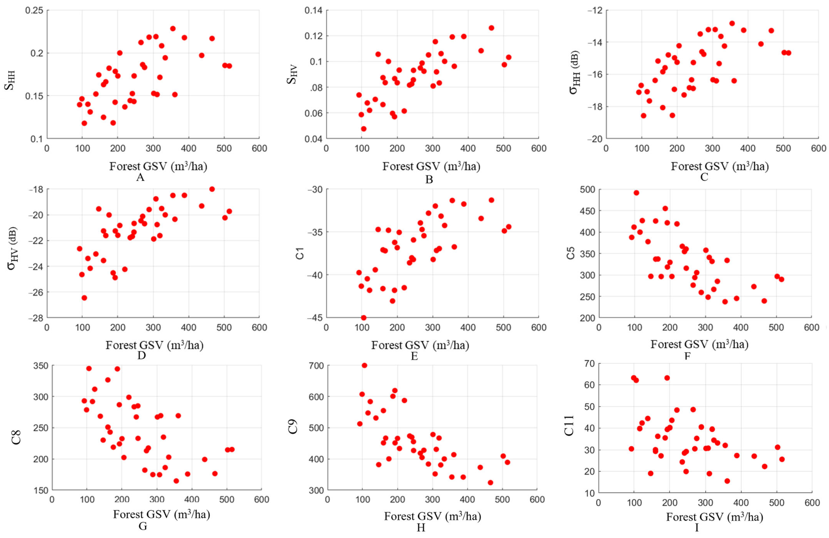
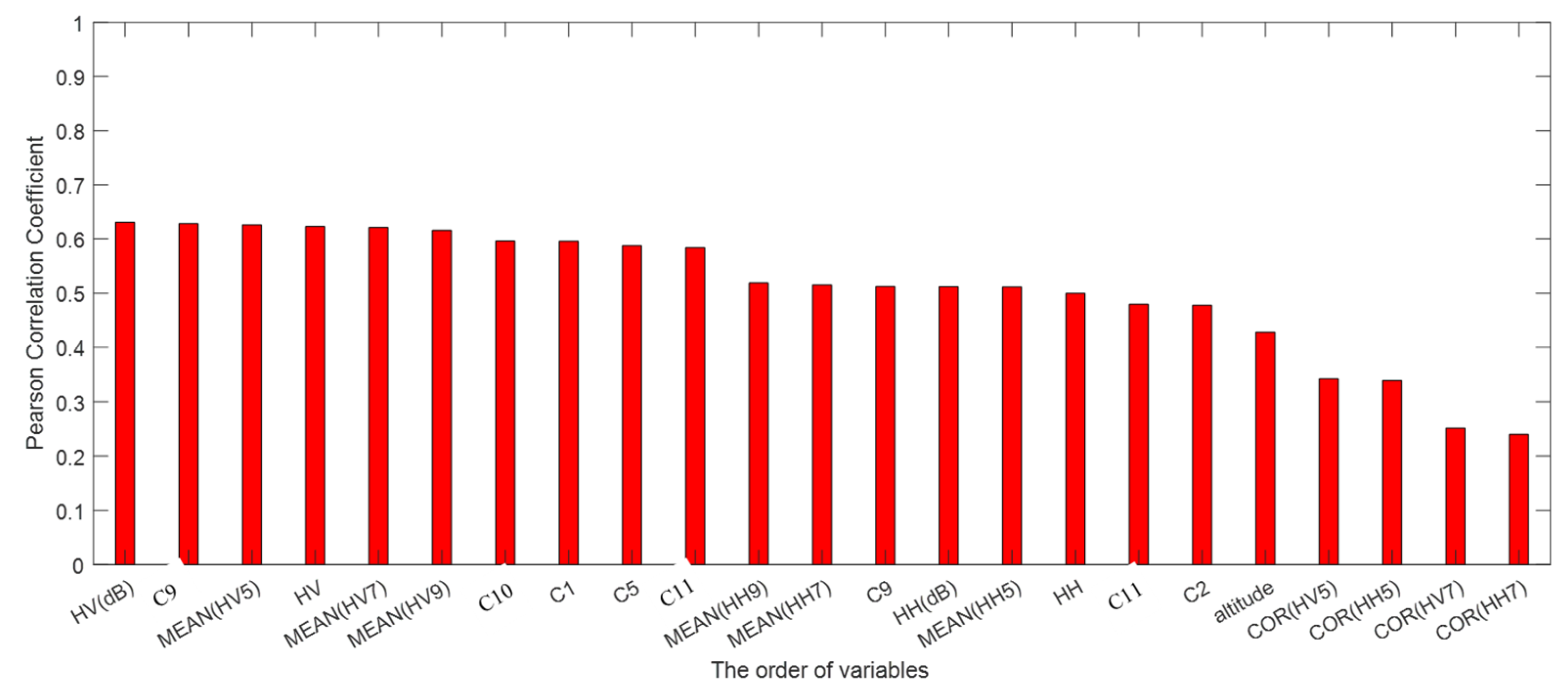
4.1. The Sensitivity between Extracted Features and Forest GSV

In this study, there were seventy-two alternative features extracted from dual-polarization GF-3 SAR images and external DEM. To illustrate the sensitivity between alternative features and forest GSV, scatterplots between partial features and GSV were shown in Figure 4. The results demonstrated that there was a good correlation between variables and forest GSV. Furthermore, the saturation phenomenon obviously occurred once the forest GSV was larger than 300 m³/ha.

Recently, Pearson correlation and importance derived from RF are common criteria to evaluate the sensitivity between the alternative features and forest GSV. In this study, feature sorting methods (Pearson correlation and the importance of RF) were employed to obtain sorted features in descending order. The correlations between alternative features and forest GSV ranged from 0 to 0.63, and the top five features were σ_HV with different forms, mean extracted from HV images with diverse sizes, and C9 (Figure 5). Meanwhile, the results of sorting features using the importance of RF were inconsistent with using Pearson correlation, and the top five features were C9, C5, mean (HV9), σ_HV, and C1. It was found that the orders of features depended on evaluating criteria, and the results of feature selection were naturally different. Therefore, the sorted features were employed to obtain optimal feature sets with different feature selection methods in the next steps.

4.2. The Results of Feature Selection

After feature sorting with two evaluating criteria, sequential forward selection (SFS) with various models (MLR, KNN, SVM, and RF) were applied to obtain the optimal feature set, respectively. For each feature sorting method, there were four optimal feature sets. The number of features in each optimal feature set were related to the feature sorting methods and feature selection methods (

Table 3. Information of optimal feature sets derived from various feature sorting methods and various feature selection methods.

Feature Sorting	FS Methods	Number of Features	The Optimal Feature Set
Pearson correlation	MLR	3	σHV, CORHH5, CORHV5
	KNN	6	σHV σHV (dB), C9, C10, MeanHV9, Aspect
	SVM	2	σHV, σHV (dB)
	RF	12	σHV σHV (dB), σHH (dB) C8, C9, C14, MeanHV5, MeanHV7, MeanHH7, CORHH7VARIHH9, DISMHV7
Importance of RF	MLR	3	C9, σHV, CORHV5
	KNN	3	C9, C5, C10
	SVM	2	C9, σHV
	RF	12	C9, σHV, σHH, altitude, CORHV5, HOMOHH5, SMHH5, DISMHH5, DISMHV5, CORHH7, CONTHV5, VARIHH9

).

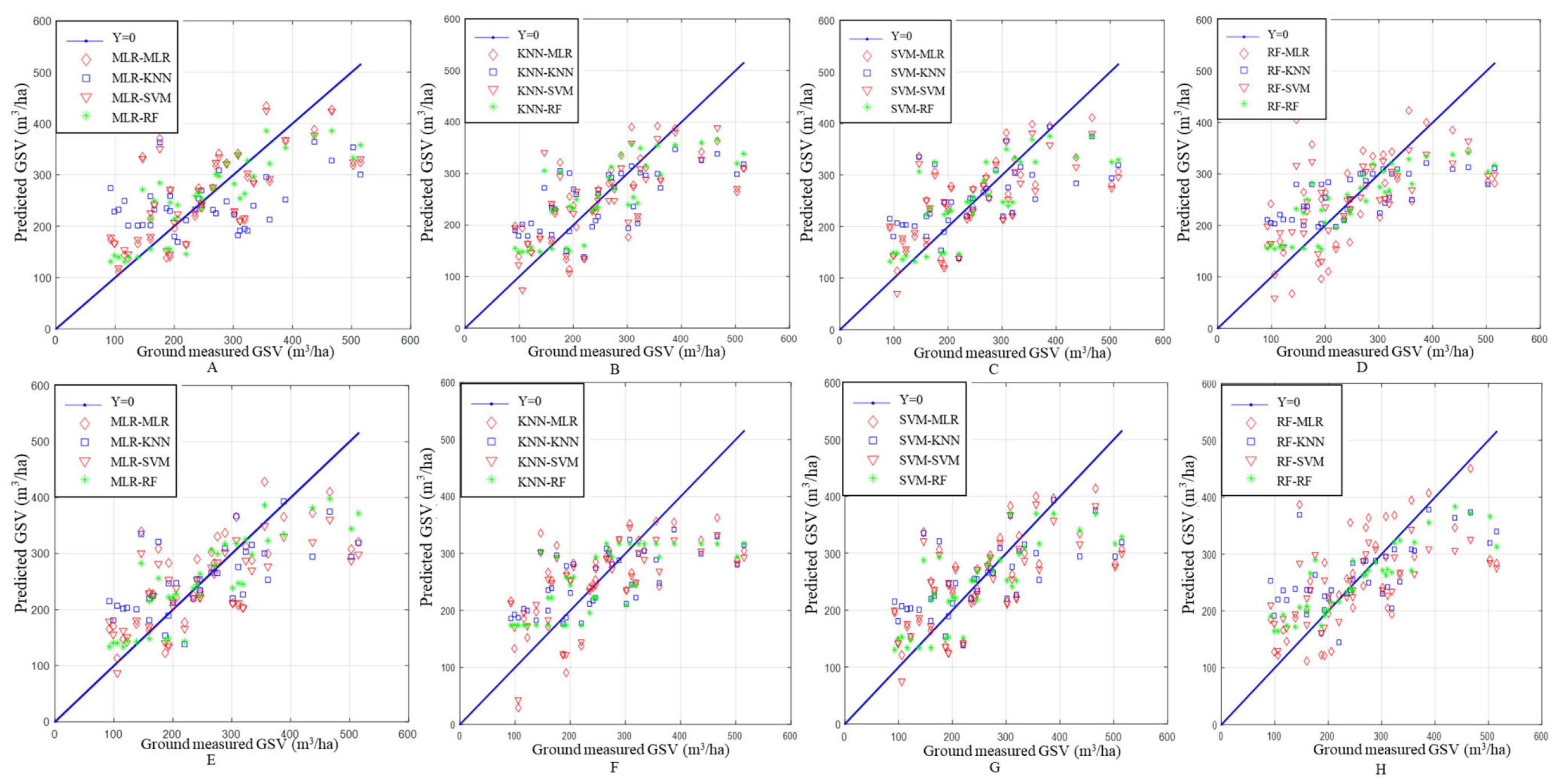
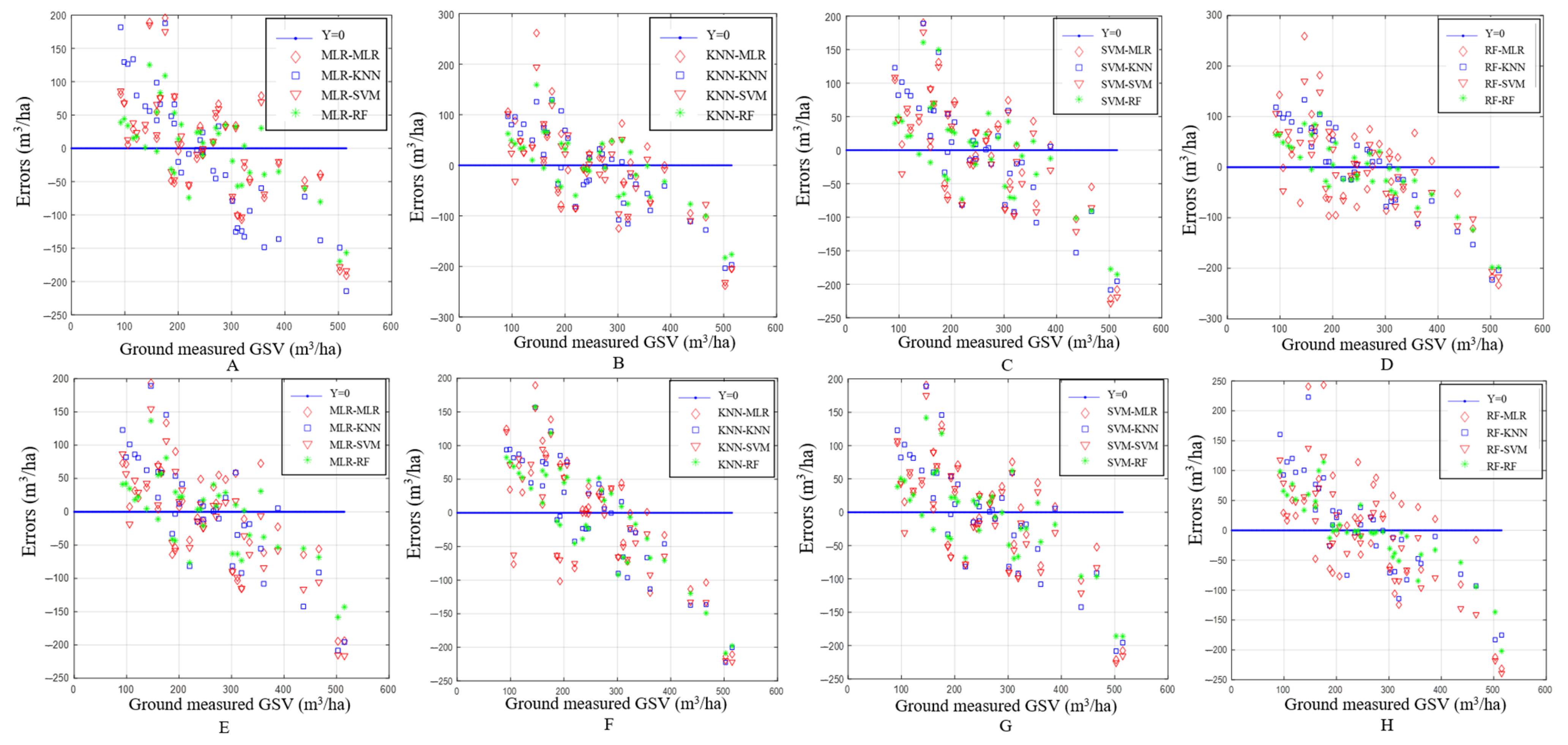
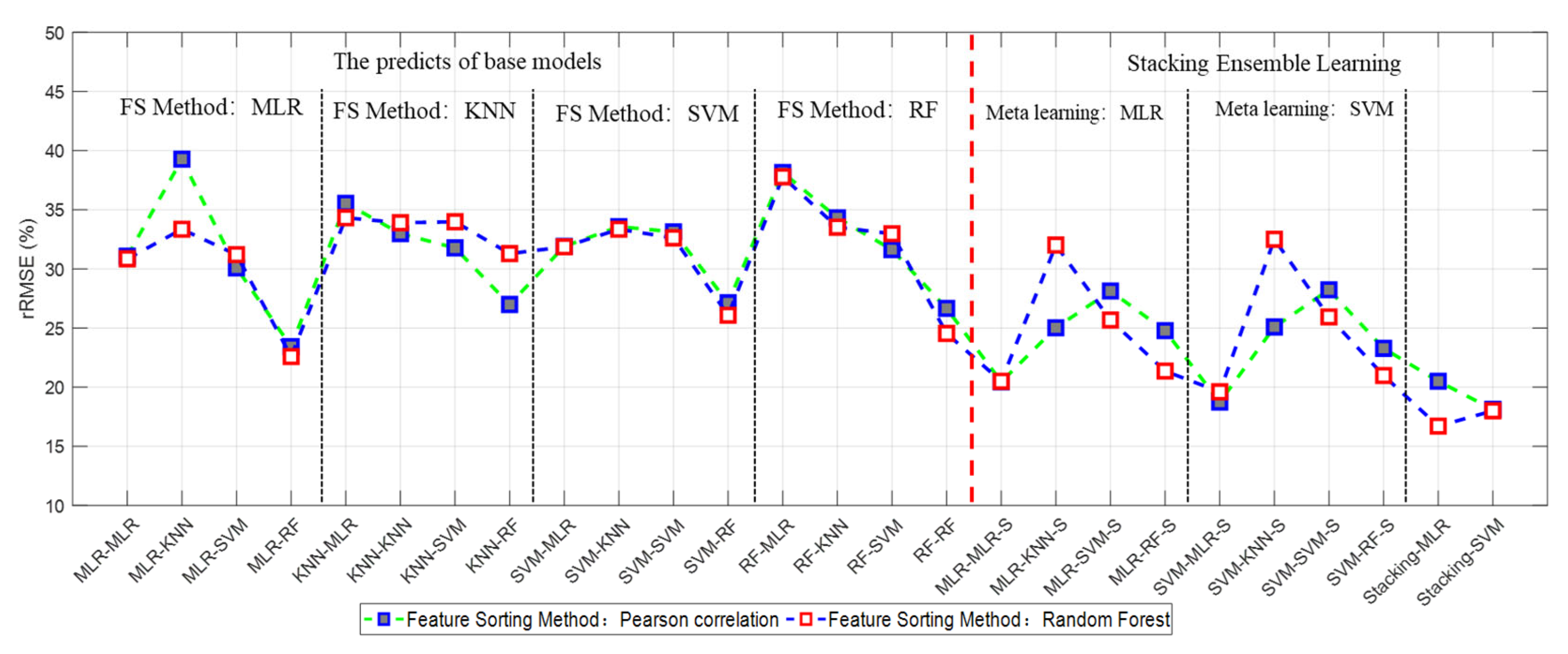
4.3. Estimated GSV Using Base Models

After obtaining the optimal feature sets, four base models (MLR, KNN, SVM, and RF) were applied to estimate the forest GSV. Three accuracy indices (R², RMSE, and rRMSE) were employed to evaluate the estimated results (

Table 4. The results of accuracy indices derived from base models using optimal feature sets.

The Method of FS	Base Model	Sorting Method Pearson Correlation			Sorting Method Importance of RF
		RMSE (m3/ha)	rRMSE (%)	R2	RMSE (m3/ha)	rRMSE (%)	R2
MLR	MLR	79.09	31.08	0.58	78.53	30.86	0.57
	KNN	99.94	39.28	0.21	84.88	33.36	0.30
	SVM	76.57	30.09	0.54	79.42	31.21	0.37
	RF	59.62	23.43	0.51	57.50	22.60	0.53
KNN	MLR	90.46	35.55	0.54	87.35	34.33	0.48
	KNN	83.94	32.99	0.27	86.28	33.91	0.21
	SVM	80.86	31.78	0.50	86.48	33.99	0.36
	RF	68.70	27.00	0.45	79.66	31.30	0.27
SVM	MLR	81.19	31.91	0.51	81.11	31.87	0.51
	KNN	85.46	33.58	0.29	84.88	33.36	0.30
	SVM	84.34	33.14	0.45	83.02	32.63	0.45
	RF	69.07	27.14	0.51	66.40	26.09	0.47
RF	MLR	97.11	38.16	0.61	96.17	37.79	0.62
	KNN	87.33	34.32	0.14	85.31	33.53	0.27
	SVM	80.49	31.63	0.40	83.91	32.98	0.24
	RF	67.86	26.67	0.32	62.48	24.55	0.31

). For the same feature sorting method, the results illustrated that the accuracy of the estimated forest GSV was related to the feature selection methods and base models. Specifically, using the optimal feature set derived from the feature selection method with MLR, the rRMSE ranged from 23.43% to 39.28% for the sorting method with Pearson correlation, and from 22.60% to 33.36% for the sorting method with the importance of RF, respectively. Furthermore, in all feature sorting methods, the best and the worst results of the base model were obtained by RF (rRMSE is 23.43% for the sorting method with Pearson correlation and 22.60% for the sorting method with importance) and KNN (rRMSE is 39.28% for the sorting method with Pearson correlation and 33.36% for the sorting method with importance).

Moreover, for various feature sorting and feature selection methods, the rRMSE derived from MLR, KNN, and SVM ranged from 30% to 40%, and the values derived from RF ranged from 20% to 30%. The RF model has higher accuracy of estimated forest GSV because the result is obtained from the ensemble learning with multiple decision trees. This inferred that the accuracy of estimated forest GSV was rather related to the capability of base models and feature selection methods. However, it is a very tricky problem to evaluate which feature selection method or model is optimal for mapping forest GSV.

Furthermore, the scatterplots between ground-measured and predicted GSV by various feature sorting methods, FS methods, and base models were shown in Figure 6. The overestimated and underestimated samples often occurred for most predicted forest GSV using various base models, and these results obtained by MLR and KNN were more obvious than those by RF and SVM. Because of the saturation phenomenon, it is still difficult to obtain accurate estimation results using a single base model when the forest GSV is larger than 400 m³/ha.

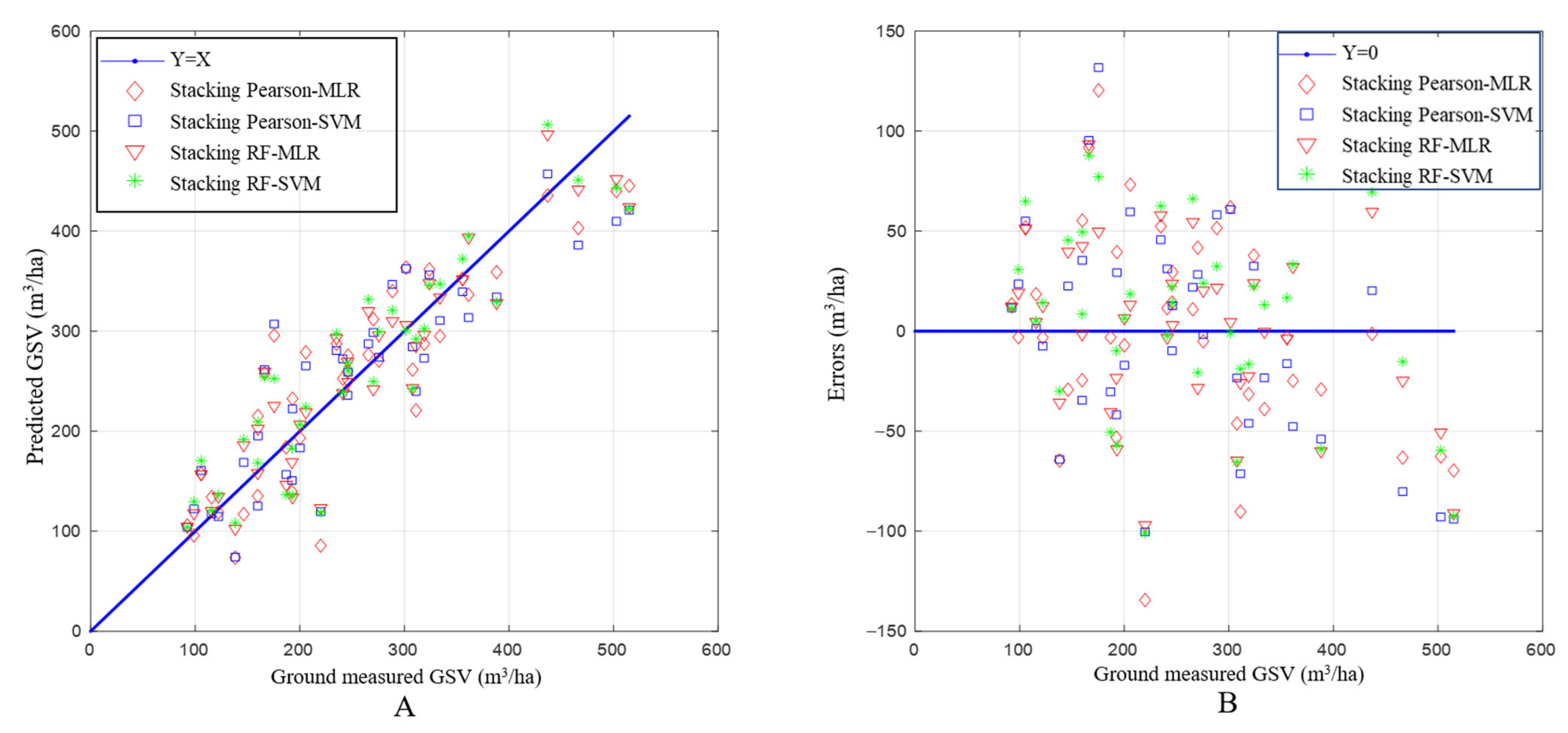
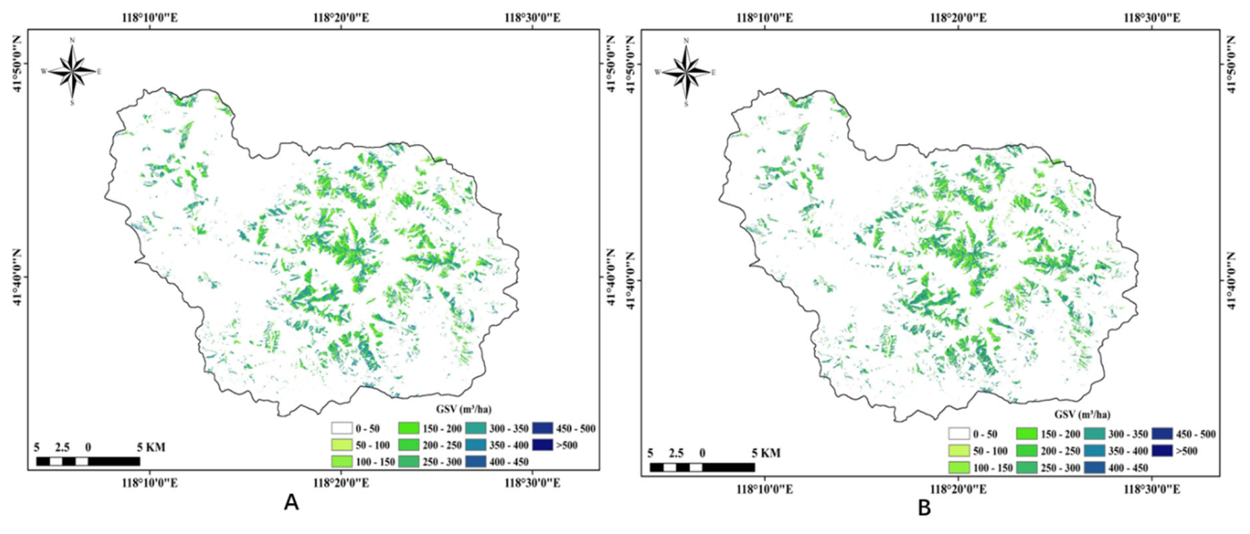
4.4. Estimated GSV from Stacking Resemble Models

In order to overcome the shortages of the single base model, the stacking resemble learning method with various meta-learnings is regarded as an effective way to obtain more accurate forest GSV. In this study, two meta-learnings (MLR and SVM with a linear kernel) were applied to obtain the results based on predicted forest GSV using several base models with various feature sorting methods and FS methods. To further analyze strategies of the stacking ensemble approach, the various sets were constructed based on feature sorting methods, feature selection methods, and meta-learning methods. For each feature sorting method, there were ten sets with various predicted numbers. The results of accuracy indices with various stacking ensemble strategies were listed in

Table 5. The results of accuracy indices derived from various stacking ensemble strategies.

Feature Sorting	Meta-Learning	Stacking Ensemble Learning	RMSE (m3/ha)	rRMSE (%)	Predicted Number
Pearson correlation	MLR	Pearson-MLR	52.08	20.46	4
		Pearson-KNN	63.69	25.03	4
		Pearson-SVM	71.61	28.14	4
		Pearson-RF	63.06	24.78	4
		Pearson-All	51.55	20.26	16
	SVM	Pearson-MLR	47.67	18.74	4
		Pearson-KNN	63.87	25.10	4
		Pearson-SVM	71.85	28.24	4
		Pearson-RF	59.26	23.29	4
		Pearson-All	46.13	18.13	16
Importance of RF	MLR	RF-MLR	52.16	20.50	4
		RF-KNN	81.48	32.02	4
		RF-SVM	65.34	25.68	4
		RF-RF	54.37	21.37	4
		RF-All	42.52	16.71	16
	SVM	RF-MLR	49.90	19.61	4
		RF-KNN	82.74	32.51	4
		RF-SVM	66.02	25.95	4
		RF-RF	53.42	20.99	4
		RF-All	45.82	18.01	16

.

It is illustrated that the accuracy of inverted forest GSV was significantly improved after using stacking ensemble learning with various strategies. Using Pearson correlation for feature sorting, the rRMSE values ranged from 20.26% to 28.24% within four predicted GSV in each feature selection method, and for two different meta-learnings, rRMSE values were 20.26% for MLR and 18.13% for SVM, respectively. It is also found that the accuracy of results is only weakly influenced by the meta-models for construction stacking ensemble learning, and the difference in rRMSE values is within 2%. Moreover, the results derived from the feature sorting with the importance of RF are consistent with those from the feature sorting with Pearson correlation. Additionally, using sixteen predicted GSVs from various feature selection methods in each feature sorting method, the accuracy of the results is higher than using four predicted GSVs by one feature selection method, and the rRMSE values ranged from 16.71% to 20.51%. It is inferred that the accuracy of stacking ensemble learning is highly related to the number of predicted GSVs and the capability of base models.

In this study, the scatterplots between predicted and ground-measured GSV were illustrated to further analyze the results of stacking ensemble learning with different strategies (Figure 7A). After using stacking ensemble learning with two meta-models, the gaps between estimated GSV with different feature sorting methods significantly decreased. Furthermore, both the number of samples with overestimation and underestimation has been largely alleviated. In addition, the systematic distribution of errors between predicted and ground-measured GSV was obviously broken (Figure 7B). After obtaining appropriate models using various strategies, the maps of forest GSV were derived from the stacking ensemble learning with MLR using two feature sorting methods (Figure 8). The results showed that the distributions of mapped forest GSV were basically the same and used different strategies.

5. Discussion

5.1. The Sensitivity of Features Extracted from Dual-Polarization GF-3 Images

Overall, the backscattering coefficients of dual-polarization GF-3 images obtained in this study are in agreement with previous results reported by other studies conducted with other dual or quad SAR images in different sites [31,32,39]. In planted Chinese pine forests, backscattering coefficients ranged from −20 dB to −12 dB for HH polarization, and from −27 dB to −18 dB for HV polarization, respectively. Furthermore, the exponential distribution of backscattering coefficients with various levels of forest GSV conformed to the water cloud model (Figure 4C,D). Simultaneously, the saturation phenomenon of forest GSV still occurred at the level of nearly 300 m³/ha. Because of the acquired date and forest type, the results extracted from dual-polarization GF-3 images seem to be slightly better than the other results extracted from other C band SAR images, such as Sentinel-1.

Moreover, it is necessary to obtain enough alternative feature sets with high sensitivity related to forest GSV [22,23]. Limiting to the polarization modes, backscattering coefficients with different polarizations and features derived from the C2 matrix (non-coherent covariance matrix) are commonly extracted from dual-polarization SAR images [25,31,32]. Among these features, it is concluded that backscattering coefficients of HV polarization mode related to the forest canopy showed high sensitivity to the forest GSV. Although several features can be extracted from C2 matric by dual decomposition approaches, the sensitivity between the forest GSV and extracted features is so low that it cannot be involved in the estimation of forest GSV [31,42,43]. In addition, textural features obtained by GLCM are widely extracted from intensity images of different polarizations for vegetation classification. The previous results confirmed that using SAR textural features improved the discrimination capability of different classes.

In addition to backscattering coefficients and widely used textural features, several derived features related to backscattering coefficients by mathematical operations were constructed to enlarge the number of alternative feature sets. The results showed that some derived features (C9, C10, and C14) showed high sensitivity to the forest GSV (Figure 5). The optimal feature sets also illustrated that these derived features had the exciting potential to improve the accuracy of mapping forest GSV (Table 3). Furthermore, based on the results of base models using optimal feature sets (Table 4), the accuracy of mapping forest GSV using dual-polarization GF-3 images is consistent with the results of other C band SAR images.

For comparing the results with different optimal feature sets, the scatterplots of errors between predicted and ground-measured with different feature sorting methods, different feature selection methods, and base models, were illustrated in Figure 9. The distribution of errors showed that over-estimated results occurred for young forests and under-estimated results occurred for mature or over-mature forests. Normally, this is a common problem that widely occurrs in mapping forest GSV, whether using optical or SAR data. Overall, dual-polarization GF-3 images have great capability to map forest GSV, but these common problems, such as the saturation phenomenon, still occurred at the same time.

5.2. The Potential of the Stacking Ensemble Learning Approach

The accuracy of mapping forest GSV depended on the employed models. Up to now, many models, including MLR, CART, RF, K-NN, SVM, and ANN, are widely used to construct the relationships between selected features and forest parameters [11,25,31,37]. The previous results frequently showed that the performances of these models varied with tree species, images, and selected feature sets. Even for the same optimal feature set, the gaps between various models are highly significant [8,41,44]. The inconsistent results between various models seriously hinder the further application in mapping forest GSV using remote sensing images. Normally, the gaps are induced by the uncertainty of images, forest types, and models, and it is still difficult to reduce the gaps caused by images and forest types. In this study, four base models (MLR, KNN, SVM, and RF) were used to estimate the forest GSV, and the results illustrated that the accuracy of mapped forest GSV varied with feature sorting methods, feature selection methods, and employed models. Even the difference in the values of rRMSE is larger than 10 percentage points. When using the same images covered in the same forest, the gaps between various models are mainly caused by the capability of models and feature selection methods. Thereby, to overcome the gaps induced by optimal feature sets and employed models, ensemble learning algorithms are an effective way to reduce the difference [38,45].

In this study, stacking ensemble learning with different strategies was constructed using various feature selection methods and base models, and the values of rRMSE obtained from all base models and stacking ensemble learning with various strategies are illustrated in Figure 10. When using the same optimal feature set, the uncertainty of mapped forest GSV was caused by models, and the highest and the lowest rRMSE were obtained by RF and KNN, respectively. Essentially, the RF model is one of the ensemble learning models with the same base model using multiple decision trees, and the advantages of ensemble learning have been illustrated for the same optimal feature set (Figure 10).

For different predicted results obtained by various feature sorting and feature selection methods, stacking ensemble learning with various strategies was constructed and the accuracy of mapped forest GSV was obviously improved. Moreover, the gaps in estimated GSV using stacking strategies between feature selection methods decreased. Meanwhile, it is confirmed that the accuracy of the stacking ensemble learning approach was related to the number of predicted results. To further analyze the capability of stacking ensemble learning, the maps of forest GSV were inverted with various stacking strategies, and then the difference of mapped forest GSV was obtained to observe the gaps between various ensemble strategies (

Table 6. Statistical table of the absolute value of errors between A and B obtained from various stacking strategies with different meta-learnings.

Stacking Strategies	Absolute Value of Errors (A–B)
	A	B	<50 m3/ha	(51–100) m3/ha	(101–150) m3/ha	>150 m3/ha
Feature selection	Pearson-MLR(MLR)	RF-MLR(MLR)	1.72%	38.77%	26.66%	34.56%
Feature selection	Pearson-KNN(MLR)	RF-KNN(MLR)	0.00%	46.99%	34.64%	18.37%
Feature selection	Pearson-RF(MLR)	RF-RF(MLR)	0.00%	46.35%	30.45%	23.20%
Feature selection	Pearson-MLR(SVM)	RF-MLR(SVM)	0.00%	38.21%	26.27%	35.53%
Feature selection	Pearson-KNN(SVM)	RF-KNN(SVM)	0.00%	51.79%	32.84%	15.36%
Feature selection	Pearson-RF(SVM)	RF-RF(SVM)	0.00%	46.82%	29.38%	23.80%
Feature selection	Pearson-MLR(SVM)	RF-RF(MLR)	0.00%	43.90%	28.04%	28.06%
Feature selection	Pearson-MLR(SVM)	RF-RF(SVM)	0.00%	38.13%	27.21%	34.66%
Feature selection	Pearson-MLR(SVM)	RF-SVM(MLR)	0.00%	42.19%	25.21%	32.60%
Feature selection	Pearson-MLR(SVM)	RF-SVM(SVM)	0.00%	34.32%	29.38%	36.30%
Feature soring	Pearson-All(MLR)	RF-All(MLR)	0.04%	55.54%	26.89%	17.57%
Feature soring	Pearson-All(SVM)	RF-All(SVM)	0.00%	66.60%	24.78%	8.62%

). The errors between two inverted GSVs obtained with different approaches showed the advantages of stacking ensemble learning, and the reliability of mapped GSVs were highly related to stacking strategies. It was also inferred that the accuracy and reliability of results depended on the number of predicted results from the base models. The percentage of absolute errors (less than 150 m³/ha) obtained by stacking strategies with feature sorting (ranging from 82.43 to 91.38%) is obviously higher than that obtained by stacking strategies with feature selection (ranging from 63.70 to 84.64%). It was also proven that the mapped GSV largely depended on the feature sorting and feature selection methods, and the stacking ensemble learning approach had the potential to reduce the dependence on feature selection methods and models.

6. Conclusions

In this study, dual-polarization GF-3 SAR images (HH, HV) were employed to evaluate the potential of mapping forest GSV in evergreen coniferous forests. Optimal feature sets selected from several proposed derived features and texture features were obtained by various feature sorting and feature selection methods. The maps of forest GSV were derived by stacking ensemble learning approaches with different strategies. The results demonstrated that backscattering coefficients and some related derived features showed high sensitivity to the forest GSV, and the saturation phenomenon also obviously occurred once the forest GSV was larger than 300 m³/ha. Furthermore, the gaps between inverted forest GSV with different models are striking. The accuracy of mapped forest GSV is significantly increased using stacking ensemble learning approaches with different strategies, and the values of rRMSE obtained from stacking ensemble learning within feature sorting methods ranged from 16.71% to 20.51%. This confirms that dual-polarization GF-3 images have great potential to map forest GSV in planted forests, and the gaps between various feature selection methods and models can also be reduced by stacking ensemble learning approaches. However, the uncertainty of tree species and orbit errors related to GF-3 images were not considered in this study. In the future, more tree species, more SAR images from different seasons, and the capability of combination with multi-band SAR images will be further studied.

References

1. Cartus, O.; Santoro, M.; Kellndorfer, J. Mapping forest aboveground biomass in the Northeastern United States with ALOS PALSAR dual-polarization L-band. Remote Sens. Environ. 2012, 124, 466–478. [Google Scholar] [CrossRef]
2. Chowdhury, T.A.; Thiel, C.; Schmullius, C. Growing stock volume estimation from L-band ALOS PALSAR polarimetric coherence in Siberian forest. Remote Sens. Environ. 2014, 155, 129–144. [Google Scholar] [CrossRef]
3. Kobayashi, A.S.; Sanga-Ngoie, K.; Widyorini, R.; Kawai, S.; Omura, Y.; Supriadi, B. Backscattering characteristics of L-band polarimetric and optical satellite imagery over planted acacia forests in Sumatra, Indonesia. J. Appl. Remote Sens. 2012, 6, 063525. [Google Scholar]
4. Suzuki, R.; Kim, Y.; Ishii, R. Sensitivity of the backscatter intensity of ALOS/PALSAR to the above-ground biomass and other biophysical parameters of boreal forest in Alaska. Polar Sci. 2013, 7, 100–112. [Google Scholar] [CrossRef]
5. Thiel, C.; Schmullius, C. Investigating ALOS PALSAR interferometric coherence in central Siberia at unfrozen and frozen conditions: Implications for forest growing stock volume estimation. Can. J. Remote Sens. 2013, 39, 232–250. [Google Scholar] [CrossRef]
6. Li, X.; Lin, H.; Long, J.; Xu, X. Mapping the Growing Stem Volume of the Coniferous Plantations in North China Using Multispectral Data from Integrated GF-2 and Sentinel-2 Images and an Optimized Feature Variable Selection Method. Remote Sens. 2021, 13, 2740. Available online: https://0-www-mdpi-com.brum.beds.ac.uk/2072-4292/13/14/2740 (accessed on 18 March 2020). [CrossRef]
7. Tang, C.; Ye, Z.; Long, J.; Liu, Z.; Zhang, T.; Xu, X.; Lin, H. Mapping forest and site quality of planted Chinese fir forest using sentinel images. Front. Plant Sci. 2022, 13, 949598. Available online: https://www.frontiersin.org/articles/10.3389/fpls.2022.949598 (accessed on 18 March 2020). [CrossRef] [PubMed]
8. Xu, X.; Lin, H.; Liu, Z.; Ye, Z.; Li, X.; Long, J. A Combined Strategy of Improved Variable Selection and Ensemble Algorithm to Map the Growing Stem Volume of Planted Coniferous Forest. Remote Sens. 2021, 13, 4631. [Google Scholar] [CrossRef]
9. Ningthoujam, R.; Balzter, H.; Tansey, K.; Feldpausch, T.; Mitchard, E.; Wani, A.; Joshi, P. Relationships of S-Band Radar Backscatter and Forest Aboveground Biomass in Different Forest Types. Remote Sens. 2017, 9, 1116. [Google Scholar] [CrossRef]
10. Sasan, V.; Javad, S.; Kamran, A.; Hadi, F.; Hamed, N.; Tien, P.; Dieu, T.B. Improving Accuracy Estimation of Forest Aboveground Biomass Based on Incorporation of ALOS-2 PALSAR-2 and Sentinel-2A Imagery and Machine Learning: A Case Study of the Hyrcanian Forest Area (Iran). Remote Sens. 2018, 10, 172. [Google Scholar]
11. Zhu, Y.; Liu, K.; Myint, S.W.; Du, Z.; Wu, Z. Integration of GF2 Optical, GF3 SAR, and UAV Data for Estimating Aboveground Biomass of China’s Largest Artificially Planted Mangroves. Remote Sens. 2020, 12, 2039. [Google Scholar] [CrossRef]
12. Long, J.; Lin, H.; Wang, G.; Sun, H.; Yan, E. Mapping Growing Stem Volume of Chinese Fir Plantation Using a Saturation-based Multivariate Method and Quad-polarimetric SAR Images. Remote Sens. 2019, 11, 1872. [Google Scholar] [CrossRef]
13. Li, X.; Ye, Z.; Long, J.; Zheng, H.; Lin, H. Inversion of Coniferous Forest Stock Volume Based on Backscatter and InSAR Coherence Factors of Sentinel-1 Hyper-Temporal Images and Spectral Variables of Landsat 8 OLI. Remote Sens. 2022, 14, 2754. Available online: https://mdpi-res.com/d_attachment/remotesensing/remotesensing-14-02754/article_deploy/remotesensing-14-02754-v3.pdf?version=1654843806 (accessed on 18 March 2020). [CrossRef]
14. Wang, Z.M.; Zhang, W.Q.; Yue, C.R.; Liu, Q. Estimation of Forest Growing Stock Based on TerraSAR-X and ALOS PALSAR Data: A Case Study in Mengla County of Yunnan Province. J. Zhejiang For. Sci. Technol. 2018, 38, 38–43. [Google Scholar]
15. Kobayashi, S.; Omura, Y.; Sanga-Ngoie, K.; Yamaguchi, Y.; Widyorini, R.; Fujita, M.S.; Supriadi, B.; Kawai, S. Yearly Variation of Acacia Plantation Forests Obtained by Polarimetric Analysis of ALOS PALSAR Data. IEEE J. Sel. Top. Appl. Earth Obs. Remote Sens. 2016, 8, 5294–5304. [Google Scholar] [CrossRef]
16. Santoro, M.; Wegmuller, U.; Fransson, J.E.S.; Schmullius, C. Regional mapping of forest growing stock volume with multitemporal ALOS PALSAR backscatter. In Proceedings of the 2014 IEEE Geoscience & Remote Sensing Symposium, Quebec City, QC, Canada, 13–18 July 2014. [Google Scholar]
17. Stelmaszczuk-Górska, M.; Rodriguez-Veiga, P.; Ackermann, N.; Thiel, C.; Balzter, H.; Schmullius, C. Non-Parametric Retrieval of Aboveground Biomass in Siberian Boreal Forests with ALOS PALSAR Interferometric Coherence and Backscatter Intensity. J. Imaging 2015, 2, 1. [Google Scholar] [CrossRef]
18. Thiel, C.; Schmullius, C. Impact of Tree Species on Magnitude of PALSAR Interferometric Coherence over Siberian Forest at Frozen and Unfrozen Conditions. Remote Sens. 2014, 6, 1124–1136. [Google Scholar] [CrossRef]
19. Thiel, C.; Schmullius, C. The potential of ALOS PALSAR backscatter and InSAR coherence for forest growing stock volume estimation in Central Siberia. Remote Sens. Environ. 2016, 173, 258–273. [Google Scholar] [CrossRef]
20. Antropov, O.; Rauste, Y.; Häme, T.; Praks, J. Polarimetric ALOS PALSAR Time Series in Mapping Biomass of Boreal Forests. Remote Sens. 2017, 9, 999. [Google Scholar] [CrossRef]
21. Joshi, N.; Mitchard ET, A.; Brolly, M.; Schumacher, J.; Fernándezlanda, A.; Johannsen, V.K.; Marchamalo, M.; Fensholt, R. Understanding ‘saturation’ of radar signals over forests. Sci. Rep. 2017, 7, 3505. [Google Scholar] [CrossRef] [PubMed]
22. Zhang, H.; Zhu, J.; Wang, C.; Lin, H.; Long, J.; Zhao, L.; Fu, H.; Liu, Z. Forest Growing Stock Volume Estimation in Subtropical Mountain Areas Using PALSAR-2 L-Band PolSAR Data. Forests 2019, 10, 276. Available online: https://0-www-mdpi-com.brum.beds.ac.uk/1999-4907/10/3/276 (accessed on 18 March 2020). [CrossRef]
23. Ataee, M.S.; Maghsoudi, Y.; Latifi, H.; Fadaie, F. Improving Estimation Accuracy of Growing Stock by Multi-Frequency SAR and Multi-Spectral Data over Iran’s Heterogeneously-Structured Broadleaf Hyrcanian Forests. Forests 2019, 10, 641. [Google Scholar] [CrossRef]
24. Wan, Y.; Guo, S.; Li, L.; Qu, X.; Dai, Y. Data Quality Evaluation of Sentinel-1 and GF-3 SAR for Wind Field Inversion. Remote Sens. 2021, 13, 3723. [Google Scholar]
25. Wang, G.; Wang, N.; Guo, W. Modelling Forest Aboveground Biomass Based on GF-3 Dual-Polarized and WorldView-3 Data: A Case Study in Datong National Wetland Park, China. Mathematical Problems in Engineering: Theory, Methods and Applications. Math. Probl. Eng. 2021, 2021, 1–13. [Google Scholar]
26. Yin, J.; Yang, J.; Zhang, Q. Assessment of GF-3 Polarimetric SAR Data for Physical Scattering Mechanism Analysis and Terrain Classification. Sensors 2017, 17, 2785. [Google Scholar] [CrossRef]
27. Karila, K.; Vastaranta, M.; Karjalainen, M.; Kaasalainen, S. Tandem-X interferometry in the prediction of forest inventory attributes in managed boreal forests. Remote Sens. Environ. 2015, 159, 259–268. [Google Scholar] [CrossRef]
28. Mermoz, S.; Réjou-Méchain, M.; Villard, L.; Toan, T.L.; Rossi, V.; Gourlet-Fleury, S. Decrease of L-band SAR backscatter with biomass of dense forests. Remote Sens. Environ. 2015, 159, 307–317. [Google Scholar] [CrossRef]
29. Santoro, M.; Beaudoin, A.; Beer, C.; Cartus, O.; Fransson JE, S.; Hall, R.J.; Pathe, C.; Schmullius, C.; Schepaschenko, D.; Shvidenko, A. Forest growing stock volume of the northern hemisphere: Spatially explicit estimates for 2010 derived from Envisat ASAR. Remote Sens. Environ. 2015, 168, 316–334. [Google Scholar] [CrossRef]
30. Yu, Y.; Saatchi, S. Sensitivity of L-Band SAR Backscatter to Aboveground Biomass of Global Forests. Remote Sens. 2016, 8, 522. [Google Scholar] [CrossRef]
31. Santoro, M.; Cartus, O.; Fransson JE, S.; Wegmüller, U. Complementarity of X-, C-, and L-band SAR Backscatter Observations to Retrieve Forest Stem Volume in Boreal Forest. Remote Sens. 2019, 11, 1563. [Google Scholar] [CrossRef]
32. Hongquan, W.; Ramata, M.; Kalifa, G.T. Potential of a two-component polarimetric decomposition at C-band for soil moisture retrieval over agricultural fields. Remote Sens. Environ. 2018, 217, 38–51. [Google Scholar]
33. Kiyohara, B.H.; Sano, E.E. Mapping Secondary Vegetation of a Region of Deforestation Hotspot in the Brazilian Amazon: Performance Analysis of C- and L-Band SAR Data Acquired in the Rainy Season. Forests 2022, 13, 1457. Available online: https://0-www-mdpi-com.brum.beds.ac.uk/1999-4907/13/9/1457 (accessed on 18 March 2020). [CrossRef]
34. Qin, Z.; Ni, L.; Tong, Z.; Qian, W. Deep Learning Based Feature Selection for Remote Sensing Scene Classification. IEEE Geosci. Remote Sens. Lett. 2015, 12, 2321–2325. [Google Scholar]
35. Di Cosmo, L.; Gasparini, P.; Tabacchi, G. A national-scale, stand-level model to predict total above-ground tree biomass from growing stock volume. For. Ecol. Manag. 2016, 361, 269–276. [Google Scholar] [CrossRef]
36. Yu, T.; Pang, Y.; Liang, X.J.; Jia, W.; Bai, Y.; Fan, Y.L.; Chen, D.S.; Liu, X.Z.; Deng, G.; Li, C.G.; et al. China’s larch stock volume estimation using Sentinel-2 and LiDAR data. Geo-Spatial Inf. Sci. 2022, 1–14. [Google Scholar] [CrossRef]
37. Song, S. Land Cover Classification with Multispectral LiDAR Based on Multi-Scale Spatial and Spectral Feature Selection. Remote Sens. 2021, 13, 4118. [Google Scholar]
38. Singh, C.; Karan, S.K.; Sardar, P.; Samadder, S.R. Remote sensing-based biomass estimation of dry deciduous tropical forest using machine learning and ensemble analysis. J. Environ. Manag. 2022, 308, 114639. [Google Scholar] [CrossRef]
39. Zhang, X.; Xu, J.; Chen, Y.; Xu, K.; Wang, D. Coastal Wetland Classification with GF-3 Polarimetric SAR Imagery by Using Object-Oriented Random Forest Algorithm. Sensors 2021, 21, 3395. [Google Scholar] [CrossRef] [PubMed]
40. Suzuki, K.; Laohakangvalvit, T.; Matsubara, R.; Sugaya, M. Constructing an Emotion Estimation Model Based on EEG/HRV Indexes Using Feature Extraction and Feature Selection Algorithms. Sensors 2021, 21, 2910. [Google Scholar] [CrossRef] [PubMed]
41. Li, X.; Long, J.; Zhang, M.; Liu, Z.; Lin, H. Coniferous Plantations Growing Stock Volume Estimation Using Advanced Remote Sensing Algorithms and Various Fused Data. Remote Sens. 2021, 13, 3468. [Google Scholar] [CrossRef]
42. Guo, X.; Li, K.; Yun, S.; Wang, Z.; Li, H.; Zhi, Y.; Long, L.; Wang, S. Inversion of Rice Biophysical Parameters Using Simulated Compact Polarimetric SAR C-Band Data. Sensors 2018, 18, 2271. [Google Scholar] [CrossRef] [PubMed]
43. Rosa RA, S.; Fernandes, D.; Barreto TL, M.; Wimmer, C.; Nogueira, J.B. Change detection under the forest in multitemporal full-polarimetric P-band SAR images using Pauli decomposition. In Proceedings of the 2016 IEEE International Geoscience and Remote Sensing Symposium (IGARSS), Beijing, China, 10–15 July 2016. [Google Scholar]
44. Jiang, F.; Kutia, M.; Ma, K.; Chen, S.; Long, J.; Sun, H. Estimating the aboveground biomass of coniferous forest in Northeast China using spectral variables, land surface temperature and soil moisture. Sci. Total Environ. 2021, 785, 147335. Available online: https://0-www-sciencedirect-com.brum.beds.ac.uk/science/article/pii/S0048969721024062 (accessed on 18 March 2020). [CrossRef] [PubMed]
45. Li, X.; Zhang, M.; Long, J.; Lin, H. A Novel Method for Estimating Spatial Distribution of Forest Above-Ground Biomass Based on Multispectral Fusion Data and Ensemble Learning Algorithm. Remote. Sens. 2021, 13, 3910. [Google Scholar] [CrossRef]
Figure 1. Study area and the distribution map of ground-measured Chinese pine samples.
Remotesensing 15 02253 g001
Figure 2. Intensity images of GF-3 dual-polarization SAR data and slope map in the study area.
Remotesensing 15 02253 g002
Figure 3. Framework for mapping planted forest GSV based on the stacking ensemble learning using dual-polarization GF-3 SAR images.
Remotesensing 15 02253 g003
Figure 4. The scatterplots between partial features and forest GSV; the meanings and formulas of mentioned features were shown in Table 1. (AI) are SHH, SHV, σHV, σHH, C1, C5, C8, C9 and C11 respectively.
Remotesensing 15 02253 g004
Figure 5. Pearson correlation coefficient (γ > 0.2) between alternative variables and forest GSV.
Remotesensing 15 02253 g005
Figure 6. Scatterplots between ground-measured and predicted GSV using four feature selection methods by various feature sorting methods and base models. (AD) Is the results derived from the feature sorting method with Pearson correlation and (EH) is the results derived from the feature sorting method with the importance of RF.
Remotesensing 15 02253 g006
Figure 7. (A) Scatterplots between ground-measured and predicted GSV obtained from various stacking ensemble learning strategies and (B) scatterplots of errors obtained from various stacking ensemble learning strategies.
Remotesensing 15 02253 g007
Figure 8. The maps of forest GSV using stacking ensemble learning in planted Chinese pines. (A) Is from the Pearson stacking ensemble learning with MLR and (B) is from the importance stacking ensemble learning with MLR.
Remotesensing 15 02253 g008
Figure 9. The errors between predicted and ground-measured GSV using four base models. (AD) Is the results using Pearson correlation for sorting features and (EH) is the results using the importance of RF for sorting features.
Remotesensing 15 02253 g009
Figure 10. The values of rRMSE from all base models and stacking ensemble learning with various strategies. The red and blue lines indicate the feature sorting method with Pearson correlation and the importance of RF, respectively.
Remotesensing 15 02253 g010