

Multi-Year Time Series Transfer Learning: Application of Early Crop Classification

1
Faculty of Civil and Geodetic Engineering, University of Ljubljana, 1000 Ljubljana, Slovenia
2
Sinergise Solutions, Ltd., 1000 Ljubljana, Slovenia
3
Faculty of Computer and Information Science, University of Ljubljana, 1000 Ljubljana, Slovenia
*
Author to whom correspondence should be addressed.
Remote Sens. 2024, 16(2), 270; https://0-doi-org.brum.beds.ac.uk/10.3390/rs16020270
Submission received: 17 November 2023
/
Revised: 5 January 2024
/
Accepted: 8 January 2024
/
Published: 10 January 2024
(This article belongs to the Special Issue Deep Learning Techniques Applied in Remote Sensing)
Abstract
:Crop classification is an important task in remote sensing with many applications, such as estimating yields, detecting crop diseases and pests, and ensuring food security. In this study, we combined knowledge from remote sensing, machine learning, and agriculture to investigate the application of transfer learning with a transformer model for variable length satellite image time series (SITS). The objective was to produce a map of agricultural land, reduce required interventions, and limit in-field visits. Specifically, we aimed to provide reliable agricultural land class predictions in a timely manner and quantify the necessary amount of reference parcels to achieve these outcomes. Our dataset consisted of Sentinel-2 satellite imagery and reference crop labels for Slovenia spanning over years 2019, 2020, and 2021. We evaluated adaptability through fine-tuning in a real-world scenario of early crop classification with limited up-to-date reference data. The base model trained on a different year achieved an average F1 score of 82.5% for the target year without having a reference from the target year. To increase accuracy with a new model trained from scratch, an average of 48,000 samples are required in the target year. Using transfer learning, the pre-trained models can be efficiently adapted to an unknown year, requiring less than 0.3% (1500) samples from the dataset. Building on this, we show that transfer learning can outperform the baseline in the context of early classification with only 9% of the data after 210 days in the year.
1. Introduction
Land cover classification is an important task in remote sensing with numerous applications in agriculture, environmental monitoring, and land management [1,2]. One of its most important applications is crop classification [3,4], which is essential for many reasons, e.g., expected yield determination, detecting crop diseases and pest impact, and ensuring food security [5]. Recent developments in the field of crop classification using Satellite Image Time Series (SITS) in combination with machine learning [6,7,8] have shown that it is possible to differentiate between different crops before the end of their growth cycle. This is important, as we prefer to have the crop type information available as soon as possible, i.e., in real time. This approach, referred to as early classification or in-season classification, focuses on crop differentiation during their growth cycle. In a real-world scenario, we would like to predict crop types in the same (current) year as quickly as possible. This is a significant challenge due to limited data availability, as crop type information is collected throughout the year and is often not fully available until after the season. This is particularly true for the Common Agricultural Policy (CAP) in the European Union [9]. Most of the studies conducted so far are based on datasets that include only a single year’s data. In addition, there are only a few large-scale crop declaration initiatives worldwide, which underlines the importance of knowing what can be achieved with a limited amount of recent reference data.
This study addresses early crop classification over several years for a large area, i.e., the whole of Slovenia. Slovenia was selected because the reference data for agricultural land use has been made publicly accessible and available for multiple years. In this paper, we examine the role of pre-training and fine-tuning of a transformer architecture [10,11,12,13], which has become the state of the art for deep learning in several fields. We use SITS from individual years to either pre-train the model or to adapt (fine-tune) the model to the target year using a small amount of the partially available SITS.
1.1. Crop Classification
When addressing crop classification, most studies use training and testing data from a dataset limited to a single year [4,14,15,16,17]. The reason for this approach is the limited scope of available sample annotations for crop classification. This means the models are often trained on a single year and thus lack generalization capabilities. Meteorological conditions in the target year can significantly affect vegetation development and impact the SITS temporal signature, resulting in a different temporal signature for the same crop. Some authors have attempted to improve the model’s generalizability by using multiple years to train a single model [18]. More recently, some papers [16,19,20] have explored knowledge transfer between years to address this issue. Weikmann et al. [20] studied knowledge transfer from source to target year and showed that the performance decreases, but when some samples from the target year are added, the model’s performance improves significantly.
Most previous work on early crop classification has focused on classical machine learning methods [6,19,21] with complete SITS for a single year. Some authors [6,7,8] show that the accuracy of early classification also depends on crop type and geographic location. However, the ability to generalize over multiple years has not been thoroughly studied [20]. Marszalek et al. [22] used Random Forest (RF) and Support Vector Machines (SVM), which have shown promise but are not scalable and require re-training for each additional observation with multi-year data.
Deep learning provides a solution to address this problem. As described by Yasir et al. [23], deep learning is already used extensively in remote sensing, including in crop classification. One of the most efficient deep architectures for processing SITS are transformers [11], which can exploit temporal dependencies between different time points. Due to the hierarchical nature of deep models and the iterative way in which they are trained, various knowledge transfer techniques, such as fine-tuning (e.g., [13,24]), can be easily applied to limited datasets. All deep models, including transformer-based architectures, can be optimized and adapted faster to a similar task with good results by using pre-trained weights as a basis. Although a few studies have addressed early crop classification, they were mainly based on Recurrent Neural Networks (RNN) [25], Long Short-Term Memory(LSTM) [26], and similar architectures. The use of transformers was limited to annual time series, making our study the first to use transformers for early crop classification.
1.2. Objectives and Study Layout
The objective of this study was to produce a map of agricultural land, reduce required interventions, and limit in-field visits. The goal is to attain results before the end of the growing period. It is essential to strike a balance, avoiding premature assessments in the current year that may compromise the quality of produced results. Specifically, we aim to provide reliable agricultural land class predictions in a timely manner and quantify the necessary amount of reference parcels to achieve these outcomes.
This paper presents a comprehensive study of temporal generalization in early crop classification using transformer architecture. The study revolves around a real-world scenario where (additional) satellite data continuously becomes available, typically every week, allowing for continuous improvement of the model. Our analysis focuses on comparing models that have been trained from scratch with those that have been pre-trained and fine-tuned using data from the target year. We investigate this using a dataset spanning multiple years for the entire country (Slovenia) and examine the number of samples required, earliness, and contribution of historical data to achieve better crop classification performance. To our knowledge, this is the first study to investigate early crop classification in temporal knowledge transfer scenarios for deep learning models and the first study to investigate transformer architectures with respect to early crop classification.
2. Materials
2.1. Study Area
This study was conducted for the entire country of Slovenia [27], located in Central Europe with a diverse landscape characterized by a complex mosaic of different landscapes due to relief, climate, landscape, and agricultural practices, as seen in Figure 1. In the north, the alpine hills are characterized by meadows and pastures. In the western part, vineyards and olive groves predominate. There is a pronounced agricultural focus in the northeast, where hops are the main crop. The country’s total area is around 20,000 km2, of which 36% is agricultural land. Due to terrain characteristics and land ownership, parcels in Slovenia are often small (on average less than five hectares in size), narrow (less than one Sentinel-2 pixel), long, and irregularly shaped, resulting in high fragmentation. This poses a challenge for crop classification using Sentinel data.
2.2. Reference Data
Reference data were extracted from farmers’ declarations that are provided annually and published by the Ministry of Agriculture, Forestry and Food of Slovenia [28]. The data can be downloaded directly from the ministry website. Our study used the data for the years 2019, 2020, and 2021. The data include over 200 land cover types, which we reclassified into 30 taxonomically similar classes in collaboration with experts from the Agency for Agricultural Markets and Rural Development. Even though the aggregated dataset contains grasslands and fallow land classes, we refer to them as crop classes throughout this study. This terminology aligns with that used in related research, emphasising our focus on distinguishing between various crop types.
These aggregated (major) groups can be found throughout the European Union. The distribution of samples for each reclassified crop group can be seen in Figure 2 for the year 2021. All years, on average, contain 592,000 referenced agricultural parcels (Table A1), with similar class distribution. Most reference samples fall into a few prominent groups, namely maize, followed by vegetables, winter cereals, vineyards, and winter barley. Fourteen smaller classes represent categories with less than 1000 samples (orange), while meadows (green) have 92 times more samples than all smaller classes combined. It is worth noting that this distribution is specific to Slovenia and differs from that of other countries.
The study area was divided into training–validation–testing groups, in the same ways as proposed and named by authors of the SITS-BERT model [11] utilized in this study. We divided the study area into H3 hexagons [29], as shown in Figure 3. We chose hexagons because they offer a consistent division of the Earth’s surface on multiple scales, do not overlap, and provide the technology for efficient large-scale computing [30,31]. Subdivisions were made at the zoom (https://h3geo.org/docs/core-library/restable/, accessed on 5 July 2023) Level 7, which determines the size of the hexagons, with each hexagon covering approximately 5.2 km2 as this best reproduces the original data distribution. Some hexagons, mostly in the mountain regions, were left out because there were few or no crops in the area.
The hexagons were randomly assigned to both the training and testing datasets. The same spatial distribution was used for all years, resulting in a similar class distribution between test and training. We used of the hexagons for training and for testing. During training, of the training dataset was used for validation to select the best model for each run.
2.3. Satellite Image Time Series
Sentinel-2 [32] imagery was used because of its high spatial resolution of 10 m (in B2, B3, B4 and B8, the four bands mainly used for agriculture) and revisit time of 5 days. Based on this imagery, one SITS was generated for each reference parcel. Every parcel was assigned to only one hexagon, belonging to only one-training, testing—data split. Parcels smaller than one Sentinel-2 pixel were excluded because it was not possible to create representative SITS for such small areas. Data were downloaded from the Sentinel Hub (https://sentinel-hub.com, accessed on 5 May 2023), aggregated by parcel and masked. In the data preprocessing step, the atmospherically corrected Sentinel-2 L2A imagery for years 2019, 2020, and 2021 was downloaded from Sentinel Hub. We used the 12 bands of the L2A product, and retrieved also the s2cloudless mask, which provides additional information about cloud cover and offers cloud probability for each pixel. All pixels with cloud probability greater than 0.4 were masked out. After applying the cloud mask, a mixture of valid and undetected anomalous observations (usually caused by cloud shadows, snow, and haze) still remained. To mask such outliers, a LightGBM model, trained specifically on hand-labelled data from agricultural parcels in Slovenia, was used (https://area-monitoring.sinergise.com/docs/signal-processing/, accessed on 23 May 2023).
The remaining valid observations were aggregated for each parcel using the mean of the pixels that were entirely within the parcel boundaries. This ensured that signals from different parcels were not mixed. The final SITS had values for 12 bands, i.e., the mean per parcel for every time. The dataset was structured as shown in Figure 4. Each row consisted of the observed values O for each of the bands B in succession for each observation time t for a single parcel. The corresponding day of year (DOY) t was given for every observation time (total L times) and the agricultural land class for the parcel. The length of each row was different, as we included only valid observations, meaning that L was different for every row.
3. Methodology
In this study, we investigate knowledge transfer and fine-tuning for the classification of SITS using a transformer-based neural network architecture. Our goal is to use large amounts of SITS from previous years to train robust and transferable spectral–temporal features. With the trained models, we can improve the accuracy of annual classification, even in cases where reference information is lacking. We use the term source year on which the pre-training was performed and term target year for the year used to fine-tune the model. The terms source and target are standardly used in the field of computer vision to represent the source dataset used to train the model and the target dataset, which is used for optimizing and evaluating the model’s performance. Assuming a weak correlation between individual years in our dataset, each year can be used interchangeably for both roles.
3.1. Transformers
The machine learning model used in the study is based on the transformer deep neural network architecture [10], and we utilize the transformer implementation SITS-BERT proposed in [11]. The SITS-BERT architecture is composed of two parts, an observation embedding layer and a transformer encoder, as shown in Figure 5. The authors that developed the architecture used a self-supervised pre-training scheme to train the model. The scheme uses extensive unlabelled data to learn general spectral–temporal representations of land cover semantics. The pre-trained network is then fine-tuned using smaller task-related referenced data to adapt to different SITS classification tasks. This approach has been shown to improve classification accuracy and reduce the risk of overfitting.
The self-supervised pre-training step is skipped in our study since historical data are available, and the study focuses on knowledge transfer between years. To this end, we adjust the training process to examine the importance of the referenced samples on the obtained results. In addition, transformers can use partially available time series data of different lengths, meaning the SITS do not need to be preprocessed to the same interval, as is the case with RF and SVM. This makes transformers a better choice for early crop classification than RF and SVM.
3.2. Evaluation Metrics
We used the most commonly used evaluation metrics, i.e., the Overall Accuracy (OA) [6,8] and F1 score [7,19,20] that both summarize global model performance. OA represents the proportion of correctly classified samples by dividing the number of all correctly classified samples by the number of all referenced samples in the dataset. The F1 score, on the other hand, combines two metrics, precision and recall, into a single measure. Precision is the fraction of relevant instances among the retrieved instances, it is calculated as the number of correctly classified samples (true positives) divided by the number of both correctly and incorrectly classified samples (true positives and false positives). Recall is the fraction of relevant instances that were retrieved, it is the number of correctly classified samples (true positives) divided by the number of all samples for the specific class (true positives and false negatives).
Both metrics range from 0 to 1, with higher values indicating better performance. We focus on the F1 score because it accounts for false positives and false negatives. In other words, it considers both a model’s ability to correctly classify instances of one class and its ability not to misclassify instances of other classes as that class. The weighted F1 score, which calculates the F1 score for each class and then takes the average weighted by the number of instances in each class, is used in our study. In this way, higher importance is given to the more abundant crops and shows how well the model performs at the country level rather than the individual crop level.
To gain further insight, we used a confusion matrix to show how well the model performs in each class and where it has problems. The matrix consists of all available samples and classes ordered by the correct and predicted class, with the diagonal values representing the correct predictions and outside the diagonal are samples the model predicted wrong. When looking at the confusion matrix, one must also consider the specific characteristics of the dataset and the problem when interpreting the results.
3.3. Testing Layout
We designed a series of experiments to analyse the data and the models. These experiments aimed to evaluate the effects of temporal generalization, transfer learning, and early classification on the model’s performance and to gain insights useful for future research in this area. The experiments were divided into four groups:
- Temporal generalization: to assess the extent to which the model could generalize across different years and the importance of prior knowledge, we tested the model’s performance for each year. The trained weights were used in subsequent experiments.
- Undersampling: the effects of a limited sample size, assessed by randomly selecting a subset of the available data and reducing the sample size to a fraction of the total. This allowed for us to examine the model’s performance under conditions of limited data availability.
- Transfer learning: building on the experiments of undersampling and temporal generalization, we investigated how to optimize the model with limited reference data. We used a pre-trained model and undersampled the available data to simulate the scarcity of reference data and to determine the minimum number of samples required to obtain comparable results as with the entire dataset. By combining these experiments, we gained insight into the model’s ability to handle limited data and adapt to the classification scenario for a different year, ultimately optimizing the model for the real-world use case.
- Early classification: combining all the previously mentioned experiments and evaluating the impact of limited temporal information on the model’s performance by gradually adding more data to the model as it became available over time. Simulating a real world in which new observations become available (over the course of the year). In this way, we gain insights into how the model can be used for early crop classification.
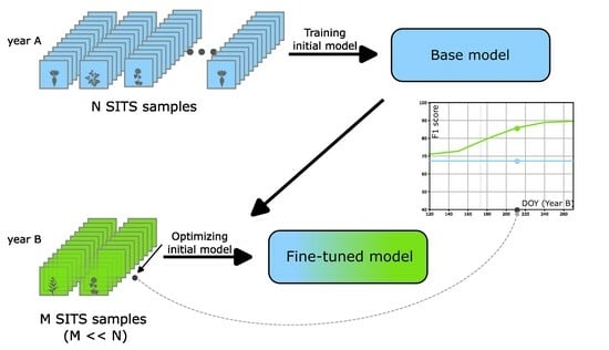
The procedure is illustrated in Figure 6, where the initial model was trained separately for each year and evaluated on all years to establish the baseline that serves as a reference for all other evaluations. We optimized the produced models for a different year to create a fine-tuned model with a reduced sample size. In the final step, we also reduced the available temporal information to evaluate the model’s performance in the context of early classification. The procedure is applied for all combinations, e.g., in Combination 2 in the Figure 6, the year 2020 was used to train the initial model, and the model was evaluated on both 2019 and 2021 to establish the baseline. This model was then fine-tuned with a subset of 2019 and 2021 datasets individually, while the temporal information was also reduced to simulate early classification.
The following hyperparameter settings were used for all models: the maximum sequence length was increased to 127, and the number of classes was set to 30. After extensive experimentation with different parameters, the learning rate was set to since it provided the best results on average. We also reduced the number of epochs to 100 and increased the batch size to 1500 to optimize training efficiency. To prevent overfitting and ensure the model’s stability, we stopped training early if the F1 score on the validation dataset did not improve after 15 epochs. The rest of the model’s parameters were not changed and are consistent with the authors’ original proposal [11].
These specific hyperparameters were maintained for all runs to provide a standardized framework for comparison and to ensure reliability and reproducibility between runs. The training and optimization procedures were performed on three RTX 2080 Ti GPUs, with the total training time spanning more than 205 days.
4. Results
The chapter is divided into four parts, following the same structure as described in Section 3.3. Based on temporal generalization, we establish a baseline, which serves as a reference for all subsequent experiments. We continue with undersampling, where we investigate the impact of limiting the available training samples on the model’s performance. Using transfer learning, we build on these findings, and compare the results obtained by fine-tuning the models trained on a source year with the data from the target year. Combining all these finding for early classification, we determine the earliest time at which these results can be provided.
4.1. Temporal Generalization
To ensure the comparability of the models for different years, the training parameters were kept the same for all experiments. The results of the temporal generalization experiment are summarized in Table 1 using F1 score. All models achieved an F1 score above 91% for the observed year, as seen at the diagonal values in the table. Comparing the average of the rows for all years, the models trained on 2019 and 2021 achieved similar performance, with the performance of the model trained on the year 2020 standing out. The model was able to achieve only slightly lower performance in the training year, but was able to generalize better to the target years. When comparing test performance by averaging the columns, the models for the different years were able to achieve 85.4% of the F1 score. If the year for which the model was trained was excluded, the performance dropped to 82.5%. This score was a baseline of what can be expected from a model’s performance for a target year. We included it in the following visualizations to determine when model performance exceeds this value.
4.2. Undersampling and Transfer Learning
In the experiments, training was performed with a different number of available samples to investigate how these different quantities affect model performance. Figure 7 visually represents the correlation between performance and the increasing number of samples used for training in each iteration. As expected, increasing the sample size consistently led to improved performance on the test dataset. The model in blue was trained from scratch. The model trained with the original distribution (solid line) outperformed the baseline (red line) when we used at least 48,000 samples. All subsequent steps included double the number of samples and only a slight performance improvement.
We also investigated the effects of the training data distribution on model performance. Two lines of the same colour are distinguished by the distribution of the training data. The solid line represents the model trained on the original distribution of the available data (original). In contrast, the dotted line represents the model trained on a distribution with an equal number of samples for all classes (equal), if available. The model’s performance with equal class distribution starts at almost 0% when all classes have the same number of samples. However, the model’s performance is comparable to the original distribution (solid line) after training with 5000 samples. The gap between the two distributions increases again after 12,000 samples and converges after 100k samples.
Figure 7 visualizes a pre-trained model (orange) performance with equal distribution next to the original distribution, measured by the F1 score. The pre-trained models always perform better than the corresponding models trained from scratch (blue). The two solid lines differ by 33% when 1500 samples are used. However, when the sample size increases to 48,000 samples, the difference decreases to less than 5%. Similar to before, the model was trained with an increasing amount of samples from a target year. In the case of pre-training (solid orange), the baseline can be outperformed with only 1500 samples (less than 0.3% of the original dataset). When we increased the size to 12,000 samples, the standard deviation of the solid orange line dropped below 1%, leading to consistent results between runs.
4.3. Early Classification
We know from previous experiments that we can obtain reliable results with pre-trained models and fine-tuning with only 12,000 samples when SITS are available for the whole year. The results change if the SITS are not available for the entire year. By adding the observations as they become available (all observations up to the specified DOY), we can simulate the progression of a year. As shown in Figure 8a, the average performance from 12,000 samples (blue) is only above 50% before the 200 DOY. Still, it increases steadily as the year progresses and more data become available. After the end of August, at the 240 DOY, the model’s performance exceeds the baseline. In other words, by fine-tuning a model with 12,000 samples, we can provide reliable results after the 240 DOY mark. By increasing the number of samples to 24,000 (orange), one can observe an improvement in overall performance. The average performance up to 200 DOY is now always above 60%, and the model exceeds the baseline slightly earlier and shows a few percent improvements at the 240 DOY mark compared to the use of only 12,000 samples. However, the most significant improvement can be observed with 48,000 samples (green). The performance is already above 70% at the beginning of May (120 DOY). At 210 DOY, at the end of July, the model already exceeds the baseline (82.5%) determined in Section 4.1. The model performs well for groups with more samples (meadows, maize, winter cereals) but confuses similar groups, such as roses and ornament plants. The complete confusion matrix can be found in the Appendix see Figure A1.
Looking at the standard deviations of the models shown in Figure 8a and plotting them in Figure 8b, revealing patterns emerge. The models with 12,000 and 24,000 samples have a high standard deviation up to the 240 DOY mark. In contrast, the standard deviation of the 48,000 model decreases significantly already before 180 DOY.
To illustrate the change in predictions produced by the model, we increase the temporal information until each DOY in Figure 9 and show the change in predictions over the course of the year for a selected parcel. We choose a parcel where the class changes several times, and the visualization is limited to the trend of only the relevant classes. The crop type changes several times from maize to hop, meadow, and then back to maize. Finally, at the 210 DOY mark, it is correctly classified as soybean. As time progresses, the score for most classes decreases while the score for the most likely class increases.
5. Discussion
We demonstrated the applicability of deep learning for crop classification using SITS under the typical conditions of Earth observation, such as limited observations and reference data. Previous research [8,11] has already shown the adaptability of deep learning for different geographical regions and continents. We evaluated the model’s ability to adapt and generalize to target years by capturing temporal crop patterns.
5.1. Temporal Generalization
The result in Table 1 is consistent with the findings of [20], where a decrease in performance of 10% to 14% was observed for the target years. In our study, a decline between 5% and 16% was observed for the target years, depending on the specific year. Our results showed a similarity between 2019 and 2021, as the model identified distinct features for these years that were not present in 2020. The model trained on 2020 had the highest degree of robustness, achieving an average performance of 86.3% on target years. This indicated the model’s strong ability to generalize beyond the training year, demonstrating its effectiveness in adapting to different years.
5.2. Undersampling and Transfer Learning
Selecting a robust model can lead to improved performance when data for the target year are limited, potentially reducing the need for extensive reference data collection that may not even be possible in the case of past years. Deep learning often requires a significant amount of referenced samples to achieve satisfactory results, and these are often scarce. While increasing the amount of training data usually improves results up to a point, the importance of data distribution is often overlooked and can cause poor performance. As shown in Figure 7, when training a model from scratch (blue lines), we start with the original distribution with an F1 score above 50%, whereas within an equal distribution for each class, the F1 score starts at 2%. In the case of our complex problem and with only 1500 samples, it is very likely that the model predicts the majority class without learning meaningful features about the classes. The difference in performance is comparable at around 15 k samples, where all samples for smaller classes are already used. After that, the gap between the two distributions increases again despite the increase in available samples. Finally, both models achieve the same performance when trained with all available samples, as there are no more differences in data distribution.
The pre-trained models provide a solid starting point, even if no data are available for a particular target year. This is especially valuable when reference data are limited. We notice a similar improvement to the work of Weikmann [20], but we explore the data importance further. The effects of equal distribution (orange dotted line) are less pronounced in this scenario. Both distributions in orange benefit from the prior information and improve the model’s overall performance. Pre-trained models require minimal data to adapt to a target year, showing promising results in reducing the amount of reference data that must be collected, even if the vegetation trend differs between years. This potentially saves computing power and time needed for each subsequent year. However, changes in the temporal patterns of crops and land management can lead to fluctuations in performance. Dealing with unbalanced datasets remains a significant challenge and an area where further improvements can be made.
5.3. Early Classification
When utilizing limited temporal data, we can still significantly improve the model’s performance without re-adapting and optimizing the model for early classification, which is necessary with classical machine learning methods such as RF and SVM [22]. With a pre-trained deep learning model, we can distinguish between different crops during the growth cycle, even with only a portion of observations. Our experiments with 12,000 and 14,000 samples shown in Figure 8a can outperform the baseline at 240 DOY, but we need a larger sample size to do so earlier in the year. After fine-tuning with 48,000 samples, we already outperformed the baseline at 210 DOY. The standard deviation shown in Figure 8b indicates increased model stability when more data are used, as the standard deviation value drops significantly earlier when we fine-tune the model with 48,000 samples. This leads to more consistent and predictable results.
Identifying the predicted parcel classes with early classification makes it possible to reduce the number of on-site visits requested in the context of the CAP. This reduces costs and streamlines the process, benefiting both the authorities and farmers. Providing this information early in the season limits visits or interventions to those parcels whose classification is unclear, optimizing resource allocation and minimizing disruption to farmers. Using pre-trained models is crucial in reducing data requirements and training time, leading to better in-season results. This increased efficiency allows for quick adaptation to incoming data and informed decision making. The reduction in computational needs is cost effective, environmentally friendly, and in line with sustainability goals while also providing insights as the year progresses.
6. Conclusions
In this study, we investigated crop classification with limited data and the application of a transformer deep learning model in this context. Our experiments can provide insights into crop monitoring and yield estimation, which are important for ensuring food security. When analysing multi-year data, we showed that at least 48,000 referenced parcels (9% of the total dataset) are required to exceed baseline performance. If this data are unavailable, using existing data from other years is a good starting point. When assessing performance for 2019, 2020, and 2021, without information for the target year, we achieved an average F1 score of 82%. It is important to note that using only data from source years results in a significant drop in performance for the target years, ranging from 5% to 16%, depending on the similarity between years. The result was similar to the work of Weikmann [20] and was here validated with three years of data. This performance gap can be reduced by fine-tuning with samples from the target year.
Combining a pre-trained model with additional samples from the target year can significantly improve the model’s performance. In our study, fine-tuning a model with only 1500 (less than 0.3% of the total data for Slovenia), we were able to outperform the baseline (average performance of models, trained on source years), with an average F1 score of 82.5%. Using a pre-trained model provides good results in a shorter time and reduces processing time, processing demands and thus the carbon footprint since we do not need to train a model from scratch (which would require significantly more resources). We tested this method with transformers that are currently state of the art. However, we believe that similar results can be achieved with other deep learning models if they can use temporal information.
The combination of early classification and a pre-trained model provides better results before the end of the year. Our results showed that the model fine-tuned with only 12,000 samples performed better than the baseline on average after the end of August. Moreover, the standard deviation decreased as the number of samples increased, making the model’s performance more reliable on the target year. For Slovenia, using 48,000 samples allowed the classification of the crops before the 210th DOY, which corresponded to the end of July.
To achieve optimal performance, it was essential to use a training dataset with a class distribution that matches the expected distribution of crop types during testing. Deviation from this distribution can lead to lower performance, as the model already has difficulty generalizing effectively to different years. This would be a problem if farming practices would change drastically in the target year. Since the model has not yet seen this data, this could result in lower accuracy and generalization. As shown in Section 4.2, this problem could be addressed by collecting at least 0.3% of the reference samples from the target year to fine-tune a pre-trained model and improve the results.
Further research on the efficient use of data and modelling is still needed. While our study focused on a single SITS for each parcel, using individual pixels within larger parcels could generate more training samples and reduce reliance on reference data. In combination with data augmentation, this could be reduced even further. This approach could also be a way to solve the problem of class imbalance in the source data. It should also be investigated how the model performs when trained with multiple years, what limitations exist when fine-tuning with additional years, and how sample requirements can be reduced when multiple years of data are available to enable accurate classification in the target year. The suggested studies could provide further insight into maximizing the use of historical data for crop classification.
Author Contributions
Conceptualization, M.R., A.Z., K.O. and L.Č.Z.; methodology, M.R.; software, M.R.; validation, M.R. and A.Z.; formal analysis, M.R.; investigation, M.R.; resources, A.Z. and L.Č.Z.; data curation, A.Z.; writing—original draft preparation, M.R.; writing—review and editing, M.R., K.O. and L.Č.Z.; visualization, M.R.; supervision, A.Z., L.Č.Z. and K.O.; project administration, M.R.; funding acquisition, K.O. All authors have read and agreed to the published version of the manuscript.
Funding
The authors gratefully acknowledge financial support from the Slovenian Research Agency (core funding No. P2-0406 Earth observation and geoinformatics, No. P2-0214 Computer Vision, and No. J2-3055 ROVI – Innovative radar and optical satellite image time series fusion and processing for monitoring the natural environment).
Data Availability Statement
Sentinel-2 data used in this study were made available by the Copernicus program and can be found at Copernicus Space Data System https://dataspace.copernicus.eu/browser/ (accessed on 6 September 2023). The data used in this study were processed using the Sentinel Hub API https://www.sentinel-hub.com/ (accessed on 6 September 2023). Yearly crop mappings for Slovenia are available at https://rkg.gov.si/vstop/ (accessed on 6 September 2023).
Acknowledgments
We would like to acknowledge Ministry of Agriculture, Forestry and Food of Slovenia which has provided the reference dataset and Sinergise which has supported this research by providing the SITS for the reference data. We also acknowledge the European Commission and European Space Agency (ESA) for supplying the Sentinel-2 data.
Conflicts of Interest
Author Anže Zupanc was employed by the company Sinergise Solutionsm Ltd. The remaining authors declare that the research was conducted in the absence of any commercial or financial relationships that could be construed as a potential conflict of interest.
Abbreviations
The following abbreviations are used in this manuscript:
| SITS | Satellite Image Time Series |
| DOY | Day of year |
| RF | Random Forest |
| SVM | Support Vector Machines |
| SITS-BERT | Self-Supervised Pre-Training of Transformers for Satellite Image Time Series Classification |
| CAP | Common Agricultural Policy |
Appendix A
Appendix A.1
Data used in this study were prepared in the structure as suggested in [11], with the classes derived from the reference available at (https://rkg.gov.si/vstop/). After cleaning and reclassifying the dataset, the samples were divided into train, validation, and test segments, as shown in Table A1.

Table A1.
Per year sample distribution between train, validation, and test.
| Years | |||||
| 2019 | 2020 | 2021 | Average | ||
| Train | 328,047 | 329,388 | 329,028 | 328,821 | |
| Subset | Validation | 68,638 | 68,893 | 68,745 | 68,759 |
| Test | 194,025 | 194,738 | 194,547 | 194,437 | |
| Sum | 590,710 | 593,019 | 592,320 | 592,016 |
During the training process, the models were evaluated with different combinations of years and produced a range of metrics to assess their performance. In Figure A1, we show a confusion matrix produced by one of the fine-tuned models. The confusion matrix shows the accuracy of the model for each class: meadows, maize, and hop are the three classes with an accuracy of over 90%. Both maize and hop are not confused with meadows but with each other at about 5%. At the same time, most of the other classes are often confused with meadows. This is due to the similarity of the trend captured by the satellite images and the fact that meadows are the majority class. The biggest confusion is with the smallest class, short rotation/roses, with 88%, which has less than 100 samples. While soybean and hop both have an accuracy of over 85%, it is worth noting that the model can distinguish them well even though only a few thousand samples are available for training. On the other hand, many different classes in the dataset have a more significant number of samples, and the models had difficulty classifying them accurately.
The discrepancy in performance between classes with a large number of samples and those with a smaller number is common in Earth observation. The sample imbalance significantly impacts the model’s ability to effectively classify specific classes within the dataset. Further investigation and exploration of techniques to address class imbalance could improve the model’s performance for classes with limited samples.
Figure A1.
Confusion matrix for the model trained on 2020 and then optimized on 2021 using 48,000 samples. The model was optimized with the information up to 210 DOY in the year 2021. The darker areas represent higher number of samples.
Figure A1.
Confusion matrix for the model trained on 2020 and then optimized on 2021 using 48,000 samples. The model was optimized with the information up to 210 DOY in the year 2021. The darker areas represent higher number of samples.

References
- Gómez, C.; White, J.C.; Wulder, M.A. Optical remotely sensed time series data for land cover classification: A review. ISPRS J. Photogramm. Remote Sens. 2016, 116, 55–72. [Google Scholar] [CrossRef]
- Talukdar, S.; Singha, P.; Mahato, S.; Shahfahad.; Pal, S.; Liou, Y.A.; Rahman, A. Land-Use Land-Cover Classification by Machine Learning Classifiers for Satellite Observations—A Review. Remote Sens. 2020, 12, 1135. [Google Scholar] [CrossRef]
- Immitzer, M.; Vuolo, F.; Atzberger, C. First experience with Sentinel-2 data for crop and tree species classifications in central Europe. Remote Sens. 2016, 8, 166. [Google Scholar] [CrossRef]
- Zhong, L.; Hu, L.; Zhou, H. Deep learning based multi-temporal crop classification. Remote Sens. Environ. 2019, 221, 430–443. [Google Scholar] [CrossRef]
- Rockson, G.; Bennett, R.; Groenendijk, L. Land administration for food security: A research synthesis. Land Use Policy 2013, 32, 337–342. [Google Scholar] [CrossRef]
- Maponya, M.G.; van Niekerk, A.; Mashimbye, Z.E. Pre-harvest classification of crop types using a Sentinel-2 time-series and machine learning. Comput. Electron. Agric. 2020, 169, 105164. [Google Scholar] [CrossRef]
- Kondmann, L.; Boeck, S.; Bonifacio, R.; Zhu, X.X. Early Crop Type Classification With Satellite Imagery—An Empirical Analysis. In Proceedings of the ICLR 3rd Workshop on Practical Machine Learning in Developing Countries, Virtual, 25–29 April 2022; pp. 1–7. [Google Scholar]
- Rußwurm, M.; Courty, N.; Emonet, R.; Lefèvre, S.; Tuia, D.; Tavenard, R. End-to-end learned early classification of time series for in-season crop type mapping. ISPRS J. Photogramm. Remote Sens. 2023, 196, 445–456. [Google Scholar] [CrossRef]
- The European Commission. Common Agricultural Policy for 2023–2027; The European Commission: Luxembourg, 2023. [Google Scholar]
- Vaswani, A.; Shazeer, N.; Parmar, N.; Uszkoreit, J.; Jones, L.; Gomez, A.N.; Kaiser, Ł.; Polosukhin, I. Attention is all you need. Adv. Neural Inf. Process. Syst. 2017, 30. [Google Scholar] [CrossRef]
- Yuan, Y.; Lin, L. Self-Supervised Pretraining of Transformers for Satellite Image Time Series Classification. IEEE J. Sel. Top. Appl. Earth Obs. Remote Sens. 2021, 14, 474–487. [Google Scholar] [CrossRef]
- Lin, T.; Wang, Y.; Liu, X.; Qiu, X. A survey of transformers. AI Open 2022, 3, 111–132. [Google Scholar] [CrossRef]
- Yuan, Y.; Lin, L.; Liu, Q.; Hang, R.; Zhou, Z.G. SITS-Former: A pre-trained spatio-spectral-temporal representation model for Sentinel-2 time series classification. Int. J. Appl. Earth Obs. Geoinf. 2022, 106, 102651. [Google Scholar] [CrossRef]
- Pelletier, C.; Webb, G.I.; Petitjean, F. Temporal convolutional neural network for the classification of satellite image time series. Remote Sens. 2019, 11, 523. [Google Scholar] [CrossRef]
- Rußwurm, M.; Pelletier, C.; Zollner, M.; Lefèvre, S.; Körner, M. BreizhCrops: A Time Series Dataset for Crop Type Mapping. arXiv 2020, arXiv:1905.11893. [Google Scholar] [CrossRef]
- Weikmann, G.; Paris, C.; Bruzzone, L. TimeSen2Crop: A Million Labeled Samples Dataset of Sentinel 2 Image Time Series for Crop-Type Classification. IEEE J. Sel. Top. Appl. Earth Obs. Remote Sens. 2021, 14, 4699–4708. [Google Scholar] [CrossRef]
- Rußwurm, M.; Korner, M. Temporal vegetation modelling using long short-term memory networks for crop identification from medium-resolution multi-spectral satellite images. In Proceedings of the IEEE Conference on Computer Vision and Pattern Recognition Workshops, Honolulu, HI, USA, 21–26 July 2017; pp. 11–19. [Google Scholar]
- Tardy, B.; Inglada, J.; Michel, J. Fusion Approaches for Land Cover Map Production Using High Resolution Image Time Series without Reference Data of the Corresponding Period. Remote Sens. 2017, 9, 1151. [Google Scholar] [CrossRef]
- Vuolo, F.; Neuwirth, M.; Immitzer, M.; Atzberger, C.; Ng, W.T. How much does multi-temporal Sentinel-2 data improve crop type classification? Int. J. Appl. Earth Obs. Geoinf. 2018, 72, 122–130. [Google Scholar] [CrossRef]
- Weikmann, G.; Paris, C.; Bruzzone, L. Multi-year crop type mapping using pre-trained deep long-short term memory and Sentinel 2 image time series. In Proceedings of the Remote Sensing, Online, 12 September 2021. [Google Scholar]
- Neetu; Ray, S. Exploring machine learning classification algorithms for crop classification using Sentinel 2 data. Int. Arch. Photogramm. Remote Sens. Spat. Inf. Sci. 2019, 42, 573–578. [Google Scholar] [CrossRef]
- Marszalek, M.; Lösch, M.; Körner, M.; Schmidhalter, U. Early Crop-Type Mapping Under Climate Anomalies. Environ. Sci. Preprints. 2022, 2020040316. [Google Scholar] [CrossRef]
- Yasir, M.; Jianhua, W.; Shanwei, L.; Sheng, H.; Mingming, X.; Hossain, M.S. Coupling of deep learning and remote sensing: A comprehensive systematic literature review. Int. J. Remote Sens. 2023, 44, 157–193. [Google Scholar] [CrossRef]
- Yu, R.; Li, S.; Zhang, B.; Zhang, H. A Deep Transfer Learning Method for Estimating Fractional Vegetation Cover of Sentinel-2 Multispectral Images. IEEE Geosci. Remote Sens. Lett. 2022, 19, 6005605. [Google Scholar] [CrossRef]
- Salehinejad, H.; Sankar, S.; Barfett, J.; Colak, E.; Valaee, S. Recent advances in recurrent neural networks. arXiv 2017, arXiv:1801.01078. [Google Scholar]
- Sherstinsky, A. Fundamentals of Recurrent Neural Network (RNN) and Long Short-Term Memory (LSTM) network. Phys. D Nonlinear Phenom. 2020, 404, 132306. [Google Scholar] [CrossRef]
- Agricultural Census, Slovenia. 2020. Available online: https://www.stat.si/StatWeb/en/News/Index/9459 (accessed on 21 December 2023).
- MKGP-Portal. Available online: https://rkg.gov.si/vstop/ (accessed on 16 October 2023).
- Uber Technologies Inc. H3: Uber’s Hexagonal Hierarchical Spatial Index. 2018. Available online: https://www.uber.com/en-SI/blog/h3/ (accessed on 10 October 2023).
- Wozniak, S.; Szymanski, P. Hex2vec-Context-Aware Embedding H3 Hexagons with OpenStreetMap Tags. In Proceedings of the 4th ACM SIGSPATIAL International Workshop on AI for Geographic Knowledge Discovery, Beijing, China, 2 November 2021. [Google Scholar]
- Yan, S.; Yao, X.; Zhu, D.; Liu, D.; Zhang, L.; Yu, G.; Gao, B.; Yang, J.; Yun, W. Large-scale crop mapping from multi-source optical satellite imageries using machine learning with discrete grids. Int. J. Appl. Earth Obs. Geoinf. 2021, 103, 102485. [Google Scholar] [CrossRef]
- Sentinel Online. Sentinel-2 Products Specification Document (PSD)-Sentinel Online. Available online: https://sentinel.esa.int/web/sentinel/user-guides/sentinel-2-msi/document-library/-/asset_publisher/Wk0TKajiISaR/content/sentinel-2-level-1-to-level-1c-product-specifications (accessed on 22 December 2023).
Figure 1.
Study area with the available agricultural land reference data in white. Entire Slovenia was used as a region of interest. The agricultural land covers less than 36% of the area but represents high diversity due to the different relief, climate, landscape characteristics, and agricultural practices.

Figure 2.
Reference data distribution for the year 2021. Some classes are specific to certain regions, such as hop, while others, like meadows, can be found across the whole country.
Figure 2.
Reference data distribution for the year 2021. Some classes are specific to certain regions, such as hop, while others, like meadows, can be found across the whole country.

Figure 3.
The study area was divided into H3 hexagons, where reference data are present, into training, validation, and testing datasets.
Figure 3.
The study area was divided into H3 hexagons, where reference data are present, into training, validation, and testing datasets.

Figure 4.
The satellite image time series data structure that was used in the study. Each colour represents a different feature—every row consists of values (O) for each observation time (t) and band (B). This is followed by the corresponding DOY, and agricultural land class for the parcel.
Figure 4.
The satellite image time series data structure that was used in the study. Each colour represents a different feature—every row consists of values (O) for each observation time (t) and band (B). This is followed by the corresponding DOY, and agricultural land class for the parcel.

Figure 5.
The structure of SITS-BERT that was used in the study, adapted from [11] authored by Yuan Yuan and Lei Lin (licensed under CC BY 4.0). The figure was modified by changing the input abbreviations, as used in our study, and the detailed transformer block was omitted. The input SITS consists of tuples at each time step is a pair of observation values (O) and corresponding DOY (t).

Figure 6.
Flowchart of the procedure used to evaluate the models. All years were used as either A or B to train the initial model, which was then fine-tuned for the target year and evaluated for early crop classification.
Figure 6.
Flowchart of the procedure used to evaluate the models. All years were used as either A or B to train the initial model, which was then fine-tuned for the target year and evaluated for early crop classification.

Figure 7.
Performance of the model with an increasing number of available samples. Blue represents a new model trained from scratch. Orange represents the performance using a pre-trained model, fine-tuned on the target year. The baseline was defined in Table 1 and is the performance we want to exceed. This is achieved with 48,000 samples when training from scratch and with 1500 samples when fine-tuning a pre-trained model.

Figure 8.
Model performance when increasing the available temporal information until each DOY. (a) The F1 score increases with both the number of samples and available temporal information. (b) The standard deviation of the F1 score decreases with the additional samples and information that becomes available as the year progresses and more observations are available to produce the classifications.

Figure 9.
Class score changes as the available temporal information increases. The visualization is limited to five agricultural land classes. The selected parcel is outlined in red.
Figure 9.
Class score changes as the available temporal information increases. The visualization is limited to five agricultural land classes. The selected parcel is outlined in red.

Table 1.
Evaluation of individual models for temporal generalization using the F1 score. Rows representing an individual model’s performance and columns representing the model performance for a given year. The column and row with the text Without trained year indicate the average value by excluding the performance on the training year. The average without trained year in the bottom right is later used as a baseline.
| Test | ||||||
| 2019 | 2020 | 2021 | All years | Without trained year | ||
| Train | 2019 | 91.2 | 75.2 | 86.3 | 84.3 | 80.8 |
| 2020 | 87.0 | 91.2 | 85.6 | 87.9 | 86.3 | |
| 2021 | 84.7 | 75.9 | 91.4 | 84.0 | 80.3 | |
| All years | 87.7 | 80.8 | 87.8 | 85.4 | ||
| Without trained year | 85.9 | 75.6 | 85.9 | 82.5 | ||
Disclaimer/Publisher’s Note: The statements, opinions and data contained in all publications are solely those of the individual author(s) and contributor(s) and not of MDPI and/or the editor(s). MDPI and/or the editor(s) disclaim responsibility for any injury to people or property resulting from any ideas, methods, instructions or products referred to in the content. |
© 2024 by the authors. Licensee MDPI, Basel, Switzerland. This article is an open access article distributed under the terms and conditions of the Creative Commons Attribution (CC BY) license (https://creativecommons.org/licenses/by/4.0/).
Share and Cite
MDPI and ACS Style
Račič, M.; Oštir, K.; Zupanc, A.; Čehovin Zajc, L. Multi-Year Time Series Transfer Learning: Application of Early Crop Classification. Remote Sens. 2024, 16, 270. https://0-doi-org.brum.beds.ac.uk/10.3390/rs16020270
AMA Style
Račič M, Oštir K, Zupanc A, Čehovin Zajc L. Multi-Year Time Series Transfer Learning: Application of Early Crop Classification. Remote Sensing. 2024; 16(2):270. https://0-doi-org.brum.beds.ac.uk/10.3390/rs16020270
Chicago/Turabian StyleRačič, Matej, Krištof Oštir, Anže Zupanc, and Luka Čehovin Zajc. 2024. "Multi-Year Time Series Transfer Learning: Application of Early Crop Classification" Remote Sensing 16, no. 2: 270. https://0-doi-org.brum.beds.ac.uk/10.3390/rs16020270
Note that from the first issue of 2016, this journal uses article numbers instead of page numbers. See further details here.