Article

Synthetic Aperture Ladar Motion Compensation Method Based on Symmetric Triangle Linear Frequency Modulation Continuous Wave Segmented Interference

1
National Key Laboratory of Microwave Imaging Technology, Aerospace Information Research Institute, Chinese Academy of Sciences, Beijing 100190, China
2
School of Electronic, Electrical and Communication Engineering, University of Chinese Academy of Sciences, Beijing 100049, China
*
Author to whom correspondence should be addressed.
Submission received: 3 January 2024 / Revised: 9 February 2024 / Accepted: 20 February 2024 / Published: 24 February 2024
(This article belongs to the Special Issue Advances in Synthetic Aperture Radar Data Processing and Application)

Abstract

:
Synthetic Aperture Ladar (SAL) is a sensor that combines laser detection technology with synthetic aperture technology to achieve ultra-high-resolution imaging. Due to its extremely short wavelength, SAL is more sensitive to motion errors. The micrometer-level motion will affect the target’s azimuth focus. This article proposes an SAL motion compensation method based on Symmetric Triangular Linear Frequency Modulation Continuous Wave (STLFMCW) segmented interference, utilizing the characteristics of a triangular wave, to solve the problem of target azimuth defocusing. This article first establishes an STLFMCW echo signal model based on the SAL system under the influence of motion errors. Secondly, the radial velocity gradient along the azimuth direction is extracted using the triangular-wave-positive and -negative frequency modulation signals segmented interference method. Then, for the initial phase wrapping problem, the frequency spectral cross-correlation method is used to accurately estimate the initial radial velocity error. The radial velocity gradient is integrated along the azimuth to obtain the platform motion trajectory. Finally, the compensation functions are constructed to complete the echo Range Cell Migration (RCM) correction and residual phase compensation, resulting in a focused SAL image. This article verifies the practical effect of this method in eliminating motion errors using only one-period STLFMCW signal through simulation and real experiments. The quantitative results show that compared with the traditional method, the proposed method reduces the azimuth Peak Sidelobe Ratio (PSLR) by 8dB and the Integrated Sidelobe Ratio (ISLR) by 9 dB. This method has significant improvements and is of great significance for high-resolution FMCW SAL imaging.

Graphical Abstract

1. Introduction

Synthetic Aperture Ladar (SAL) is a new radar detection method that extends the application of synthetic aperture technology to the laser band [1], breaking through the limit of laser diffraction. The shorter working wavelength of SAL enables it to achieve higher resolution than Synthetic Aperture Radar (SAR) [2,3]. As is well known, in the field of SAR, transmitting large-time broadband product signals can improve the resolution of range imaging, and using synthetic aperture technology can improve the resolution of azimuth imaging. Meanwhile, SAL is an active remote sensing device that can image all day and has broad application prospects in target detection, space observation, and other fields [4,5,6].
Due to the extremely short wavelength of laser, SAL is more sensitive to motion errors compared to SAR. Even radial motion of μm magnitude between the ladar and the target can affect SAL two-dimensional ultra-high-resolution imaging [7,8]. Meanwhile, the ladar platform is inevitably affected by atmospheric disturbances and ladar vibrations [9,10], resulting in radial motion errors that can lead to the deterioration of imaging results. Therefore, motion compensation is a key issue in SAL two-dimensional imaging [11,12].
Extensive research has been conducted on motion error compensation. Gatt et al. applied the Phase Gradient Autofocus (PGA) algorithm [13] to SAL imaging and analyzed the performance boundary issues of the PGA algorithm in SAL imaging. However, SAL is extremely sensitive to motion errors, and even small motion errors on the radar platform can cause Range Cell Migration (RCM) of the target range pulse compression curve. However, the application condition of the PGA algorithm is that the pulse compression curve is within the same range cell, so the PGA algorithm is no longer applicable and may even cause more defocusing of the SAL image. To solve the problem of RCM of targets, Attia proposed a data-adaptive algorithm Spatial Correlation Algorithm (SCA), which estimates motion errors by calculating the interference phase between adjacent pulses [14]. However, for the laser, the phase difference caused by motion errors between adjacent pulses may also differ greatly, so there is a risk of error accumulation in the process of extracting the interference phase. Stappaerts et al. proposed a method of forward trajectory differential interferometry [15], which involves arranging multiple receiving channels in the azimuth direction and designing an algorithm to estimate motion errors using the phase information of the multi-channel received signals. However, this method requires adding multiple receiving channels in the system design, which increases system complexity. Meng Ma et al. proposed the sub-aperture method [16], which divides the azimuth into multiple sub-apertures to estimate motion errors. However, this method cannot perform pulse-by-pulse compensation, so the estimation accuracy of μm magnitude radial motion error is very low, and the compensation effect is not ideal. Shuai Wang et al. proposed using the range spectral cross-correlation function of Symmetric Triangular Linear Frequency Modulation Continuous Wave (STLFMCW) positive and negative frequency modulation signals to determine the range offset gradient [17], but to ensure estimation accuracy, the data usually needs to be upsampled, greatly increasing computational complexity.
In response to the problems of the SAL motion error compensation method and the application prospects of STLFMCW, this article aims to compensate for the radial motion error between the ladar and the target by using only a one-period signal without adding additional hardware. To achieve this goal, we analyzed the impact of motion errors on the range compression of the STLFMCW SAL signal and proposed a SAL motion compensation method based on STLFMCW segmented interference. In this method, we divide the peak frequency of the range-compressed image into the frequency corresponding to the target position and the Doppler frequency caused by the relative motion between the ladar platform and the target. Then, the positive and negative frequency modulation signals are segmented, and the segmented interference method is used to extract Doppler frequency. Based on the relationship between radial velocity error and Doppler frequency, the radial velocity gradient along the azimuth direction is calculated. To address the issue of initial phase wrapping caused by laser ultra-high carrier frequency, we use the method of range compression envelope cross-correlation between positive and negative frequency modulation signals to accurately estimate the initial phase, and then calculate the initial radial velocity error. STLFMCW has the ability to estimate the radial velocity error of each Pulse Repetition Time (PRT) [17], thus integrating the estimated radial velocity gradient along the azimuth direction to obtain the platform motion trajectory. Then, a linear compensation function is constructed in range to achieve RCM correction of the signal so that the energy of the target is corrected to the same range cell. Constructing a residual phase error compensation function to compensate for the residual phase error in azimuth. Finally, the compensated signal is multiplied by the azimuth match-filter function to obtain the focused SAL image. This article verifies the effectiveness of this method through simulation experiments on point and area targets, as well as a real-ground ISAL experiment. The key contributions of the SAL motion compensation method based on STLFMCW segmented interference can be summarized as follows:
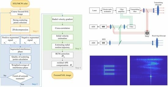
  • This article develops a motion error estimation method based on segmented interference of triangular-wave-positive and -negative frequency-modulated dechirp signals, which does not require system design changes and only requires one period of dechirp signal;
  • Innovatively proposed an initial phase estimation method based on range compression envelope cross-correlation between positive and negative frequency modulation signals;
  • An interferometric phase extraction method based on interferometric phase gradient integration is proposed, which solves the problem of interferometric phase wrapping caused by the extremely short laser wavelength.

2. Materials and Methods

In FMCW signal processing, triangular waves and sawtooth waves are two commonly used waveforms. Wang analyzed the ambiguity function of symmetric triangular waves [17], and the results showed that compared with sawtooth waves [18], triangular waves have better target resolution ability. In addition, triangular waves have been applied to target velocity and position measurement methods for a long time [19,20,21,22]. This chapter introduces triangular waves into the SAL system and proposes a new motion error compensation method based on the STLFMCW signal model.

2.1. FMCW SAL System

Inspired by the principle of triangular wave velocity measurement, this article designs the SAL system using the STLFMCW modulation method, with the basic composition structure shown in Figure 1 [23]. It mainly consists of a signal generation module, transceiver module, internal calibration module, and photoelectric detection module. The transmitted signal is a triangular linear FMCW generated by a tunable laser source. The carrier signal is generated by a seed laser source, and under the excitation of a Radio Frequency (RF) source, an electro-optic modulator is used to modulate the carrier signal into a FMCW laser signal [24]. To ensure that SAL can achieve high signal-to-noise ratio imaging of remote targets, it is necessary to generate a sufficiently high power signal. Compared to microwave radar, high-quality and high-power laser amplifiers are particularly important due to the small energy of ladar. Therefore, the Erbium-doped Fiber Amplifier (EDFA) is generally used to amplify laser signals without distortion. The amplified transmitted signal is collimated by a collimator, split by a beam splitter, and emitted by a transmitting telescope towards a far-field target. The echo reflected back by the target is received by a receiving telescope. The other path generates local oscillator light after delay, which is also split by a beam splitter. One path is mixed with the echo signal to achieve signal dechirp operation in the optical domain. The output echo dechirp signal enters the Balance Photoelectric Detector (BPD), while the other path is mixed with the split beam light of the emitted light. The generated dechirp signal is used as an internal calibration signal to enter the BPD. The internal calibration signal is used for signal quality evaluation and correction of the echo signal phase. Finally, a Digital Acquisition Card (DAC) is used to sample the dechirp signal and send the data to the computer for subsequent signal processing [25].

2.2. Analysis of Motion Error in Positive and Negative Frequency Modulation Signals of STLFMCW

This SAL system uses an STLFMCW signal, and the radial motion error generated by the non-ideal motion of the ladar will be transmitted to the echo signal. This section will analyze the motion error in the positive and negative frequency modulation signals of STLFMCW. Each period of the STLFMCW signal includes two Linear Frequency Modulation (LFM) signals with positive and negative slopes, with modulation frequencies of opposite magnitude. The positive and negative frequencies are represented as:
f = f c B r 2 + K r t r + ( 0 t r + T p / 2 ) f = f c + 3 B r 2 K r t r ( T p / 2 t r T p )
where K r denotes the modulation frequency, f c denotes the carrier frequency, B r denotes the bandwidth. t r + / t r denotes the fast time, and T p denotes PRT. The transmitted signal can be represented as:
s t + ( t r + ) = exp [ j 2 π f c t r + + j π K r t r + 2 ] s t ( t r ) = exp [ j 2 π f c t r j π K r t r 2 ]
The target echo at the range of R can be written as:
s r + ( t r + ) = exp [ j 2 π f c ( t r + 2 R c ) + j π K r ( t r + 2 R c ) 2 ] s r ( t r ) = exp [ j 2 π f c ( t r 2 R c ) j π K r ( t r 2 R c ) 2 ]
Coherently mixing the received signal with the reference signal at a reference range of R r e f to generate an echo dechirp signal, represented as:
s i f + ( t r + ) = exp [ j 4 π f c c R Δ + j 4 π c K r ( t r + 2 R r e f c ) R Δ j 4 π c 2 K r R Δ 2 ] s i f ( t r ) = exp [ j 4 π f c c R Δ j 4 π c K r ( t r 2 R r e f c ) R Δ j 4 π c 2 K r R Δ 2 ]
where R Δ = R R r e f denotes the relative reference range of the target. From the phase term in Equation (4), it can be obtained that the first term is the azimuth Doppler phase history of the signal, the second term is the linear phase about fast time, and the third term is the Residual Video Phase (RVP), which can be removed by using an RVP filter in the frequency domain. The RVP filter is represented as [23]:
H r v p ( f r ) = exp ( j π f r 2 K r )
where f r denotes the signal frequency within the fast time. After removing RVP from Equation (4), the dechirp signal shown in Equation (4) is simplified as follows:
s i f + ( t r + ) = exp [ j 4 π f c c R Δ + j 4 π c K r ( t r + 2 R r e f c ) R Δ ] s i f ( t r ) = exp [ j 4 π f c c R Δ j 4 π c K r ( t r 2 R r e f c ) R Δ ]
Then, apply Fourier transform to obtain the range-compressed results [26]:
s I F + ( f r ) = sin c [ T p ( f r f + ) ] exp [ j 4 π f c c R Δ + j π t c + ( f + f r ) j 8 π c 2 K r R r e f R Δ ] s I F ( f r ) = sin c [ T p ( f r f ) ] exp [ j 4 π f c c R Δ j π t c ( f f r ) + j 8 π c 2 K r R r e f R Δ ]
where f + = f = K r 2 R Δ c , t c + and t c represent the center times of the positive and negative frequency modulation signals of the triangular wave, respectively. From Equation (7), it can be obtained that the peak frequencies of the positive and negative frequency modulation signals after range compression are opposite to each other.
When there is a radial velocity error between the ladar platform and the target, the relative range between the ladar platform and the target is not constant. Therefore, the target range can be expressed as:
R = R 0 + Δ R
where Δ R denotes the radial motion error of the ladar platform, and the motion error Δ R can be estimated by integrating the radial velocity, that is:
Δ R ( t k ) = 0 t k v r d t a
Δ R ( t k , t r n ) = Δ R ( t k 1 ) + 0 t r n v r ( t k ) d t r
where t a denotes the azimuth slow time, V r denotes the platform radial velocity, t k denotes a certain moment, Δ R ( t k ) denotes the motion error at t k , t r n is a range certain moment, and Δ R ( t k , t r n ) is the motion error at ( t k , t r n ) . By substituting Equation (10) into Equation (6), we obtain:
s i f + ( t k , t r + ) = exp [ j 4 π f c c ( R Δ + Δ R ( t k 1 ) ) + j 4 π f c c v r ( t k ) t r + + j 4 π c K r ( t r + 2 R r e f c ) R Δ ] s i f ( t k , t r ) = exp [ j 4 π f c c ( R Δ + Δ R ( t k 1 ) ) + j 4 π f c c v r ( t k ) t r j 4 π c K r ( t r 2 R r e f c ) R Δ ]
The above equation is simplified as:
s i f + ( t k , t r + ) = exp [ j 2 π ( m 0 ( t k ) + m 1 t r + + m 2 ) ] s i f ( t k , t r ) = exp [ j 2 π ( n 0 ( t k ) + n 1 t r + n 2 ) ]
where m 0 , m 1 , and m 2 are, respectively, the slow time function term, the first-order coefficient of the fast time function, and the constant term determined by the reference range of the positive frequency modulation signal. n 0 , n 1 , and n 2 are, respectively, the slow time function term, the first-order coefficient of the fast time function, and the constant term determined by the reference range of the negative frequency modulation signal. Then, apply the Fourier transform to Equation (12) to obtain:
s I F + ( t k , f r ) = sin c [ T p ( f r f + ) ] exp [ j 2 π m 0 ( t k ) + j π t c + ( f + f r ) + m 2 ] s I F ( t k , f r ) = sin c [ T p ( f r f ) ] exp [ j 2 π n 0 ( t k ) + j π t c ( f f r ) + n 2 ] f + = f + + f d ( t k ) f = f + f d ( t k ) f d ( t k ) = 2 v r ( t k ) λ
According to Equation (13), the actual detection frequency is composed of the ideal position frequency and the Doppler frequency caused by the relative motion between the platform and the target. The schematic diagram of echo dechirp reception under the influence of radial motion error is shown in Figure 2.
In Figure 2, the red and green curves represent the instantaneous frequencies of the received signal and the reference signal, respectively. Then, the received signal and reference signal are coherently mixed to obtain the dechirp signal shown by the blue curve. The principle of coherent mixing is to multiply the received signal by the complex conjugate of the reference signal. From the blue curve, it can be seen that under the influence of radial motion error, the instantaneous frequencies of positive and negative frequency modulation signals after pulse compression are no longer opposite to each other. If radial motion errors occur on the ladar platform, in addition to positive and negative frequency modulation phases, additional phase errors will also be introduced into the dechirp signal, and this phase error is the same in positive and negative frequency modulation signals. Therefore, it is possible to consider extracting phase errors by adding the observed frequency phase of positive and negative frequency modulation signals. However, according to Equation (13), it can be observed that the phase of the positive and negative frequency modulation signals also includes a slow time function term and a constant term determined by the reference range, thereby interfering with the extraction of phase errors. Therefore, the key to this article’s research is to design algorithms to eliminate these interference terms, extract phase error information, and ultimately estimate the motion error.

2.3. A Motion Error Compensation Method Based on Segmented Interference

The positive and negative frequency modulation signals of STLFMCW are symmetrical and continuous, with strong correlation in both the time and frequency domains. Therefore, it is possible to consider using phase difference interference between positive and negative frequency modulation signals to estimate motion errors. On the basis of the established STLFMCW signal model, this section proposes a new motion error compensation strategy.

2.3.1. Segmented Interference Signal Model

Firstly, the positive and negative frequency modulation signals are segmented in the time domain. Dividing the received signal at each azimuth moment into two segmented signals with the same time width. Then, a triangular wave can be divided into four sub-signals, represented as:
s 1 + ( t k , t r ) = exp [ j 2 π ( m 0 ( t k ) + m 1 ( t r t r 1 ) + m 2 ) ] s 2 + ( t k , t r ) = exp [ j 2 π ( m 0 ( t k ) + m 1 ( t r t r 2 ) + m 2 ) ] s 1 ( t k , t r ) = exp [ j 2 π ( n 0 ( t k ) + n 1 ( t r t r 1 ) + n 2 ) ] s 2 ( t k , t r ) = exp [ j 2 π ( n 0 ( t k ) + n 1 ( t r t r 2 ) + n 2 ) ]
where s 1 + ( t r ) and s 2 + ( t r ) are segmented signals of positive frequency modulation signals with center moments of t r 1 and t r 2 , respectively; and s 1 ( t r ) and s 2 ( t r ) are segmented signals of negative frequency modulation signals with center moments of t r 1 and t r 2 , respectively. Applying Fourier transform to Equation (14), we obtain:
s 1 + ( t k , f r ) = sin c [ T p ( f r f + ) / 2 ] exp [ j 2 π ( m 0 ( t k ) + j π t r 1 ( f + f r ) + m 2 ) ] s 2 + ( t k , f r ) = sin c [ T p ( f r f + ) / 2 ] exp [ j 2 π ( m 0 ( t k ) + j π t r 2 ( f + f r ) + m 2 ) ] s 1 ( t k , f r ) = sin c [ T p ( f r f ) / 2 ] exp [ j 2 π ( n 0 ( t k ) + j π t r 1 ( f f r ) + n 2 ) ] s 2 ( t k , f r ) = sin c [ T p ( f r f ) / 2 ] exp [ j 2 π ( n 0 ( t k ) + j π t r 1 ( f f r ) + n 2 ) ]
According to Equation (15), we perform differential interference on the range frequency domain signal of positive and negative frequency modulation, and extract the phase. The extracted phase can be expressed as:
ϕ ( t k ) = arg [ s 1 + ( f r ) · s 1 ( f r ) * ] [ s 2 + ( f r ) · s 2 ( f r ) * ] * = 2 π ( t r 1 t r 2 ) ( f + f )
In Equation (16), the constant phase and the phase related to the azimuth moment are all canceled out, and the remaining phase is only determined by the observation frequency of the positive and negative frequency modulation signals. According to Equation (13), the relationship between the Doppler frequency caused by the relative motion from the platform to the target and the extracted differential interference phase is:
f d ( t k ) = ϕ ( t k ) 4 π ( t r 1 t r 2 )
The positive and negative frequency modulation signals are inevitably affected by random noise, causing the differential interference phase to be affected by random noise errors. In addition, when there are multiple point targets in a range cell, the selection of their differential interference phase is also a key issue. Therefore, this article considers selecting scattering points with a high Signal-to-Noise Ratio (SNR) and weighting the differential interference phase based on the quality of the scattering points. The formula for calculating the quality of scattering points is as follows [19,27]:
C n = E s ( l , m ) E s ( l , m ) 2 E s ( l , m )
where C n represents the contrast of the nth target, selecting a window with the size of L × M around the peak amplitude of the target; s ( l , m ) represents the matrix to be evaluated; and l and m, respectively, represent the azimuth and range indices. Therefore, the Doppler frequency at each azimuth moment is calculated by weighted average, and the expression is as follows:
f d ( t k ) = n = 1 N C n · ϕ ( t k ) 4 π ( t r 1 t r 2 ) n = 1 N C n

2.3.2. Initial Phase Estimation

In the previous section of the article, a dechirp signal model was established, and the positive and negative frequency modulation signals were segmented. The interference phase was extracted using the triangular-wave-positive and -negative frequency modulation segmented interference method, and then the Doppler frequency was extracted. The relationship between radial velocity error and Doppler frequency is shown in Equation (13); therefore, the relationship between radial velocity error and interference phase is expressed as follows:
v r ( t k ) = λ 2 ϕ ( t k ) 4 π ( t r 1 t r 2 )
In Equation (20), the magnitude of the interference phase is determined by the radial velocity, laser wavelength, and signal pulse length. The ladar emits laser signals with a wavelength of μm level; when the radial velocity is high, the interference phase is easily exceeded 2 π and phase wrapping occurs. In the case of phase wrapping, the estimation of instantaneous radial velocity is also inaccurate and differs greatly from the actual radial velocity. In addition, the method proposed in this article is to perform segmented interference on each pulse, and each pulse can only be estimated with one interference phase, so it cannot be directly unwrapped. Although the interference phase at each azimuth moment exceeds 2 π , the motion error of the actual airborne platform during flight is continuously and slowly changing, and the phase difference between adjacent azimuth moments does not exceed 2 π . Therefore, this article considers calculating the gradient of the interference phase along the azimuth direction, and then calculating the radial velocity gradient in azimuth. We just need to calculate the correct initial radial velocity, and then integrate the radial velocity gradient along the azimuth direction to accurately estimate the actual platform radial velocity error. Finally, the actual platform motion trajectory can be obtained by integrating the velocity error along the entire azimuth moment.
In response to the initial phase wrapping problem caused by the extremely short wavelength of the laser, this article adopts the method of cross-correlation between the positive and negative frequency modulation signal range compression envelopes to estimate the initial phase and then calculate the initial radial velocity. Equation (13) indicates that the Doppler frequency is caused by the relative motion between the platform and the target. The Doppler frequency caused by the relative motion between the platform and the target will change the range compression position of the target. When the motion error is large, it will cause the Doppler frequency to exceed one frequency cell, resulting in RCM in the target range compression. According to Equation (13), under the influence of radial velocity error, the peak positions of positive and negative frequency modulation signals after pulse compression are different. When the radial velocity is large, the peak position of the positive and negative frequency modulation signals after pulse compression will differ by several range cells. Constructing a pair of linear equations from the expressions of f + and f . By solving the linear equations, the Doppler frequency can be extracted, and then the radial velocity of the platform can be estimated. Therefore, this article directly obtains the relative frequency shift of the frequency spectrum of the positive and negative frequency modulation signals by cross-correlation at the first azimuth moment, and then calculates the initial radial velocity. The interference phase wrapping problem is a common phenomenon in SAL imaging due to the influence of the extremely short working wavelength of the laser. Therefore, the method proposed in this article is aimed at solving the common problem in SAL, and therefore has universality.

2.3.3. RCM Correction and Residual Azimuth Phase Error Compensation

By using the method of frequency spectrum cross-correlation between positive and negative frequency modulation signals, the initial radial velocity can be estimated, and then the radial velocity gradient can be integrated along the azimuth direction to estimate the radial velocity error v ˜ r of the platform at the entire azimuth moment. Then, construct a linear compensation function as follows:
H m ( t r ) = j 4 π v ˜ r ( t k ) t r + λ
The above filter is used to compensate for the RCM error of the positive frequency modulation signal. Then, the compensated positive frequency modulation signal can be represented as:
s 1 + ( t k , t r ) = exp [ j 2 π ( m 0 ( t k ) + j 4 π R Δ c K r t r + + m 2 ) ] s I F + ( t k , f r ) = sin c [ T p ( f r f + ) ] exp [ j 2 π m 0 ( t k ) + j π t c + ( f + f r ) + m 2 ]
After compensation by Equation (21), the observation frequency of the positive frequency modulation signal is only determined by the frequency corresponding to the target position, and the influence of Doppler frequency caused by the relative motion between the platform and the target on the RCM of the target range compression is completely eliminated. Finally, applying Fourier transform to the positive frequency modulation signal can calculate the true range of the target after eliminating motion errors.
The basic purpose of RCM correction is to correct the energy of the target to the same range cell through linear phase compensation. In Equation (22), the phase term m 0 ( t k ) of the signal regarding slow time t k includes the instantaneous slant range information between flying platform and the target in SAL two-dimensional imaging, thereby generating a secondary phase of the signal about the slow time. In SAL signal processing, a secondary compensation function, namely the azimuth match-filter function, is constructed to compensate for the azimuth secondary phase and achieve azimuth compression. However, m 0 ( t k ) contains unknown motion errors Δ R ( t k 1 ) , which disrupts the SAL azimuth ideal quadratic phase model. Therefore, after compensation by the azimuth match-filter function, there is still residual Azimuth Phase Error (APE), which affects azimuth compression and causes target azimuth defocusing. The radial velocity error estimated by Equation (15) is integrated along the azimuth according to Equations (9) and (10) to obtain the range error Δ R caused by the non-ideal motion of the flying platform. Then, constructing a compensation function to compensate for the residual APE of the echo signal, expressed as:
H a ( t a ) = exp [ j 4 π f c c Δ R ]
After compensating for the residual APE of the echo, it is multiplied by the azimuthal match-filter function to obtain the focused SAL image.

2.4. Algorithm Flow

Figure 3 shows the flowchart of motion error compensation based on STLFMCW SAL.
The first step is preprocessing, as shown in Step 1 of Figure 3. At this stage, firstly, traditional motion compensation imaging is performed using low-precision motion measurement sensors to obtain coarse-focused images. Secondly, extracting strong scattered target signals that are relatively isolated in range based on contrast so that the signal contains as much of the target’s echo energy as possible and introduces background noise as little as possible. Finally, perform two-dimensional decompression to obtain a time-domain signal containing RCM. The second step is to separate the positive and negative frequency modulation domain signals of the target, and perform segmented interference, as shown in Step 2 of Figure 3. Firstly, the positive and negative frequency modulation signals are divided into two sub-bands with the same time width in the range time domain. Performing differential interference calculation on each pair of positive and negative frequency modulation signals according to Equation (15), and extracting the Doppler phase introduced by motion error at the peak point of the range frequency spectrum. Then, based on the quality of scattering points, the differential interference phase is weighted average processing, and the interference phase at each azimuth moment is calculated through weighted average. The third step is to estimate the radial motion error, as shown in Step 3 of Figure 3. Firstly, calculate the gradient of the interference phase estimated in Step 2 along the azimuth, and then calculate the radial velocity gradient. Then, the initial phase is estimated by cross-correlation of the range-compressed envelope of the positive and negative frequency modulation signals, and then the initial radial velocity is calculated. Finally, combined with the estimated initial radial velocity, the radial velocity gradient is integrated along the azimuth to estimate the radial velocity error. The radial motion error can be obtained by integrating the estimated radial velocity error along the azimuth. The final step is motion error compensation, as shown in Step 4 of Figure 3. Firstly, a linear compensation function is constructed based on the radial motion error estimated in Step 3 to achieve RCM correction. Then, another compensation function is constructed to compensate for the residual APE in the azimuth of the signal, and finally, the focused SAL image is obtained.

3. Results and Discussion

The effectiveness of the proposed method in motion error compensation is validated through three experiments. The first and second are simulation experiments to verify the applicability of this method to different types of targets. The third experiment is a real ISAL ground imaging experiment to verify the actual effectiveness of this method.

3.1. Point Targets Simulation Experiment

This section designs a simulation experiment for three point targets, using different methods for two-dimensional imaging, and introduces three quantitative indicators to verify the effectiveness of the proposed method.

3.1.1. Experimental Setup

This section uses simulation data based on point targets to verify the effectiveness of the proposed method. The simulated SAL system parameters are shown in Table 1. A considerable amount of motion error was added in the ladar motion, which allows the target energy to span multiple range cells after pulse compression, to demonstrate the ability of this method to compensate for motion errors. Firstly, performing two-dimensional imaging on the raw data to obtain the original SAL image. Then, the original data are processed using the method proposed in this article, and compared and evaluated with the original SAL imaging result.
The simulation scene is shown in Figure 4, which consists of three point targets at different positions. Image processing was performed on the raw data without motion compensation, and the processing results are shown in Figure 5. Figure 5a shows the image after range compression. It can be seen that due to the influence of motion errors, the compressed curve has a significant curvature rather than a straight line. Figure 5b shows the SAL image obtained after azimuth match-filtering, which shows that motion errors cause severe defocusing of the three point targets.

3.1.2. Experimental Result

In this simulation experiment, the segmented interferometry was used to extract the interferometric phase of the point target echo dechirp signal, and the initial radial velocity was estimated using the cross-correlation method. Finally, the radial motion error was estimated between the ladar and the target, and the ideal error was compared with the estimation error result. Figure 6a shows the comparison between the theoretical and estimated radial velocity errors. In Figure 6a, the blue curve represents the estimated radial velocity result, and the red curve represents the ideal radial velocity. These two curves are almost identical, confirming that the algorithm mentioned in this article has high estimation accuracy. According to Equations (9) and (10), the theoretical and estimated radial velocity errors are integrated along the azimuth to obtain the motion errors caused by the non-ideal motion of the platform, as shown in Figure 6b. It can be seen that the estimated and ideal motion trajectories are almost identical. In addition, the estimation error is also plotted as shown in Figure 6c. After calculation, the maximum absolute estimation error of the algorithm proposed in this article is within 2 7 m, indicating that the estimation error is smaller than the wavelength, which verifies the effectiveness of the method proposed in this article.
Figure 7 shows the range pulse compression and azimuth-focusing results after compensation using the estimated RCM. Figure 7a shows the compensated range-compressed image. It can be seen that after motion error compensation, the target’s azimuth envelope is limited to one range cell, which verifies the effectiveness of the proposed method. Figure 7b shows the compensated two-dimensional focused image. Compared with Figure 5b, the point targets achieve good focusing results, and the imaging results of the three point targets are very close to the ideal point target.
Contour analysis is performed on these three point targets in the simulation scene, and the results are shown in Figure 8. Figure 8a,b show the contour maps of the targets before and after motion compensation, respectively. It can be seen that the point targets after compensation have achieved good focusing. In addition, Figure 9 shows the impulse spreading response of one of the point targets. This article introduces three quantitative indicators, namely Impulse Response Width (IRW), Peak Sidelobe Ratio (PSLR), and Integrated Sidelobe Ratio (ISLR) [26]. The results are listed in Table 2. The results indicate that the imaging quality under this method is very close to the ideal quality, solving the defocusing caused by RCM.

3.2. Area Target Experiment

This section designs a simulation experiment for an area target, using different methods for two-dimensional imaging. The effectiveness of the proposed method was verified by comparing the experimental results.

3.2.1. Experimental Setup

In this section, an area target simulation experiment with high SNR is designed to verify the robustness of the method proposed in this article. The essence of an area target is a region composed of several point targets with the same scattering coefficient, which are continuously distributed in the range and azimuth to form an area target [26]. Therefore, in this section of the simulation, 62 point targets are designed, and they are spaced 5 cm apart in range and 1 cm apart in azimuth. In addition, in order to facilitate the comparison of target focusing effects under different motion error estimation methods, the principle of point target spacing designed in this article is to ensure that the 3 dB main lobe width in the range and azimuth of the point targets can be separated from each other under ideal conditions after two-dimensional focusing. The simulation scene is shown in Figure 10, with a large number of points forming the shape of the letter “E’. The system parameters are consistent with the previous point target experiment.

3.2.2. Experimental Result

Firstly, the raw data are compressed by range pulse compression to obtain the original range-compressed image as shown in Figure 11a. It can be seen that due to the influence of motion errors, the curve after range compression exhibits significant curvature. In order to better verify the effectiveness of the method proposed in this article, this section will conduct comparative experiments with the conventional frequency spectral cross-correlation method [17], and verify by comparing the estimation results of RCM and motion compensation results. The results of correcting the RCM error using the cross-correlation method are shown in Figure 11b. The figure shows the processing results obtained by using 20 times upsampling. It can be seen that the pulse compression curve of the target has been basically corrected in one range cell, and the very obvious RCM has been corrected. Figure 11c shows the results of correcting the RCM error using the method proposed in the article. The pulse compression curve of the target in the figure is corrected to the same straight line.
The final two-dimensional compression imaging results are shown in Figure 12. Figure 12a shows the original two-dimensional compression results, Figure 12b shows the frequency spectral cross-correlation method results, and Figure 12c shows the imaging results based on the method proposed in this article. It can be seen that the blurring phenomenon of the targets in Figure 12a,b is clearly indistinguishable. Figure 12c can accurately estimate the residual motion error. The shape of the letter “E’ can be clearly seen in this figure, and 62 point targets can be distinguished. The imaging results are close to the ideal level.
To quantitatively evaluate the performance of the algorithm, the image entropy and the contrast are usually used to demonstrate the imaging quality. Assuming the SAL image to be evaluated is I ( l , m ) . The definition of image entropy is [6,28].
E N T = l = 1 L m = 1 M I ( l , m ) 2 E N ln I ( l , m ) 2 E N
E N = l = 1 L m = 1 M I ( l , m ) 2
where E N is the total energy of the SAL image. The entropy is inversely proportional to target focusing effect. The definition of SAL image contrast is:
C = E I ( l , m ) E I ( l , m ) 2 E I ( l , m )
The contrast is directly proportional to the focusing effect of the target. This section calculated the image entropy and contrast of Figure 12, as shown in Table 3.
The entropy of the defocused SAL image in Figure 12a is 11.4919, and the contrast is 0.2375. After spectral cross-correlation processing, the entropy value of the SAL image is 11.4081, and the contrast is 0.3146. Compared with Figure 12a, after motion error compensation using the cross-correlation method, the target achieved a certain focusing effect, and the target energy was also enhanced after focusing. However, the letter “E” still cannot be recognized. This indicates that the cross-correlation method cannot accurately estimate residual motion errors in severely defocused SAL images. After processing with the method proposed in this article, the entropy value of the SAL image is 11.3471, and the contrast is 0.3433. Compared with the previous two sets of data, the entropy value is greatly reduced, and the contrast is significantly improved. Compared with Figure 12a,b, the focus quality of the target has been greatly improved, and the letter “E” can be clearly identified. The comparison of the above experiments proves that the proposed method can greatly improve the quality of SAL images.

3.3. Ground ISAL Experiment

Considering that the motion error compensation method is applicable to different SAL imaging modes, in order to facilitate experimental operability, this article will use an ISAL ground experiment to verify the effectiveness of the proposed method in real scenes.

3.3.1. Experimental Setup

ISAL operates in a fixed ladar mode for target movement [29], and its imaging principle is similar to the spotlight mode SAL. It is often applied in the field of ground-based ISAL for observing spatial targets. The ISAL observation geometry is shown in Figure 13, which shows the motion decomposition of a target relative to the ladar.
LOS denotes ladar line of sight, the motion of the target is equivalent to revolve, translation, and rotation; θ ( t ) denotes equivalent rotation angle; d ( t ) denotes equivalent translation distance; and q ( t ) denotes equivalent revolve angle. When there is radial motion of the target relative to the ladar, it not only does not contribute to the azimuthal focusing, but also causes the target pulse compressed curve to migrate across range cells, deteriorating the two-dimensional focusing effect of the target. In addition, due to the fact that laser waves are always smaller than microwave wavelengths, system vibrations, and atmospheric disturbances may cause the compressed signal to migrate across range cells.
The real experiment adopts the inverse synthetic aperture ladar system provided by the Chinese Academy of Sciences. The appearance, experimental scene, and optical photos of the experimental target of the ISAL system are shown in Figure 14. The ladar system structure is shown in Figure 14a. The optical transceiver lens is suspended on the rack, and the laser beam is tilted at a 45 angle and emitted from the laser transceiver lens. It is horizontally irradiated towards the far field through a large reflector. Figure 14b shows the scene of the ISAL far-field imaging experiment in the laboratory, where the laser emitted by the ladar is irradiated onto a cooperative target at a distance of 4.3 km in the far-field. The cooperative target is a single retro-reflector and a broken line shape composed of high reflectivity bars, as shown in Figure 14c. The size of the broken line is indicated by a yellow arrow in Figure 14c, and the red-framed target is a retro-reflector target with a diameter of 1.2 cm.
The system parameters are listed in Table 4. The STLFMCW signal with a 32 μs of PRT is transmitted, the sampling frequency is 150 MHz, and the beamwidth of the SAL system antenna used is 120 μrad × 30 μrad.

3.3.2. Experimental Result

In the simulation experiments, two isolated data for positive and negative frequency modulation echo signals are designed, respectively. However, in the practical experiment, when processing the received echoes, a continuous set of triangular dechirp signals is received, and the positive and negative frequency modulation components must be separated from this dechirp signal in order to perform subsequent segmented interference processing. Firstly, the time–frequency analysis is performed on the echo dechirp signal and Short Time Fourier Transform (STFT) is performed on a periodic signal to calculate the instantaneous frequency, as shown in Figure 15a. From Figure 15a, it can be observed that, unlike the ideal triangular dechirp signal in Figure 2, the instantaneous frequency of the actual dechirp signal at time 0 is not 0. In this case, it is difficult to separate the positive and negative frequency modulation components from the dechirp signal. Therefore, the method of performing circular shift is adopted on the echo signal in the range time domain so that the instantaneous frequency of the signal at time 0 is 0. STFT is performed on the signal after circular shift to calculate the time–frequency relationship, as shown in Figure 15b. From Figure 15b, it can be seen that the positive and negative frequency modulation components of the dechirp signal correspond to the front and rear half triangular wave signal, respectively. Therefore, we intercept the first half of the echo signal as a positive frequency-modulated signal, and the second half of the echo signal as a negative frequency-modulated signal, ultimately separating the positive and negative frequency-modulated components in STLFMCW. The corresponding echoes are shown in Figure 15c and Figure 15d, respectively.
According to Figure 13, it can be observed that the cooperative target consists of a strong point target and an area target. This section first performs range compression on the original data, as shown in Figure 16a. It can be observed that the brighter curve in the lower part of the figure is the echo data of the retro-reflector, whose signal strength is much greater than that of the broken line in the upper part. From Figure 16a, it can be seen that the motion error caused by the relative radial motion of the target to the ladar causes the pulse pressure curve of the retro-reflector to bend. In addition, due to the influence of atmospheric turbulence and ladar beam vibration, the intensity of the target echo signal is uneven, and even leads to blurred imaging of the signal in range. The radial motion errors between the target and the platform will affect the entire imaging plane of the target illuminated by the laser beam. Although the positions of these targets are different, they will all be accompanied by Doppler frequencies introduced by radial motion errors. Therefore, motion error estimation can be performed on the echo data of the retro-reflector and the estimated motion error can be compensated for throughout the entire imaging scene. To better demonstrate the effectiveness of the proposed method, this section will also conduct comparative experiments with the conventional cross-correlation method.
The result of correcting the RCM error using the cross-correlation method in this section is shown in Figure 16b. The figure shows the processing results obtained by 20 times upsampling. It can be seen that the significant RCM in the target’s pulse compression curve has been corrected, but there is still curvature, and the target’s energy has not been fully concentrated in the same range cell. Figure 16c shows the results of correcting the RCM using the method proposed in this article. It can be seen that the pulse compression curve of the target in the figure has been corrected to the same range cell, indicating that the motion error has been well eliminated and the energy of the target echo signal has been concentrated. Compared with the cross-correlation method, the proposed method estimates higher accuracy radial motion error by using segmented interferometry to extract phase.
This section presents the radial velocity error and radial motion error estimated by the cross-correlation method and the proposed method in Figure 17. Figure 17a compares the radial velocity errors estimated by the two methods, with the red curve representing the cross-correlation method and the green curve representing the estimation results of the proposed method in this article. The estimated radial motion error is obtained by integrating the estimated radial velocity error along the azimuth, as shown in Figure 17b. By comparing the estimation results of the two methods, it is not difficult to find that using only the method of cross-correlation from the amplitude of positive and negative frequency modulation pulse compression signals makes it difficult to accurately estimate the offset of the range frequency spectrum caused by the motion error. However, it can estimate the approximate trend of the target motion trajectory and correct most of the RCM. This article uses positive and negative frequency modulation segmented interference to extract the interference phase, calculates the phase gradient, and then uses the cross-correlation method to obtain the initial phase. The Doppler phase is calculated by integrating the phase gradient, and then the radial motion velocity and radial motion error of the target are calculated. By comparing the estimation results of the proposed method with those of the cross-correlation method, it can be seen that the amplitude scope of the estimated values is greater than that of the cross-correlation method, proving that the interference phase extracted by the proposed method contains richer motion error information.
The final two-dimensional compression imaging results are shown in Figure 18. Figure 18a shows the two-dimensional compression results of the original data. Figure 18b,c, respectively, show the comparison results between the cross-correlation method and the proposed method for correcting the motion error. It is easy to see that the scene target blur phenomenon is obvious in Figure 18a,b, while Figure 18c indicates that the proposed method can accurately estimate residual motion errors.
To quantitatively evaluate the performance of the algorithm, the image entropy and contrast of images were calculated under different motion compensation algorithms, as shown in Table 5. In Table 5, the method proposed in this article has the lowest image entropy and the highest contrast. At the same time, we also compared the azimuth and range point extension responses of the retro-reflector and plotted them in Figure 19. Finally, the IRW, PSLR, and ISLR of the retro-reflector were calculated, as shown in Table 6.
In Figure 19, the blue curve represents the spectral cross-correlation method, and the red curve represents the estimation results of the proposed method. There is no significant difference between the two range-oriented slices in Figure 19b, but in Figure 19a, it is easy to see that there is a significant difference in the azimuth-oriented slices. Under the proposed method, the azimuth direction of the signal is well focused, and the quality parameters under the methods proposed in Table 6 are better than those of the cross-correlation method. The above results indicate that the proposed method has significant advantages over the cross-correlation method.

4. Conclusions

In FMCW SAL imaging, the radial motion error between the ladar platform and the target can cause RCM of the target, seriously affecting the azimuth-focusing result. A SAL motion compensation method based on STLFMCW segmented interference is proposed. Firstly, the influence of radial motion error on the range pulse compression of STLFMCW SAL signals was derived. Based on the radial motion error model, the positive and negative frequency modulation signals were segmented, and the segmented interference method was used to extract Doppler frequency. Based on the relationship between radial velocity error and Doppler frequency, the radial velocity gradient along the azimuth was calculated. Then, in response to the initial phase wrapping problem, the method of cross-correlation between positive and negative frequency modulation signals was used to accurately estimate the initial phase, and then calculate the initial radial velocity error. Finally, using the estimated initial radial velocity, the radial velocity gradient is integrated along the azimuth to obtain the platform motion trajectory. This article verifies through simulation experiments on point and area targets, as well as real-ground ISAL experiments, that this method can eliminate the influence of radial motion errors on two-dimensional imaging, and achieve good focus in the azimuth of the target. Compared with traditional motion error compensation methods, this method does not require changes in the hardware design of the ladar system and only uses a one-period STLFMCW signal, and is of great significance for high-resolution FMCW SAL imaging.
However, when there is a serious motion error with time-varying acceleration, it not only causes RCM, but also introduces higher-order errors, which will most seriously affect the range pulse compression results. Due to the limited accuracy of interferometric phase estimation for high-order errors, the method proposed in this article may not be effective in improving range pulse compression results. Therefore, we will consider the impact of high-order time-varying motion errors on range and azimuth focusing in future research, and improve the algorithm to make it suitable for echo signals under the influence of such motion errors.

Author Contributions

Conceptualization, B.W., M.X. and R.S.; investigation, R.S. and W.L.; software, R.S. and W.L.; writing—original draft preparation, R.S.; writing—review and editing, R.S., Q.D. and Y.W. All authors have read and agreed to the published version of the manuscript.

Funding

This research received no external funding.

Data Availability Statement

No new data were created or analyzed in this study. Data sharing is not applicable to this article.

Acknowledgments

The authors thank the staff of the National Key Laboratory of Microwave Imaging Technology, Aerospace Information Research Institute, Chinese Academy of Sciences, for their valuable conversations and comments.

Conflicts of Interest

The authors declare no conflicts of interest.

References

  1. Bashkansky, M.; Lucke, R.L.; Funk, E.E.; Reintjes, J.F.; Rickard, L.J. Synthetic aperture imaging at 1.5 um: Laboratory demonstration and potential application to planet surface studies. In Proceedings of the Highly Innovative Space Telescope Concepts, Waikoloa, HI, USA, 22–23 August 2002; SPIE: Bellingham, WA, USA, 2002; Volume 4849, pp. 48–56. [Google Scholar]
  2. Abdukirim, A.; Ren, Y.; Tao, Z.; Liu, S.; Li, Y.; Deng, H.; Rao, R. Effects of Atmospheric Coherent Time on Inverse Synthetic Aperture Ladar Imaging through Atmospheric Turbulence. Remote Sens. 2023, 15, 2883. [Google Scholar] [CrossRef]
  3. Karr, T.J. Resolution of synthetic-aperture imaging through turbulence. JOSA A 2003, 20, 1067–1083. [Google Scholar] [CrossRef]
  4. Turbide, S.; Marchese, L.; Terroux, M.; Bergeron, A. Synthetic aperture lidar as a future tool for earth observation. In Proceedings of the International Conference on Space Optics—ICSO, Tenerife, Spain, 6–10 October 2014; SPIE: Bellingham, WA, USA, 2017; Volume 10563, pp. 1115–1122. [Google Scholar]
  5. Nelson, R.; Oderwald, R.; Gregoire, T.G. Separating the ground and airborne laser sampling phases to estimate tropical forest basal area, volume, and biomass. Remote Sens. Environ. 1997, 60, 311–326. [Google Scholar] [CrossRef]
  6. Lv, Y.; Wu, Y.; Wang, H.; Qiu, L.; Jiang, J.; Sun, Y. An Inverse Synthetic Aperture Ladar Imaging Algorithm of Maneuvering Target Based on Integral Cubic Phase Function-Fractional Fourier Transform. Electronics 2018, 7, 148. [Google Scholar] [CrossRef]
  7. Guo, L.; Yin, H.; Zeng, X.; Xing, M.; Tang, Y. Analysis of airborne synthetic aperture ladar imaging with platform vibration. Optik 2017, 140, 171–177. [Google Scholar] [CrossRef]
  8. Bashkansky, M.; Lucke, R.L.; Funk, E.; Rickard, L.; Reintjes, J. Two-dimensional synthetic aperture imaging in the optical domain. Opt. Lett. 2002, 27, 1983–1985. [Google Scholar] [CrossRef] [PubMed]
  9. Karr, T.J. Atmospheric Phase Error in Coherent Laser Radar. IEEE Trans. Antennas Propag. 2007, 55, 1122–1133. [Google Scholar] [CrossRef]
  10. Depoy, R.S.; Shaw, A.K. Algorithm to overcome atmospheric phase errors in SAL data. Appl. Opt. 2020, 59, 140–150. [Google Scholar] [CrossRef] [PubMed]
  11. Hua, Z.; Li, H.; Gu, Y. Atmosphere turbulence phase compensation in synthetic aperture ladar data processing. In Proceedings of the MIPPR 2007: Multispectral Image Processing, Wuhan, China, 15–17 November 2007; SPIE: Bellingham, WA, USA, 2007; Volume 6787, pp. 560–566. [Google Scholar]
  12. Lv, Y.k.; Wu, Y.h. Development and key technologies of synthetic aperture ladar imaging. Laser Optoelectron. Prog. 2017, 54, 43–59. [Google Scholar]
  13. Gatt, P.; Jacob, D.; Bradford, B.; Marron, J.; Krause, B. Performance bounds of the phase gradient autofocus algorithm for synthetic aperture ladar. In Proceedings of the Laser Radar Technology and Applications XIV, Orlando, FL, USA, 15–16 April 2009; SPIE: Bellingham, WA, USA, 2009; Volume 7323, pp. 187–195. [Google Scholar]
  14. Attia, E.H. Data-adaptive motion compensation for synthetic aperture LADAR. In Proceedings of the 2004 IEEE Aerospace Conference Proceedings, Big Sky, MT, USA, 6–13 March 2004; IEEE Cat. No. 04TH8720. IEEE: New York, NY, USA, 2004; Volume 3, pp. 1782–1787. [Google Scholar]
  15. Stappaerts, E.A.; Scharlemann, E.T. Differential synthetic aperture ladar. Opt. Lett. 2005, 30, 2385–2387. [Google Scholar] [CrossRef]
  16. Ma, M.; Li, D.; Du, J. Imaging of airborne synthetic aperture ladar under platform vibration condition. J. Radars 2014, 3, 591. [Google Scholar] [CrossRef]
  17. Wang, S.; Wang, B.; Xiang, M.; Sun, X.; Xu, W.; Wu, Y. Synthetic aperture ladar motion compensation method based on symmetrical triangular linear frequency modulation continuous wave. Opt. Commun. 2020, 471, 125901. [Google Scholar] [CrossRef]
  18. Stove, A.G. Linear FMCW radar techniques. IEE Proc. F (Radar Signal Process.) 1992, 193, 343–350. [Google Scholar] [CrossRef]
  19. Pierrottet, D.; Amzajerdian, F.; Petway, L.; Barnes, B.; Lockard, G.; Rubio, M. Linear FMCW laser radar for precision range and vector velocity measurements. MRS Online Proc. Libr. (OPL) 2008, 1076, 1076-K04. [Google Scholar] [CrossRef]
  20. Amzajerdian, F.; Pierrottet, D.; Petway, L.; Hines, G.; Roback, V. Lidar systems for precision navigation and safe landing on planetary bodies. In Proceedings of the International Symposium on Photoelectronic Detection and Imaging 2011: Laser Sensing and Imaging; and Biological and Medical Applications of Photonics Sensing and Imaging, Beijing, China, 24–26 May 2011; SPIE: Bellingham, WA, USA, 2011; Volume 8192, pp. 27–33. [Google Scholar]
  21. Amzajerdian, F.; Hines, G.D.; Pierrottet, D.F.; Barnes, B.W.; Petway, L.B.; Carson III, J.M. Demonstration of coherent Doppler lidar for navigation in GPS-denied environments. In Proceedings of the Laser Radar Technology and Applications XXII, Anaheim, CA, USA, 11–12 April 2017; SPIE: Bellingham, WA, USA, 2017; Volume 10191, p. 1019102. [Google Scholar]
  22. Pierrottet, D.; Amzajerdian, F.; Petway, L.; Barnes, B.; Lockard, G.; Hines, G. Navigation Doppler Lidar sensor for precision altitude and vector velocity measurements: Flight test results. In Proceedings of the Sensors and Systems for Space Applications IV, Orlando, FL, USA, 25–26 April 2011; SPIE: Bellingham, WA, USA, 2011; Volume 8044, pp. 240–250. [Google Scholar]
  23. Bingnan, W.; Juanying, Z.; Wei, L.; Ruihua, S.; Maosheng, X.; Yu, Z.; Jianjun, J. Array Synthetic Aperture Ladar with High Spatial Resolution Technology. J. Radars 2022, 11, 1110–1118. [Google Scholar]
  24. Mengmeng, X.; Yu, Z.; Jianfeng, S.; Zhiyong, L.; Chenzhe, L.; Hongyu, H.; Yuexin, L. Generation of linear frequency modulation laser source with broadband narrow linewidth using optical phase modulator. Infrared Laser Eng. 2020, 49, 0205004. [Google Scholar] [CrossRef]
  25. Li, G.; Wang, N.; Wang, R.; Zhang, K.; Wu, Y. Imaging method for airborne SAL data. Electron. Lett. 2017, 53, 351–353. [Google Scholar] [CrossRef]
  26. Cumming, I.G.; Wong, F.H. Digital processing of synthetic aperture radar data. Artech House 2005, 1, 108–110. [Google Scholar]
  27. Berizzi, F.; Corsini, G.; Diani, M.; Veltroni, M. Autofocus of wide azimuth angle SAR images by contrast optimisation. In Proceedings of the IGARSS’96. 1996 International Geoscience and Remote Sensing Symposium, Lincoln, NE, USA, 31–31 May 1996; IEEE: New York, NY, USA, 1996; Volume 2, pp. 1230–1232. [Google Scholar]
  28. Yakun, L.; Yanhong, W.; Hongyan, W.; Shiqiang, S. Phase errors compensation algorithm of inverse synthetic aperture ladar based on CS-Fmea. In Proceedings of the 2017 3rd IEEE International Conference on Computer and Communications (ICCC), Chengdu, China, 13–16 December 2017; IEEE: New York, NY, USA, 2017; pp. 1313–1317. [Google Scholar]
  29. Turbide, S.; Marchese, L.; Terroux, M.; Bergeron, A. Investigation of synthetic aperture ladar for land surveillance applications. In Proceedings of the Electro-Optical Remote Sensing, Photonic Technologies, and Applications VII; and Military Applications in Hyperspectral Imaging and High Spatial Resolution Sensing, Dresden, Germany, 24–26 September 2013; SPIE: Bellingham, WA, USA, 2013; Volume 8897, pp. 68–75. [Google Scholar]
Figure 1. The basic composition structure of FMCW SAL system. ADC: Analog-to-Digital Converter.
Remotesensing 16 00793 g001
Figure 2. The instantaneous frequency of STLFMCW and dechirp signal.
Remotesensing 16 00793 g002
Figure 3. Process flow of the proposed motion compensation method.
Remotesensing 16 00793 g003
Figure 4. Simulation scene.
Remotesensing 16 00793 g004
Figure 5. Image processing results without motion compensation. (a) Range-compressed image. (b) SAL image.
Remotesensing 16 00793 g005
Figure 6. Comparison between the theoretical and estimated results. (a) Velocity comparison. (b) Motion error comparison. (c) Estimation errors in meters.
Remotesensing 16 00793 g006
Figure 7. Image processing results after motion compensation. (a) Range-compressed image. (b) SAL image.
Remotesensing 16 00793 g007
Figure 8. Contour map of the point targets. (a) No motion compensation. (b) Compensation with proposed method.
Remotesensing 16 00793 g008
Figure 9. Impulse spreading response. (a) Range profile and (b) Azimuth profile of the focused image.
Remotesensing 16 00793 g009
Figure 10. Simulation scene.
Remotesensing 16 00793 g010
Figure 11. Range pulse compression. (a) Original. (b) Cross-correlation. (c) Proposed method.
Remotesensing 16 00793 g011
Figure 12. Imaging results based on the (a) no motion compensation method, (b) cross-correlation method, and (c) the proposed method.
Remotesensing 16 00793 g012
Figure 13. ISAL observation geometry model.
Remotesensing 16 00793 g013
Figure 14. The platform of the ISAL system. (a) Photograph of ISAL system. (b) Imaging scene. (c) Target optical photo.
Remotesensing 16 00793 g014
Figure 15. Extraction of positive and negative frequency modulation signals of the echo. (a) STFT of original echo. (b) STFT after circular shift. (c) Positive frequency modulation. (d) Negative frequency modulation signal.
Remotesensing 16 00793 g015
Figure 16. The range-compressed images with different correction methods. (a) Original. (b) Cross-correlation. (c) Proposed method.
Remotesensing 16 00793 g016
Figure 17. Estimated results comparison. (a) Estimated radial velocity errors. (b) Estimated motion errors.
Remotesensing 16 00793 g017
Figure 18. Imaging results. (a) Original. (b) Cross-correlation. (c) Proposed method.
Remotesensing 16 00793 g018
Figure 19. Comparison of the pulse-response curves in the azimuth (a) and range directions (b).
Remotesensing 16 00793 g019
Table 1. Parameters of the simulated SAL system.
Waveform of LadarLaser WavelengthBandwidthPRTVelocityPlatform Height
STLFMCW1.55 μm5 GHz16 μs60 m/s3000 m
Table 2. Quality assessment.
IRW (m)PSLR (dB)ISLR (dB)
Range0.030−13.23−12.26
Azimuth0.006−12.49−11.98
Table 3. Performance comparisons of images.
OriginalCross-CorrelationProposed Method
Entropy11.491911.408111.3471
Contrast0.23750.31460.3433
Table 4. Performance comparisons of images.
ParametersValues
Waveform of LadarTriangular FMCW
Laser Wavelength1.55 μm
Bandwidth5 GHz
PRT32 μs
Operating Range4350 m
Incident Angle45°
Range Cell0.03 m
Azimuth Cell0.0001 m
Reference Range4339.5 m
Beam Width120 μrad × 30 μrad
Table 5. Performance comparisons of images.
OriginalCross-CorrelationProposed Method
Entropy13.043412.023911.9251
Contrast0.32070.33000.4100
Table 6. Quality assessment.
IRW (m)PSLR (dB)ISLR (dB)
Cross-CorrelationProposedCross-CorrelationProposedCross-CorrelationProposed
Range0.0300.030−10.36−14.00−9.92−13.20
Azimuth0.00800.0078−5.01−13.77−3.86−12.78
Disclaimer/Publisher’s Note: The statements, opinions and data contained in all publications are solely those of the individual author(s) and contributor(s) and not of MDPI and/or the editor(s). MDPI and/or the editor(s) disclaim responsibility for any injury to people or property resulting from any ideas, methods, instructions or products referred to in the content.

