Article

Satellite and Ground Based Thermal Observation of the 2014 Effusive Eruption at Stromboli Volcano

1
Institute of Geophysics, Center for Earth System Research and Sustainability, University of Hamburg, Bundesstraße 55, Hamburg D-20146, Germany
2
German Aerospace Center, Optical Information Systems, Rutherfordstraße 2, Berlin D-12489, Germany
*
Author to whom correspondence should be addressed.
Remote Sens. 2015, 7(12), 17190-17211; https://0-doi-org.brum.beds.ac.uk/10.3390/rs71215876
Submission received: 6 September 2015 / Revised: 3 December 2015 / Accepted: 8 December 2015 / Published: 18 December 2015
(This article belongs to the Special Issue Volcano Remote Sensing)

Abstract

:
As specifically designed platforms are still unavailable at this point in time, lava flows are usually monitored remotely with the use of meteorological satellites. Generally, meteorological satellites have a low spatial resolution, which leads to uncertain results. This paper presents the first long term satellite monitoring of active lava flows on Stromboli volcano (August–November 2014) at high spatial resolution (160 m) and relatively high temporal resolution (~3 days). These data were retrieved by the small satellite Technology Experiment Carrier-1 (TET-1), which was developed and built by the German Aerospace Center (DLR). The satellite instrument is dedicated to high temperature event monitoring. The satellite observations were accompanied by field observations conducted by thermal cameras. These provided short time lava flow dynamics and validation for satellite data. TET-1 retrieved 27 datasets over Stromboli during its effusive activity. Using the radiant density approach, TET-1 data were used to calibrate the MODVOLC data and estimate the time averaged lava discharge rate. With a mean output rate of 0.87 m3/s during the three-month-long eruption, we estimate the total erupted volume to be 7.4 × 10⁶ m3.

Graphical Abstract

1. Introduction

Stromboli is one of the Aeolian Islands that build the volcanic arc north of Sicily (Italy). The island contains an active volcano with the same name. Its Strombolian eruptions [1,2] are often visible from the surrounding sea, which lead to the island’s nickname “Lighthouse of the Mediterranean”. The volcano’s typical activity is characterized by regular explosions that eject particles ~100 m above the crater terrace a couple of times per hour. Continuous effusive activity is uncommon for Stromboli. During the last decades, only three major effusive episodes were recorded: 1985/86 [3], 2002/03 [4,5] and 2007 [6,7,8]. The effusive activity presents no direct hazard to the island’s inhabitants. However, the effusive activity has often been followed by paroxysmal phases which might cause the partial collapse of the Sciara del Fuoco (part of the north slope of the volcano). Sciara del Fuoco could also collapse due to a submarine landslide at the start of an effusive eruption; this was the case during the 2002/2003 eruption, which also produced a tsunami [9,10]. In other words, the effusive activity at Stromboli is an exceptional activity that can be a precursor of a major hazard in the broader area.
A new effusive activity period at Stromboli started on 6 August 2014. This event had been preceded by two months of increased Strombolian activity and several lava overflows from its different craters [11,12]. Lava flows extended down the Sciara del Fuoco from a fracture 650 m a.s.l.. The effusive period lasted until 13 November 2014. Thermal observations of this event allowed us to estimate the time averaged lava discharge rate. The thermal data were retrieved by the Moderate Resolution Imaging Spectroradiometer (MODIS) and the small TET-1 satellite (German abbreviation for “Technologie-Erprobungsträger 1” meaning Technology Experiment Carrier). This was the first time a small and low cost satellite provided a long term satellite monitoring of active lava flows at high spatial resolution (160 m) and a relatively high temporal resolution (~3 days, sometimes even two images per day).
Prior to the presentation of the satellite and field data processing in Section 3, a brief review of techniques for thermal observations of active volcanoes is given in Section 2. Volcanic radiant power and time averaged lava discharge rates derived from satellite observations are presented in Section 4. These are followed by a discussion focusing on the comparison of TET-1 data to other satellite data and field observations.

2. Thermal Observations of Active Volcanoes

An active lava flow emits more radiation than its surroundings and variations in the amount of radiated heat reveal a lot about the processes that take place within these flows. The temperature within a lava flow ranges between 400 and 1200 K [13]. According to Wien’s displacement law, the peak emission of the radiance for blackbody surfaces at temperatures 600–1000 K is between 3 and 5 μm (i.e., in the medium infrared (MIR)). For a temperature of 300 K (typical surface temperature of the Earth), which is the expected temperature to be measured by earth orbiting radiometers, the peak of the radiance emission is located at approximately 10 μm (i.e., in the thermal infrared spectrum (TIR)).
Satellite instruments and field thermal cameras can measure spectral radiance at different wavelengths. If the measured surface is isothermal on the pixel scale the spectral radiance can easily be converted to a temperature (Planck’s law). However, the surface of an active volcano is composed of lava crust of different ages, possibly fresh lava, vegetation, water, etc. Considering Wien’s law, it is also possible to detect and quantify volcanic thermal anomalies even if they do not cover an entire satellite pixel. The detected thermal anomalies are usually quantified by their temperature, area, volcanic radiant power (VRP), or time averaged lava discharge rate (TADR) [14,15,16,17,18,19,20,21,22,23,24]. The uncertainty of single measured spectral radiances depends on numerous factors such as different sensor’s point spread function and spectral response functions, different time of overpass, orbit geometry, and spatial resolution [25,26].

2.1. Characteristics of Instruments Suitable for Observing Volcanic Thermal Anomalies

The most important source of uncertainties in thermal monitoring of active volcanoes from space stems from the lack of dedicated satellite instruments. A perfect instrument dedicated to monitoring thermal anomalies should have the following characteristics:
  • high spatial resolution (width of an average lava flow <20 m),
  • short revisit time (<15 min),
  • numerous spectral channels, or at least an appropriate combination of channels [27],
  • high radiometric accuracy (<0.1 K), and
  • automatic adjustment of gain settings, i.e., being able to observe high and low temperature events using the same sensor.
Considering the currently available technology, such instruments are not available. This leads to compromises between spatial and temporal resolution—if the data were available at high temporal resolution (from geostationary instruments), it is impossible to provide high spatial resolution data. The most promising solution seems to be a constellation of small satellites, as proposed by ESA [28], for they can provide data at high spatial resolution and provide a short revisit time as there is a high number of satellites in the constellation.
In addition, it is difficult to provide narrow spectral channels at high radiometric accuracy for monitoring high and low temperatures at the same time. Instruments designed for meteorological applications are usually used in remote sensing of volcanic thermal anomalies. These instruments also contain a MIR channel, which provides crucial data for monitoring active volcanoes. However, the settings of meteorological instruments are optimized for monitoring low temperatures, which results in often saturated data over active volcanoes. The saturation level depends on the temperature of the observed anomaly and its size, as well as on the instrument’s settings. Taking 1500 K as the upper limit for volcanic thermal anomalies, the saturation of the instrument’s signal depends on the size of the anomaly. This means that instruments with coarser spatial resolution are less prone to saturation than high resolution instruments. However, high resolution instruments are necessary in order to observe the exact position of the anomaly and precisely quantify its amplitude.
The currently operational instruments suitable for monitoring volcanic thermal anomalies with spatial resolution of no more than 100 m are: (1) the Operational Land Imager (OLI) accompanied by the Thermal Infrared Sensor (TIRS) on-board Landsat-8; and (2) the Advanced Spaceborne Thermal Emission and Reflection Radiometer (ASTER) on-board Terra satellite. The latter has a malfunction in its short-wave infrared channels since spring 2008, which limits its use for the quantification of thermal anomalies. An alternative is represented by the Visible Infrared Imaging Radiometer Suite (VIIRS) on board the Suomi National Polar-orbiting Partnership satellite, which provides a suitable spectral channel (VIIRS I4) also at 375 m spatial resolution, but this channel becomes saturated already at 367 K [29]. Another option could be the Chinese small satellite HJ-1B (spatial resolution of 150 m in the MIR channel), however its data are not available in an open access web archive.

2.2. TET-1

The volcanological community has partially overcome the gap between the available meteorological satellites and its requirements with the small satellite TET-1. TET-1 is the first satellite within the FireBird constellation [30]. This consists of two small satellites that are predominantly dedicated to investigating high temperature events. They were built and are operated by the German Aerospace Center (DLR). The constellation is designed on the basis of the Bi-spectral Infra-Red Detection (BIRD) satellite [31]. TET-1 was launched on 12 June 2012. The second satellite in the constellation, the Bi-spectral Infrared Optical System (BIROS), is scheduled to be launched in spring 2016. Together they will provide one dataset per day. BIROS is still not operational, but its basic characteristics are almost identical to TET-1 (Table 1; for further details on the TET-1 mission see Lorenz et al. [30] and Fischer et al. [32]). We have ascertained that FireBird satellites have one important advantage over other satellite instruments—their on-board processing allows repeated acquisition over the same area within a few microseconds, thus preventing data saturation. Another specific characteristic of the FireBird satellites is represented by the staggered line arrays in their pushbroom cameras [33], which results in a step in its spatial sampling half the size of the effective pixel size (Table 1).
Table 1. Main characteristics of TET-1 instruments [32].
Parameter1 VIS Camera2 IR Cameras
Wavelength460–560 nm
565–725 nm
790–930 nm
3.4–4.2 μm
8.5–9.3 μm
Quantization14 bit
Swath width192 km162 km
Spatial resolution40 m320 m
Ground sampling distance40 m160 m
FireBird retrievals can be ordered at DLR [34]. Currently this procedure is semi-automatic and it takes approximately three days from when the data are ordered and the first retrieval. However, the 2014 Stromboli eruption started in the middle of the summer vacation season and the ordering procedure was longer at that time, thus the first data were retrieved only three weeks after the eruption started.

3. TET-1 Data Processing Chain

The processing chain of TET-1 data consist of the steps presented in Figure 1. These steps are described in greater detail in the following subsections. The processing of MODIS and field data is similar, but as MODIS data originates from the MODVOLC database [21,35], it does not undergo exactly the same processing chain.
Figure 1. Basic scheme of the TET-1 processing chain.
Remotesensing 07 15876 g001

3.1. Pre-Processing

It is necessary to correct data for atmospheric effects. In our study, we applied MODTRAN [36] atmospheric transmittance and up-welling irradiance based on a mid-latitude summer model. The upwelling irradiance is a significant source of errors in the TIR band, but does not provide such significant errors at shorter wavelengths [37]. The reflected irradiance was also ignored, which is reasonable over hot bodies [37]. In addition to the atmospheric effects, the data were also corrected for emissivity. For Stromboli, a grey body assumption was applied, with a flat emissivity of 0.95 [4,5].
Data de-convolution is an important step in pre-processing. This is important in the case of a sub-pixel object that acts as an anomaly in a relatively homogeneous background—for instance a lava flow observed in a MIR band. In this case, the signal may be dispersed over several pixels although a typical lava flow is no more than a pixel wide in most satellite instruments. This effect is a result of the imperfect point spread function of the optics on satellite instruments [26,38]. In the case of TET-1, this is a very important step as its spatial sampling is 160 m, but the effective pixel size is twice as large (Table 1). This results in a somewhat blurred image. In TET-1 this effect is most significant in the MIR channel, thus only the data for this channel were de-convoluted using the Richardson–Lucy algorithm [39,40]. Various iterations were tested using our data, and the differences in the maximum radiance values varied by 3% between five and 100 iterations. When a higher number of iterations was used, more artifacts became visible around the lava flow, thus the algorithm was run with only five iterations. The de-convolution increased the maximum MIR radiance values in an image from about 3.5 to 4.5 W/m2/sr/μm.

3.2. Co-Registration of MIR and TIR Channels

TET-1 MIR and TIR channels are acquired with separate cameras, which causes uncertainties in inter-channel georeferencing, as the MIR and TIR pixels may not be optimally co-registered. The same problem arises for data acquired with a third camera in the visible (red and green channel) and near infrared spectrum (in the continuation abbreviated to VNIR; these three channels have 40 m spatial resolution).
As clouds may cover a large fraction of the acquired images, they play a pivotal role in georeferencing new images. However, clouds have different spectral characteristics at different wavelengths. In the MIR spectrum, the clouds appear to be bright during the daytime, but dark during the night. Clouds always appear dark in the TIR spectrum. The gradient between neighboring pixels is used to overcome the wavelength dependent spectral characteristics. Gradients expose edges, for instance the edge between a cloud and the sea, between sea and land, etc. Generally, such edges are alike in all channels. We decided to use a simple gradient, but we could have used more sophisticated filters, such as the Sobel filter [41].
The inter-channel co-registration was performed for a square area of data gradients centered over the volcano using a fast Fourier transform based algorithm for automatic image registration [42]. A MIR data gradient was used for a template, and we adjusted the data location from other channels to MIR. Once the data were appropriately co-registered, it was projected to the UTM projection in a 40 m spatial resolution using the nearest neighbor method. This resolution was chosen to:
  • combine VNIR data with MIR/TIR,
  • preserve the radiometric values in MIR/TIR channels, and
  • simultaneously preserve the geometry of MIR/TIR pixels.
The final accuracy of this automatic co-registration is in most cases approximately 1 MIR/TIR pixel large, but it is worse under very cloudy conditions.

3.3. Area, Temperature and Volcanic Radiant Power of Lava Flow

The visual analysis of TET-1 data showed that a static threshold (MIR radiance larger than 1 W/m2/sr/μm) can be used to separate active lava flows on Stromboli from its background. This sort of threshold is not as sophisticated as common hotspot detection methods [43], but in our case it provided reliable results. Therefore, once the data are pre-processed, we estimated the temperature and the area covered by lava using the dual band method [20,44]. The dual band method assumes that the pixel contains two components with different temperatures. Assuming that we know the temperature of one component, this method estimates the temperature of the second component and the partial area of both components. The assumption that merely two components cover the pixel is often unrealistic [45,46,47,48,49,50]. A better solution is the method proposed by Oppenheimer which assumes three components in a pixel [45]. However, as TET-1 provides only two suitable channels, we are left with the dual band method. In order to provide more robust results, we estimate the fractional area and the effective temperature of the lava (this is the integrated temperature of the lava crust and the lava core visible through cracks in the crust) for the entire cluster of lava pixels. Temperatures and fractions are calculated from [20,44]:
L M I R = p · R ( λ M I R , T h o t ) + ( 1 p ) · R ( λ M I R , T b c k g ) L T I R = p · R ( λ T I R , T h o t ) + ( 1 p ) · R ( λ T I R , T b c k g )
with the use of the Levenberg–Marquardt method [51,52]. LMIR and LTIR are mean radiances of the lava flow in MIR and TIR bands corrected for the atmospheric effects and emissivity; p is the fractional area of a pixel covered by lava; R is Planck’s function of a given wavelength λ and temperature of the lava flow Thot or the background temperature Tbckg. The background temperature is estimated from the TIR channel based on the pixels around the active lava flow.
Volcanic radiant power is the most robust quantification of a thermal anomaly that can be compared among various instruments [53]. Volcanic radiant power (VRP) is also one of the parameters necessary to estimate time averaged lava discharge rates (Section 3.4) and magma flux rates in active lava lakes [54,55]. VRP can be estimated from Stefan-Boltzmann’s law [53], from a semi-empirical method based on the relationship between VRP and brightness temperature in the MIR spectrum [56], or using the spectral library approach [57]. Wooster et al. [58] further showed that it is possible to estimate VRP with an accuracy of over 30% directly from unsaturated radiances in the MIR spectrum if the temperatures are above 600 K. Considering the robustness, we decided to isolate VRP of the lava flow from its background by adapting Wooster’s method [58] (Equation (2)):
V R P = k i n s t · ( L h o t L b c k g )
where kinst is the coefficient unique to each instrument in nadir, and Lhot and Lbckg are the spectral radiances of the detected thermal anomaly and the background in the MIR band, respectively. For MODIS kinst in nadir was estimated at 1.89 × 10⁷ m2·µm·sr [58], for TET-1 it was estimated with the same methodology to 1.13 × 10⁵ m2·µm·sr for a pixel at 40 m spatial resolution, and for observations from a boat (Section 4.1) at a distance of 2200 m the results showed a value of 33.3 m2·µm·sr.

3.4. Time Averaged Lava Discharge Rate

Observations of the time averaged lava discharge rate (TADR) are crucial for the monitoring of on-going eruptions as well as for all studies that model lava flow and magma system dynamics. TADR considers volume fluxes averaged over a given time period [23]. In Section 4, this is aggregated to the mean output rate, which equals the final volume of erupted lava divided by the total duration of the eruption [23].
The methodology for obtaining TADR from thermal imagery is based on the work of Pieri and Baloga [59], Crisp and Baloga [60], and Harris et al. [54]. It assumes a simple heat budget for an active lava flow. Heat is supplied to the flow by advection (Qadv) and crystallization (Qcryst) while cooling from the eruption temperature to the solidus temperature at which the motion ceases. Heat is lost from the flow surface by radiation (VRP), convection (Qconv), and heat loss conductively through the flow base (Qcond).
The loss of heat through radiation (VRP) was described in Section 3.3. In order to estimate the heat removed by the convective motion in the air above the flow we need to know the temperature of the lava flow (Equation (1)):
Q c o n v = A · p · h c · ( T h o t T a m b )
A represents the pixel area (in m2), while p represents the fractional area (computed with Equation (1)); hc is the convective heat transfer coefficient (see Section 4); Thot is the lava flow temperature computed with Equation (1); and Tamb is the ambient air temperature. Although heat loss is dominated by the loss through the surface, we also need to consider the conductive heat loss at the base of the flow:
Q c o n d = A · p · k · ( T c o r e T b a s e ) / h
Once again, A represents the area covered by lava; k represents lava thermal conductivity (see Section 4); Tcore is the temperature of the lava core; Tbase is the temperature at the base of the flow; and h is the thickness of the thermal boundary layer, where the temperature decreases from Tcore to Tbase. The heat supply from the advected heat is defined as:
Q a d v = T A D R · ρ · c p · Δ T
where TADR is the time averaged lava discharge rate; ρ is lava density (see Section 4); cp is the lava specific heat capacity; and ΔT is the temperature difference between the eruption and solidus temperature. The heat supply from crystallization is defined as:
Q c r y s t = T A D R · ρ · f · L
where f is the mass fraction of the post eruption crystallization and L is the latent heat of the crystallization. Rearranging the heat budget (VRP + Qconv + Qcond = Qadv + Qcryst) makes it possible to compute TADR per pixel:
T A D R = k i n s t · [ ( L h o t L b c k g ) ] + A · p · [ h c · ( T h o t T a m b ) + k · ( T c o r e T b a s e ) / h ] ρ · ( c p · Δ T + f · L )
Finally, the sum of values from all pixels covering the lava flow results in the total TADR. An alternative estimate of TADR proposed by Coppola et al. [61] is based on the radiant density crad (Equation (8)), a parameter related to the silica content (see also Section 5.2). We followed this approach in our analysis of MODVOLC data. However, we fitted the radiant density based on the TET-1 values of VRP and TADR (Section 4.2).
c r a d = V R P T A D R

4. Results

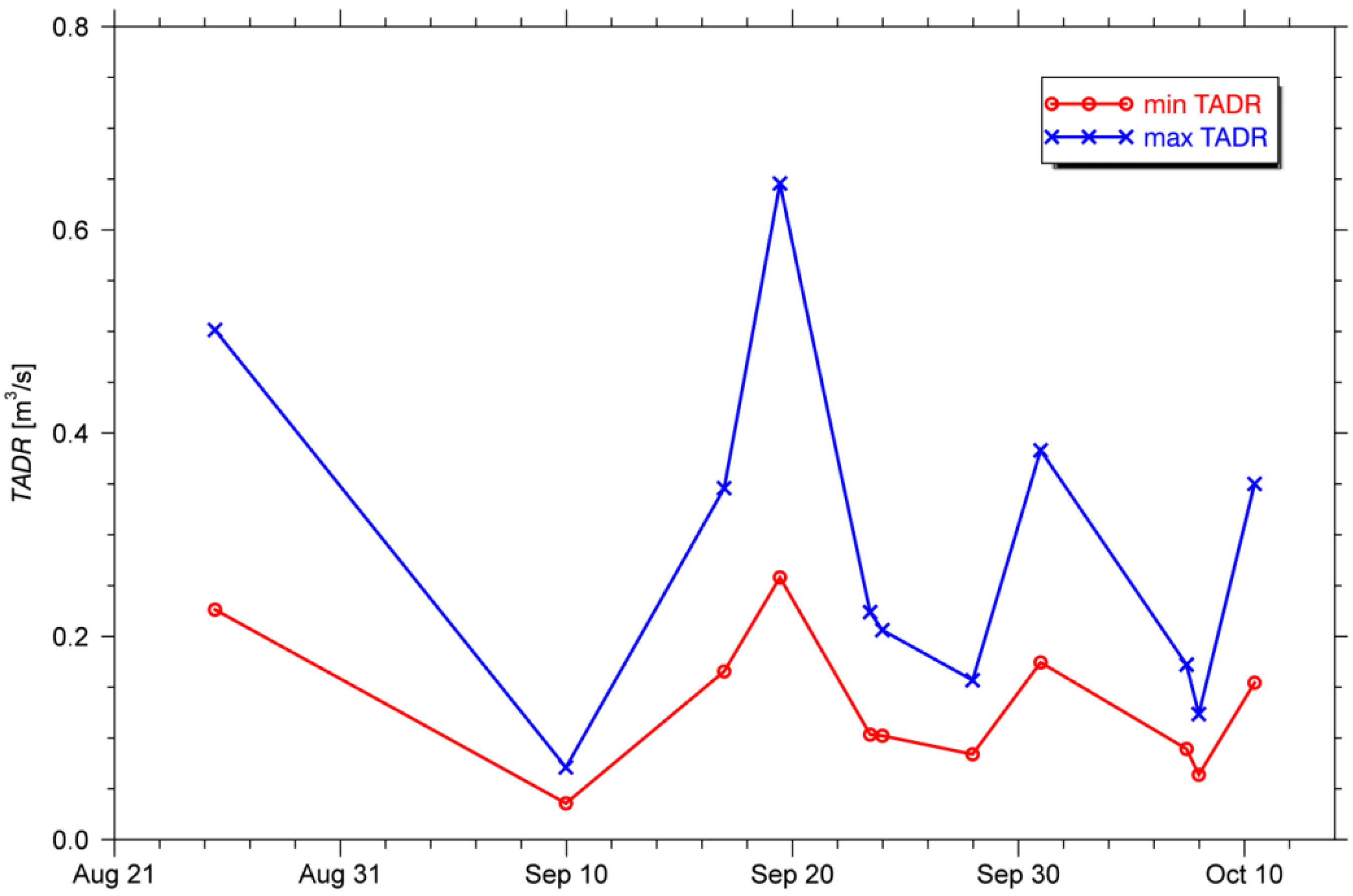
4.1. Field Observations

A team of researchers from the University of Hamburg monitored Stromboli’s activity in September 2014. Along with other instruments, we also used two cameras that covered different parts of the infrared spectrum. The cameras were used at different locations (Table 2, Figure 2). Given our cameras’ field of view (see Table 3), we selected different observation locations that provided the best possible view of the lava flows.
Table 2. Field observation metadata; point D corresponds to the observations conducted from the boat.
ABCD
Longitude15°12′49.92″ E15°12′52.12″ E15°12′48.68″ E15°12′15″ E
Latitude38°48′18.58″ N38°48′13.52″ N38°48′26.68″ N38°48′59″ N
Observer elevation293 m372 m178 m0 m
Target mean elevation600 m700 m300 m500 m
Date (September 2014)10, 12, 15,171618–2420 (boat)
Mean dist. from the lava flow1100 m1100 m850 m2200 m
SWIR transmittance -0.750.80-
MIR transmittance0.820.820.870.57
TIR transmittance0.700.700.750.35
Figure 2. Points represent the position (Table 2) of the effusive vent and the observation points where the thermal cameras were placed (see Table 3). The polygon shows the location of the lava flow on 19 September 2014 at 7:40 p.m. Please note that this is a perspective view from North to South.
Remotesensing 07 15876 g002
The best view came from a boat (point D in Table 2) off the Sciara del Fuco, however, the observations were not easy as the high waves swayed the boat causing inconvenient observation conditions (e.g., focusing issues). In the end most of the observations were conducted from an easy to reach point on the eastern flank of the Sciara del Fuoco (point C in Table 2).
Table 3. Main characteristics of thermal cameras.
Infratec ImageIRInfratec VarioCam HR
Spectral range2.0–5.5 μm7.5–14.0 μm
Central wavelengthsfilter 1: 2.4 μm, filter 2: 3.9 μm10.3 μm
Detector typeCooled InSB FPAUncooled micro bolometer FPA
Number of pixels640 × 512640 × 480
Temperature res. At 303 K0.02 K0.03 K
Accuracy±1%±1%
Dynamic range16 bit16 bit
Lenses focal length25 mm30 mm
Field of View21.7° × 17.5°30° × 23°
The cameras we used provided observations at different wavelengths. The first camera (Infratec VarioCam HR) measured irradiation in the TIR spectrum, while the second one (Infratec ImageIR) measured irradiation in the short-wave infrared (SWIR) and MIR spectrum. The cameras’ characteristics can be found in Table 3.
The evolution of the volcano’s activity during our field observations is documented in Table 4. The activity changed constantly: we observed several prolongations of lava fronts and fluctuations in the maximum detected temperatures, which varied by 100s of K. The most important were the movements of the lava front down the slope (Figure 3). For instance, if lava moves down the slope at ~1 m/s (Table 4, 18 September) and we assume that the average lava front is ~10 m wide and ~0.5 m high, this yields an instantaneous discharge rate of ~5 m3/s. This value cannot be compared to satellite observations, as they present a value that is averaged over a longer time period than the field observations. In addition, lava flows in short pulses cannot be observed by satellites.
Figure 3. The lava front movement between 12:09 and 12:12 on 18 September 2014 was observed with an Infratec Image IR camera (3.9 µm filter). At a distance of 850 m from the lava, the images cover a field of view measuring 326 × 261 m. The arrows point to the lava front, which moved 220 m down the slope in 3 min (see Table 4).
Remotesensing 07 15876 g003
Table 4. Log of field observations; please note that we also used a 2.4 μm filter on the Image IR camera, however the atmosphere interfered significantly with this band as it lies on the edge of the atmospheric window. Thus the filter was not used in the quantitative analysis.
Date & TimeMaximal T (K) inRemarks
TIRMIRSWIR
2014/09/10; 17:45699//We could observe the area close to the vent with T > 670 K. Mid-flow was out of sight. The lowest part was visible, but significantly cooler with T ~430 K.
2014/09/12; 10:30–13:00767//We could observe the area close to the vent with T ~750 K. T dropped between 10:30 and 10:40. First it dropped to 670 K and then it kept cooling, but remained above 570 K
2014/09/15; 16:20–17:00733961/We could observe the area close to the vent with T ~950 K (in MIR). First simultaneous observations in MIT and TIR band.
2014/09/16; 10:30–11:20758923806Only the area close to the vent was visible. First observations with SWIR filter.
2014/09/17; 13:30617//We could observe only the area just below the vent, but not the vent itself.
2014/09/17; 15:40680//We could observe the entire area with the exception of the vent. Considering the temperatures, it is likely that fresh lava remained under the crust.
2014/09/18; 12:05–12:50680728/The lava front extended between 12:09 and 12:12; it progressed by 220 m in 3 min (Figure 3). This was accompanied by a flow front brecciating and collapsing down the slope, with rocks having temperatures between 500 and 700 K and rolling down with velocities ~10 m/s.
2014/09/19; 10:55–11:35892//The observed part of the flow reached T > 770 K (at 11:07), but the lava front did not advance down the slope. At 11:10, it started to cool down to 570 K. At 11:28, it heated up again and some material broke out for 10 s.
2014/09/20; 15:50668//Short observation; we could observe only the lower part of the flow.
2014/09/20; 19:35–19:558311080 Night observations were made from a boat at a distance to vents ~2.2 km. Lava front on the west side moved for 120 m in 5 min.
2014/09/20; 23:25–23:35573751829Night observations; lava front was high on the slope.
2014/09/21; 14:40–15:00 739Observations in SWIR exposed significant degassing.
2014/09/21; 15:10-15:25535//The entire flow was visible below the vent.
2014/09/21; 15:28–15:38502735/Observations of the crater area revealed visible explosions shooting material up to 50 m above the terrain.
2014/09/21; 15:40–16:40529702/Lava front advanced three times: the first pulse was weak; the second one was stronger—it moved the lava front 240 m down the slope in 5 min; the third pulse moved the lava front with the same velocity over the same path as the second event.
2014/09/22; 11:20–12:40543737/Low temperatures and low activity with some rock-fall and some minor movements of the lava front.
2014/09/23; 10:30–10:458721112977High temperatures were observed high on the slope and not on the lowest lava front. Some intense degassing (no ash) was visible above the crater.
2014/09/24; 16:10652 Although the temperatures were relatively low, the lava flow almost reached the sea.
Despite the problems of observations from the boat (Figure 4), the coverage of the lava flows was greatly superior to the observations from the eastern flank of the volcano. Those images allowed us to directly estimate VRP and TADR, because we were able to observe most of the entire lava flow. The observations were corrected for the geometry (the pixel area was underestimated due to the low viewing angle), atmospheric effects, and emissivity. Similar as in our satellite data processing, we assumed a flat emissivity of 0.95. Transmittances (Table 2) were estimated using MODTRAN [36] at which a mid-latitude summer model was used. These parameters were entered into Irbis 3 plus thermography software, which was used to correct the temperatures. Temperatures observed with the VarioCam camera (TIR spectrum) are significantly lower than temperatures measured with the ImageIR camera using a narrow band filter centered at 3.9 μm (Figure 4). The difference between the two datasets can be partially attributed to the differences in the camera resolutions (VarioCam: 1.83 m at a distance of 2200 m), which is coarser than the resolution of the ImageIR (1.32 m). However, of course, the main reason is due to the higher sensitivity of the ImageIR for fresh lava radiating through the cracks in the lava crust.
Figure 4. A comparison of the TIR and MIR observations from a boat on 20 September 2014 at 19:39:39; VarioCam data were resampled to the resolution of the ImageIR.
Remotesensing 07 15876 g004
If the temperature data from both cameras (Figure 4) are applied to Stefan-Boltzmann’s law to estimate first VRP [4,5] and then TADR, we obtain different values (Table 5). In addition, the effective temperature of the lava flow based on the dual band solution provides data for a third version of TADR. We assumed that the temperature of the lava seen in the cracks was 1273 K. The results show that most of the flow was covered by a relatively cool lava crust (400–450 K) which covered the majority of the pixel (95%–97%, in rare pixels less than 85%). For most of the flow pixels the effective temperature was around 600 K, with a maximum value of over 800 K.
Table 5. TADR based on the observations with thermal cameras on 20 September 2014 at 7:39:39 p.m.
Min TADR (m3/s)Max TADR (m3/s)
ImageIR 3.9 μm0.1890.409
VarioCam0.1900.343
Teff (dual band)0.1860.440
As expected, ImageIR temperatures yield a higher TADR than VarioCam temperatures for the min TADR as well as for the max TADR model. It is interesting that TADR estimated from the effective temperature is very similar to the ImageIR results. Although we may assume that the observations in the MIR spectrum are better suited for TADR estimation, the difference between MIR and TIR observations is still significantly smaller (~16%) than the errors between min TADR and max TADR models. Thus we may conclude that the most probable TADR during our observations from a boat was 0.31 m3/s. This value was higher than TADR estimated some hours later by TET-1 (cloudy situation), but the simultaneous field observations at the time of the TET-1 overpass showed that the lava front retreated significantly up the slope. This means that the activity decreased between our observations from the boat (at 19:35–19:55; Table 5) and the TET observations (at 23:25–23:35).

4.2. TET-1 Observations

Figure 5 shows 18 processed datasets (MIR band temperature corrected for emissivity and atmospheric effects). Another 9 datasets were acquired but these situations were mostly too cloudy to be used. The presented data were atmospherically corrected and shows temperatures.
Figure 5. TET-1 MIR temperature corrected for emissivity and atmospheric effects over Stromboli. Lava flows appear in red-orange-yellow colors while the background appears in black-blue-green colors.
Remotesensing 07 15876 g005
The lowest temperature was detected on clouds during the night (see Figure 5 for the date 2 September 2014). Clouds seem to be warmer during the daytime, which is a consequence of the reflected solar irradiance. The Tyrrhenian Sea around the island had a relatively constant temperature of approximately 27 °C in August and September, indicating merely small diurnal variations, thus it appears as a constant background. The island itself shows significantly higher diurnal deviations (~15 °C) with maximum temperatures of over 30 °C. Most prominent in Figure 5 are the lava flows, which stand out with their red-orange-yellow colors on most scenes. It is obvious that the number of pixels associated with the high temperature anomaly varies significantly, e.g., the number of pixels covering the active lava flow reduces to a single pixel on 5 September 2014.
Two main reasons influenced this high variability. Firstly, the cloud coverage varied significantly from scene to scene, for instance a hotspot was detected on 2 September 2014, but its quantification is likely to contain a huge error due to cloud coverage. Therefore, images from 2, 5, 12, 20, 26 and 30 September were not further considered. In addition, the morning overpass on 16 September also had problems in the TIR channel, thus, it was not processed either. The second reason is the highly variable lava production rate of the volcano. Most scenes clearly reveal two separate lava flows. Sometimes they converge into one on their way to the sea. The spatial resolution of TET-1 data are still too coarse to identify the exact position of the vent or exact length of each flow. The longest flow identified (25 August 2014) is estimated to 6 TET-1 pixels, which is, considering that the first and the last pixel are not fully covered by the flow, ~800 m (map and not slope distance). Considering the average slope of the Sciara del Fuoco is 37°, the elevation difference between the effusive vent and the lava front was 600 m. As the vent was located 650 m a.s.l., the lava front almost reached the sea.
Figure 6 shows the estimated TADR based on TET-1 data. Instead of producing a single value per scene, we show the minimum and maximum estimates. The reason behind this lies in the poor knowledge of precise values for some parameters in Equation (7). As previously proposed [5,6,23,55], we thus provide two datasets ranging from the lowest (min TADR) to the highest possible estimate (max TADR). The used parameters are listed in Table 6.
Figure 6. Minimal and maximal values of TADR in m3/s, obtained from TET-1 data.
Remotesensing 07 15876 g006
Table 6. Input parameters for TADR estimation [23].
ParameterMin TADRMax TADR
Tamb ambient air temperature303 K
Tcore lava core temperature 1273 K
Tbase flow base temperature 773 K
k lava thermal conductivity0 W/m2/K1.5 W/m2/K
hc convective heat transfer coefficients10 W/m2/K15 W/m2/K
ρ lava density2340 kg/m32030 kg/m3
cp lava specific heat capacity1035 J/kg/K900 J/kg/K
ΔT temperature diff. between eruption and solidus temperature350 K200 K
f mass fraction of post eruption crystallization0.45
L latent crystallization heat3.5 × 105 J/m3
h thickness of thermal boundary layer1 m
In order to ignore the effect of heat conduction into the adjacent rock we used the minimum value of 0 W/m2/K in the min model for lava thermal conductivity k. The convective heat transfer coefficient hc has the greatest impact on the results. Harris et al. [23] suggested a value of ~10 W/m2/K for Stromboli, thus we used 10 W/m2/K for the min model and 15 W/m2/K for the max model.

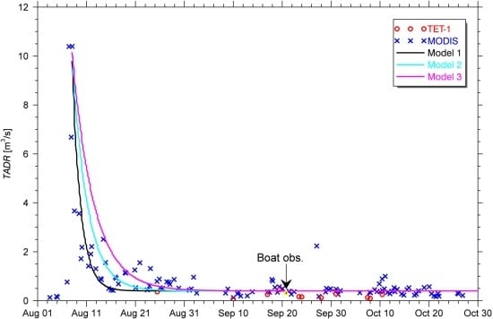
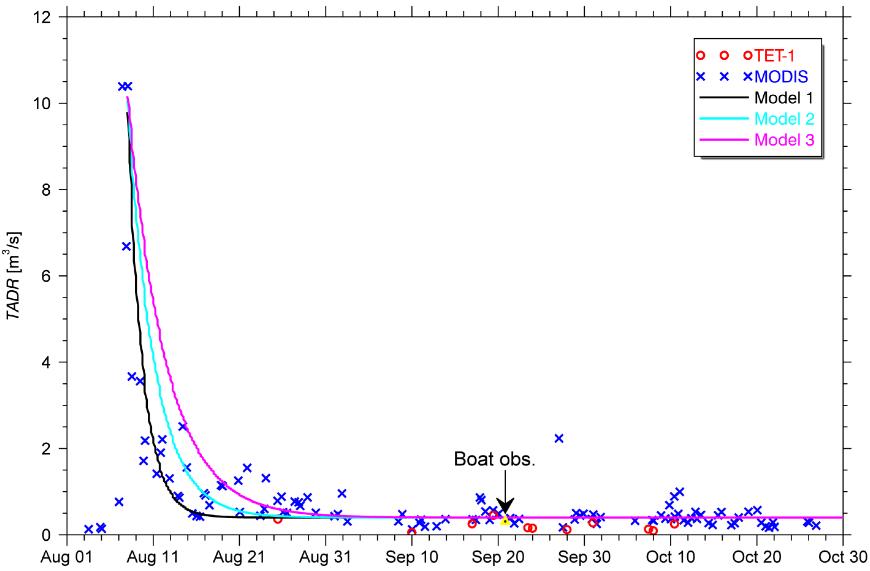
4.3. MODIS Observations

Spectral radiances for the detected thermal anomalies derived from MODIS data are archived in the MODVOLC database [21,35]. Wright and Pilger [24] suggested the use of this data to estimate the VRP with the use of Wooster’s method [58]. Figure 7 shows VRP observations from MODIS, TET-1 and one field thermal cameras (boat observations in Section 4.1).
Figure 7. VRP in MW as observed from TET-1, MODIS, and field cameras.
Remotesensing 07 15876 g007
The plot in Figure 7 is scaled in such a way that the details are also seen in the second half of eruption. However, it is impossible to see the three highest VRP values observed by MODIS at the beginning of the eruption. The maximal observed VRP was 4.2 GW. The plot shows significant fluctuations in the MODIS VRP. These are most likely the consequence of cloud coverage. In our previous work [25,26] we were dealing with uncertainties in VRP’s time series. However, we cannot use the methodology based on the Kalman filter to filter out the outliers, as we have only used the MODVOLC database, which is more convenient than processing a large number of MODIS images. The outliers were removed using a moving window analysis—if an observation was three-times smaller than the maximal VRP within the five nearest observations, this observation was considered to be affected by clouds. The filtered results (one third of situations were removed) in Figure 7 seem to be much smoother than the original time series (not shown here), but they still contain fluctuations.
MODIS data with a zenith angle greater than 50° was not further considered as well. One pixel was saturated in channel 21 at the very beginning of the eruption, thus it was assigned to contain a value of the saturation limit (radiance of 98 W/m2/µm/sr). As MODIS has a wide swath, the pixel area, which influences the kinst in the Wooster method, was also considered.
The estimation of the VRP with the use of the MODVOLC database is straightforward. However, it is impossible to estimate the effective temperature of the lava flow and the fraction of the pixel it covers. This is because the background temperature is unknown—MODVOLC only stores data for a detected anomaly but not for its vicinity. As TADR estimation using Equation (7) could not be used, we followed the radiant density approach proposed by Coppola et al. [61]. They propose that radiant density is a function of the silica content within the magma. Using their methodology, the radiant density for Stromboli, containing 50% of silica, equals 1.4 × 10⁸ J/m3 (see Section 5.2). At the start of the eruption, this corresponds to TADR of ~30 m3/s. As this value was not realistic (compared to previous eruptions) [8], we used TET-1 data to fit the radiant density (Figure 8).
Using the linear fit between TET-1 VRP and the averages of the min/max TADR, the radiant density was estimated to 4.1 × 10⁸ J/m3. This value is almost three times higher than the theoretical value suggested by Coppola et al. [61]. Two additional fits were estimated based on the scatter pattern in TET-1 data (Figure 8), but neither of them presented a good fit for the theoretical value. The estimate for MODIS TADR is given in Equation (9):
T A D R V R P 4.1 · 10 8   J m 3
Figure 8. TET-1 data shows that TADR is well correlated to VRP, allowing a linear fit of the radiant density also for MODIS.
Remotesensing 07 15876 g008
Figure 9 compares observed TADR (mean of TET-1 values in Figure 6, values derived from MODIS using Equation (9), and boat observations) and model outputs (see Section 5.1). Contrary to our TET-1 data the MODIS data also captured the intense beginning of the eruption with a maximum TADR of 10.4 m3/s. Some days later, the average value dropped below 1 m3/s. At the end of August, TADR was about 0.5 m3/s. This was also revealed by the first TET-1 data. The first half of September was relatively cloudy, thus the estimated values cannot be considered reliable (see Figure 5). Later in the month, it was possible to identify a few peaks in TET-1 and MODIS data, but the activity stagnated at TADR of 0.4 m3/s. Such evolution is in line with the classical magma discharge models with rapid waxing and slowly waning flow [62,63].
MODIS data are available for the whole eruption, thus we can estimate the total volume of the discharged lava. The mean output rate is 0.87 m3/s, which is more than the estimates for previous eruptions [5]. If we multiply this value by the duration of the eruption (6 August–13 November; 99 days), the total value of the erupted material equals 7.4 × 10⁶ m3. Considering that it is highly likely that the MODIS data still contain some data affected by the clouds, this is a lower estimate for the total erupted volume.
Figure 9. TADR in m3/s for observations along with the results of model calculations. The geometry of the model is shown in Figure 10 and the parameter varied is the length L (model 1 L = 20 m, model 2: L = 35 m, model 3, L = 50 m) of the tube feeding the flow at the vent. For more details on the model calculation, see Section 5.1.
Remotesensing 07 15876 g009

5. Discussion

In order to verify our results presented above, we (1) explain the waning mass flux with the use of a theoretical model; and (2) critically evaluate the TET-1 data.

5.1. Simple Model for Waning Mass Flux

In Figure 9, we compare our observations with the results of some model calculations for the temporal variation of the mass flux during a flank eruption at Stromboli. Model outputs are based on a very elegant and yet simple model developed by Ripepe et al. [8]. They used a multidisciplinary data set consisting of seismic, infrared and deformation data with which they modeled TADR as a function of time. Our model embodies their geometry (see Figure 10) in which the system is divided into an upper and a lower reservoir flux, both of which contribute to TADR out of the vent on the side of the volcano. The flux from the upper reservoir is TADRU, while the long term flux from the lower reservoir is TADRL = 0.4 m3/s, which is slightly higher than the flux determined by Allard et al. [64], whose estimate is 0.3 m3/s. The flux through the tube located on the side of the main plumbing system is described by the Poiseuille flow.
Figure 10. Geometry of the model for the eruptive flux from an ephemeral vent at Stromboli volcano. The model has been taken from Ripepe et al. [8].
Remotesensing 07 15876 g010
T A D R ( t ) = a 4 8 · η · L · Δ P ( t ) = T A D R U + T A D R L
where a represents the radius of the tube feeding the flow from the ephemeral vent, η represents the viscosity of the magma and L represents the length of the tube that feeds the flow. The driving pressure of the flow equals the magmastatic pressure:
Δ P ( t ) = ρ · g · h ( t )
Please note that we have neglected the difference in the atmospheric pressure in this model due to the height difference between the top of the upper reservoir and the tube outlet; the magmastatic pressure is the only driving pressure. ρ is the density of the magma containing bubbles, g is the acceleration as a result of gravity while h(t) describes the magma level due to the slow emptying of the upper reservoir of size VR(t) (for details, see Ripepe et al. [8]):
V R ( t ) = h ( t ) · A 0
where A0 is the base of the reservoir, which can be represented by a shallow cylindrical plumbing system immediately above the effusive vent (for details see Ripepe et al., [8]). From our measurements, the initial eruptive flux TADR0 at the beginning of the effusive period is known. Using Equation (10), this allows us to determine the initial height h0 of the upper reservoir.
Δ P 0 = 8 · η · L · T A D R 0 a 4 = ρ · g · h 0 h 0 = 1 ρ · g · ( 8 · η · L · T A D R 0 a 4 )
h(t) can now b e determined from the slowly emptying upper reservoir
V R ( t ) = V 0 0 t ( T A D R T A D R L ) d t
with V0 being the initial magma volume in the reservoir (h0·A0). Since TADRL is assumed to be a constant flux, Equation (14) can be rewritten
V R ( t ) = V 0 T A D R L · t + 0 t T A D R ( t ) d t
From which h(t) can be calculated
h ( t ) = h 0 1 A 0 · ( 0 t T A D R ( t ) d t T A D R L · t ) .
When we combine Equations (10), (11), and (16), we find:
T A D R ( t ) = a 4 8 · η · L · [ h 0 1 A 0 · ( 0 t T A D R ( t ) d t T A D R L · t ) ] ,
which can be solved numerically for TADR(t). We used the initial flux TADR0 = 10.4 m3/s (Section 4.3), magma density ρ = 2000 kg/m3, tube diameter a = 1.5 m, viscosity η = 104 Pa s, and the area of the reservoir A0 = 3 × 10⁴ m2. Except for the length of the tube L and the lower flux TADRL, all parameters were taken from Ripepe et al. [8]. L was taken to be smaller, for during the 2014 eruptive period the vent was located at 650 m a.s.l., while during the 2007 effusive period it was located at 400 m a.s.l.. Three values for the tube length L feeding the vent were used (see Figure 9). For these three models, the initial height h0 was estimated to 48 m (model 1, L = 20 m), 86 m (model 2, L = 35 m), and 125 m (model 3, L =50 m), respectively. Model 2 fits the true elevation difference between the crater terrace and the effusive vent better than the other two. Models 1 and 2 fit the initial decrease of the effusion rate quite well but all models fail to capture the slightly higher effusion rates between 21 August and 4 September.

5.2. Added Value of TET-1 Data

Monitoring of effusive volcanic activity at high temporal and high spatial resolution has not been possible until TET-1 became operational. TET-1 does not saturate in the MIR channel making it much more useful than other high resolution instruments like Landsat ETM+ or ASTER that tend to saturate in the case of intensive volcanic activity. Once BIROS is launched, the FireBird constellation will be able to provide data at least once per 3 days above the Equator.
Figure 11 shows the analysis of lava flows observed by TET-1. Using the dual band method (Equation (1)), we estimated the effective temperature and the area covered by lava flows as well as their length. Please note, that the lengths are upper estimates, as we did not consider the point spread function of the instrument. A comparison between the TET-1 values and the observations from the boat reveal that the temperature and length of the flows are in a good agreement. However, the estimated areas of lava flows from the TET-1 and boat observations do not match on 19 September 2014. There are two possible explanations for this observation.
(1) The observations of the flow from the boat simply did not capture the whole flow because of the low viewing angle. Looking at Figure 4 one can see that the lava flow seems to be coming from the left before it becomes visible to the camera. Field observations from a higher elevation on the slope show a big bulge of colder lava, which was built during the eruption. This bulge might hinder a direct view from the sea onto this large part of the flow. Above the bulge, the flow continued to the vent that is also not visible in Figure 4. This could well explain at least some of the differences detected between the boat and space based observations.
(2) Comparing this one with other situations in Figure 5, we can see relatively cool lava flows covering a similar number of pixels as in other situations. Thus, the reasons of such an extreme large flow area must be related to the numerical solution of the dual band method.
Figure 11. Analysis of the effective temperature, area and length of lava flows from TET-1 data; see Table 7 for exact values.
Remotesensing 07 15876 g011
In Table 7 we list the values of estimated temperature, area, and VRP computed with (a) dual band method; and (b) Wooster’s method for the cloud-free TET-1 data. Especially interesting is the comparison between both VRP results. We can see some differences, especially for the situation discussed above and for 27 September 2014. The mean dual band VRP value for the 11 datasets is 96 MW, for Wooster’s method VRP the mean value is 115 MW. Some of these differences can be ascribed to some steps in the processing chain. It is especially interesting to see that Wooster’s method, which results fits well with MODIS data (Figure 7), produces in general higher values. This deviation will be addressed in the future, as TET-1 data will be available for several volcanoes.
Table 7. Temperature (T), area (A), and volcanic radiative power estimated using dual band (VRPBD) and Wooster’s method (VRPW) for TET-1 cloud free data.
Date/TimeT (K)A (Ha)VRPDB (MV)VRPW (MW)
2014/08/25 10:495723.2182187
2014/09/09 23:306720.22336
2014/09/16 23:325871.7105155
2014/09/19 10:465047.4238167
2014/09/23 10:335831.37890
2014/09/23 23:346010.752102
2014/09/27 23:219660.16294
2014/09/30 23:345412.6115150
2014/10/07 10:337240.34995
2014/10/07 23:336980.23268
2014/10/10 10:455392.7117124
In the past, the dual band method has been criticized for yielding unrealistic results [45,46,47,48,49]. Compared to older satellite instruments (for instance MODIS), TET-1 has an improved spatial resolution. Older instruments usually cover such a large pixel area that the assumption of only two endmembers in a pixel (hotspot and background) is unrealistic. This is nicely demonstrated by the fact that TET-1 can also see the separate flows on Stromboli, while in the MODIS images the whole flow covers only one pixel . This prevents a more detailed analysis on the extent of the lava flow from MODIS data, which is extremely important for modeling the evolution of the flow as well as for hazard assessment related issues.
Applying the dual band method to the TET-1 data, which have a significantly higher spatial resolution than MODIS data, makes the solution of the dual band method much more reliable, as the two endmember model is better suited for smaller pixels. The problem is that TET-1 does not perform at the same retrieval rate as MODIS, because of its limited on-board data storage and its narrow swath (~10 times narrower than MODIS). Thus, MODIS-like instruments are still indispensable for operational use. An elegant way to estimate TADR from MODIS data is to apply the radiant density approach [61] to the MODVOLC database. Equation (18) provides the estimate of radiant density, where XSiO2 is the silica content (wt%) of the erupted lava [61].
c r a d = 6.45 · 10 25 · ( X S i O 2 ) 10.4
By applying the radiant density approach for Stromboli, whose minimal silica content is 50 wt% [61], the radiant density is estimated to 1.4 × 10⁸ J/m3. With upper estimated silica content for Stromboli of 55 wt%, the radiant density is even lower. Using these two estimates, TADR in the beginning of the eruption would be ~3 and ~10 times larger than our TADR at the beginning of the eruption (10.4 m3/s). Such high TADR was not modeled nor observed during 2007 eruption at Stromboli: maximum observed TADR during the 2007 eruption was 23 m3/s [8]. In addition, the here estimated radiant density is more comparable to the corresponding values of max and min TADR model for June 2003 eruption [5] than to the theoretical estimate based on Equation (18). Thus, we conclude that it is necessary to calibrate the approach suggested by Coppola et al. [61] with high resolution unsaturated data provided by TET-1. In the future, it should be possible to refine Equation (18) [61], but it would be necessary to monitor several eruptions, also during their waxing flow.

6. Conclusions

This is the first time a long term observation of thermal radiance at an active volcano was performed using a small satellite, in this case TET-1, which provides unsaturated data at high spatial resolution in MIR and TIR bands. TET-1 data were not available for the whole eruption period, but we were still able to retrieve TADR with a combined use of TET-1 and MODIS data. The results correspond well to field observation data using a combination of cameras operating in MIR and TIR bands. The mean output rate for the entire eruption equals 0.87 m3/s, which is higher than in the 2002–2003 eruption, but less than in the 2007 eruption. These differences can be partially explained by the model based on Poiseuille flow, where the pivotal role belongs to the height difference between the crater terrace and the effusive vent, i.e., the driving magmastatic pressure. During the three-month-long eruption Stromboli erupted an estimated volume of 7.4 × 10⁶ m3 of material.

Acknowledgments

This research has been supported by a grant from the German Science Foundation (DFG), number ZA659/1-1. The TET-1 data are courtesy of German Aerospace Centre (DLR). We would also like to thank the members of the University of Hamburg who took part in the Stromboli 2014 campaign, especially Leonie Pick, who performed excellent work during the preparation for the campaign, and Jost van der Lieth, who supported us with GPS data. Finally, we would also like to thank Dieter Örtel, Olaf Frauenberger, and Carsten Paproth for their contributions in the debate on the TET-1 point spread function.

Author Contributions

Klemen Zakšek designed the study and analyzed the field and satellite data. Matthias Hort organized the field campaign and analyzed the results of the theoretical model. Eckehard Lorenz prepared the satellite data. All authors have read and edited the manuscript.

Conflicts of Interest

The authors declare no conflict of interest.

References

  1. Blackburn, E.A.; Wilson, L.; Sparks, R.S.J. Mechanisms and dynamics of strombolian activity. J. Geol. Soc. 1976, 132, 429–440. [Google Scholar] [CrossRef]
  2. Chouet, B.; Hamisevicz, N.; McGetchin, T.R. Photoballistics of volcanic jet activity at Stromboli, Italy. J. Geophys. Res. 1974, 79, 4961–4976. [Google Scholar] [CrossRef]
  3. De Fino, M.; la Volpe, L.; Falsaperla, S.; Frazzetta, G.; Neri, G. The Stromboli eruption of December 6, 1985–April 25, 1986: Volcanological, petrological and seismological data. Rend. Soc. Ital. Miner. Pet. 1988, 43, 1021–1038. [Google Scholar]
  4. Calvari, S.; Spampinato, L.; Lodato, L.; Harris, A.J.L.; Patrick, M.R.; Dehn, J.; Burton, M.R.; Andronico, D. Chronology and complex volcanic processes during the 2002–2003 flank eruption at Stromboli volcano (Italy) reconstructed from direct observations and surveys with a handheld thermal camera. J. Geophys. Res. Solid Earth 2005, 110. [Google Scholar] [CrossRef]
  5. Harris, A.; Dehn, J.; Patrick, M.; Calvari, S.; Ripepe, M.; Lodato, L. Lava effusion rates from hand-held thermal infrared imagery: An example from the June 2003 effusive activity at Stromboli. Bull. Volcanol. 2005, 68, 107–117. [Google Scholar] [CrossRef]
  6. Calvari, S.; Lodato, L.; Steffke, A.; Cristaldi, A.; Harris, A.J.L.; Spampinato, L.; Boschi, E. The 2007 Stromboli eruption: Event chronology and effusion rates using thermal infrared data. J. Geophys. Res. Solid Earth 2010, 115. [Google Scholar] [CrossRef] [Green Version]
  7. Ripepe, M.; Delle Donne, D.; Lacanna, G.; Marchetti, E.; Ulivieri, G. The onset of the 2007 Stromboli effusive eruption recorded by an integrated geophysical network. J. Volcanol. Geotherm. Res. 2009, 182, 131–136. [Google Scholar] [CrossRef]
  8. Ripepe, M.; Donne, D.D.; Genco, R.; Maggio, G.; Pistolesi, M.; Marchetti, E.; Lacanna, G.; Ulivieri, G.; Poggi, P. Volcano seismicity and ground deformation unveil the gravity-driven magma discharge dynamics of a volcanic eruption. Nat. Commun. 2015, 6. [Google Scholar] [CrossRef] [PubMed]
  9. Tinti, S.; Maramai, A.; Armigliato, A.; Graziani, L.; Manucci, A.; Pagnoni, G.; Zaniboni, F. Observations of physical effects from tsunamis of 30 December 2002 at Stromboli volcano, southern Italy. Bull. Volcanol. 2005, 68, 450–461. [Google Scholar] [CrossRef]
  10. Tinti, S.; Pagnoni, G.; Zaniboni, F.; Bortolucci, E. Tsunami generation in Stromboli island and impact on the south-east Tyrrhenian coasts. Nat. Hazards Earth Syst. Sci. 2003, 3, 299–309. [Google Scholar] [CrossRef]
  11. Di Traglia, F.; Battaglia, M.; Nolesini, T.; Lagomarsino, D.; Casagli, N. Shifts in the eruptive styles at Stromboli in 2010–2014 revealed by ground-based InSAR data. Sci. Rep. 2015, 5. [Google Scholar] [CrossRef] [PubMed]
  12. Rizzo, A.L.; Federico, C.; Inguaggiato, S.; Sollami, A.; Tantillo, M.; Vita, F.; Bellomo, S.; Longo, M.; Grassa, F.; et al. The 2014 effusive eruption at Stromboli volcano (Italy): Inferences from soil CO2 flux and 3He/4He ratio in thermal waters. Geophys. Res. Lett. 2015, 42. [Google Scholar] [CrossRef]
  13. Simkin, T.; Siebert, L. Volcanoes of the World: A Regional Directory, Gazetteer, and Chronology of Volcanism during the Last 10,000 Years; Geoscience Press: Tucson, AZ, USA, 1994. [Google Scholar]
  14. Oppenheimer, C.; Francis, P. Remote sensing of heat, lava and fumarole emissions from Erta ’Ale volcano, Ethiopia. Int. J. Remote Sens. 1997, 18, 1661–1692. [Google Scholar] [CrossRef]
  15. Coppola, D.; Piscopo, D.; Staudacher, T.; Cigolini, C. Lava discharge rate and effusive pattern at Piton de la Fournaise from MODIS data. J. Volcanol. Geotherm. Res. 2009, 184, 174–192. [Google Scholar] [CrossRef]
  16. Dehn, J.; Dean, K.; Engle, K. Thermal monitoring of North Pacific volcanoes from space. Geology 2000, 28, 755–758. [Google Scholar] [CrossRef]
  17. Harris, A.J.L.; Swabey, S.E.J.; Higgins, J. Automated thresholding of active lavas using AVHRR—Data. Int. J. Remote Sens. 1995, 16, 3681–3686. [Google Scholar] [CrossRef]
  18. Lombardo, V.; Buongiorno, M.; Amici, S. Characterization of volcanic thermal anomalies by means of sub-pixel temperature distribution analysis. Bull. Volcanol. 2006, 68, 641–651. [Google Scholar] [CrossRef]
  19. Pergola, N.; Marchese, F.; Tramutoli, V. Automated detection of thermal features of active volcanoes by means of infrared AVHRR records. Remote Sens. Environ. 2004, 93, 311–327. [Google Scholar] [CrossRef]
  20. Rothery, D.A.; Francis, P.W.; Wood, C.A. Volcano monitoring using short wavelength infrared data from satellites. J. Geophys. Res. 1988, 93, 7993–8008. [Google Scholar] [CrossRef]
  21. Wright, R.; Flynn, L.; Garbeil, H.; Harris, A.; Pilger, E. Automated volcanic eruption detection using MODIS. Remote Sens. Environ. 2002, 82, 135–155. [Google Scholar] [CrossRef] [Green Version]
  22. Davies, A.G.; Calkins, J.; Scharenbroich, L.; Vaughan, R.G.; Wright, R.; Kyle, P.; Castańo, R.; Chien, S.; Tran, D. Multi-instrument remote and in situ observations of the Erebus Volcano (Antarctica) lava lake in 2005: A comparison with the Pele lava lake on the jovian moon Io. J. Volcanol. Geotherm. Res. 2008, 177, 705–724. [Google Scholar] [CrossRef]
  23. Harris, A.J.L.; Dehn, J.; Calvari, S. Lava effusion rate definition and measurement: A review. Bull. Volcanol. 2007, 70, 1–22. [Google Scholar] [CrossRef]
  24. Wright, R.; Pilger, E. Radiant flux from Earth’s subaerially erupting volcanoes. Int. J. Remote Sens. 2008, 29, 6443–6466. [Google Scholar] [CrossRef]
  25. Zakšek, K.; Shirzaei, M.; Hort, M. Constraining the uncertainties of volcano thermal anomaly monitoring using a Kalman filter technique. Geol. Soc. Lond. Spec. Publ. 2013, 380, 137–160. [Google Scholar] [CrossRef]
  26. Zakšek, K.; Pick, L.; Shirzaei, M.; Hort, M. Thermal monitoring of volcanic effusive activity: The uncertainties and outlier detection. Geol. Soc. Lond. Spec. Publ. 2015, 426. [Google Scholar] [CrossRef]
  27. Lombardo, V.; Musacchio, M.; Buongiorno, M.F. Error analysis of subpixel lava temperature measurements using infrared remotely sensed data. Geophys. J. Int. 2012, 191, 112–125. [Google Scholar] [CrossRef]
  28. ESA SMO FuegoTec Programme—GSP. Available online: http://gsp.esa.int/document-view/-/wcl/wlGiHTp4j7JC/10192/smo-fuegotec-programme (accessed on 11 August 2015).
  29. Schroeder, W.; Oliva, P.; Giglio, L.; Csiszar, I.A. The New VIIRS 375 m active fire detection data product: Algorithm description and initial assessment. Remote Sens. Environ. 2014, 143, 85–96. [Google Scholar] [CrossRef]
  30. Lorenz, E.; Mitchell, S.; Säuberlich, T.; Paproth, C.; Halle, W.; Frauenberger, O. Remote sensing of high temperature events by the FireBird mission. ISPRS Int. Arch. Photogramm. Remote Sens. Spat. Inf. Sci. 2015, XL-7/W3, 461–467. [Google Scholar] [CrossRef]
  31. Briess, K.; Jahn, H.; Lorenz, E.; Oertel, D.; Skrbek, W.; Zhukov, B. Fire recognition potential of the bi-spectral Infrared Detection (BIRD) satellite. Int. J. Remote Sens. 2003, 24, 865–872. [Google Scholar] [CrossRef]
  32. Fischer, C.; Klein, D.; Kerr, G.; Stein, E.; Lorenz, E.; Frauenberger, O.; Borg, E. Data validation and case studies using the TET-1 Thermal Infrared Satellite System. ISPRS Int. Arch. Photogramm. Remote Sens. Spat. Inf. Sci. 2015, XL-7/W3, 1177–1182. [Google Scholar] [CrossRef]
  33. Jahn, H.; Reulke, R. Staggered Line Arrays in Pushbroom Cameras: Theory and Application. Available online: http://elib.dlr.de/18149/ (accessed on 21 November 2015).
  34. DLR Firebird—Data Access and Products. Available online: http://www.dlr.de/firebird/en/desktopdefault.aspx/tabid-9090/17974_read-42458/ (accessed on 27 October 2015).
  35. Wright, R.; Flynn, L.P.; Garbeil, H.; Harris, A.J.L.; Pilger, E. MODVOLC: Near-real-time thermal monitoring of global volcanism. J. Volcanol. Geotherm. Res. 2004, 135, 29–49. [Google Scholar] [CrossRef]
  36. Berk, A.; Anderson, G.P.; Acharya, P.K.; Bernstein, L.S.; Muratov, L.; Lee, J.; Fox, M.; Adler-Golden, S.M.; Chetwynd, J.H., Jr.; Hoke, M.L.; et al. MODTRAN5: 2006 update. SPIE Proc. 2006, 6233. [Google Scholar] [CrossRef]
  37. Harris, A. Thermal Remote Sensing of Active Volcanoes: A User’s Manual; Cambridge University Press: Cambridge, UK, 2013. [Google Scholar]
  38. Zhukov, B.; Lorenz, E.; Oertel, D.; Wooster, M.; Roberts, G. Spaceborne detection and characterization of fires during the bi-spectral infrared detection (BIRD) experimental small satellite mission (2001-2004). Remote Sens. Environ. 2006, 100, 29–51. [Google Scholar] [CrossRef]
  39. Lucy, L.B. An iterative technique for the rectification of observed distributions. Astron. J. 1974, 79, 745–749. [Google Scholar] [CrossRef]
  40. Richardson, W.H. Bayesian-based iterative method of image restoration. J. Opt. Soc. Am. 1972, 62, 55–59. [Google Scholar] [CrossRef]
  41. Duda, R.O.; Hart, P.E. Pattern Classification and Scene Analysis; John Willey & Sons: New York, NY, USA, 1973. [Google Scholar]
  42. Xie, H.; Hicks, N.; Randy Keller, G.; Huang, H.; Kreinovich, V. An IDL/ENVI implementation of the FFT-based algorithm for automatic image registration. Comput. Geosci. 2003, 29, 1045–1055. [Google Scholar] [CrossRef]
  43. Steffke, A.; Harris, A. A review of algorithms for detecting volcanic hot spots in satellite infrared data. Bull. Volcanol. 2011, 73, 1109–1137. [Google Scholar] [CrossRef]
  44. Dozier, J. A method for satellite identification of surface temperature fields of subpixel resolution. Remote Sens. Environ. 1981, 11, 221–229. [Google Scholar] [CrossRef]
  45. Oppenheimer, C. Thermal distributions of hot volcanic surfaces constrained using three infrared bands of remote sensing data. Geophys. Res. Lett. 1993, 20, 431–434. [Google Scholar] [CrossRef]
  46. Mouginis-Mark, P.J.; Garbeil, H.; Flament, P. Effects of viewing geometry on AVHRR observations of volcanic thermal anomalies. Remote Sens. Environ. 1994, 48, 51–60. [Google Scholar] [CrossRef]
  47. Wright, R.; Rothery, D.A.; Blake, S.; Pieri, D.C. Improved remote sensing estimates of lava flow cooling: A case study of the 1991–1993 Mount Etna eruption. J. Geophys. Res. 2000, 105, 23681–23694. [Google Scholar] [CrossRef]
  48. Lombardo, V.; Buongiorno, M.F. Lava flow thermal analysis using three infrared bands of remote-sensing imagery: A study case from Mount Etna 2001 eruption. Remote Sens. Environ. 2006, 101, 141–149. [Google Scholar] [CrossRef]
  49. Vaughan, R.G.; Keszthelyi, L.P.; Davies, A.G.; Schneider, D.J.; Jaworowski, C.; Heasler, H. Exploring the limits of identifying sub-pixel thermal features using ASTER TIR data. J. Volcanol. Geotherm. Res. 2010, 189, 225–237. [Google Scholar] [CrossRef]
  50. Giglio, L.; Kendall, J.D. Application of the Dozier retrieval to wildfire characterization: A sensitivity analysis. Remote Sens. Environ. 2001, 77, 34–49. [Google Scholar] [CrossRef]
  51. Moré, J.J. The Levenberg-Marquardt algorithm: Implementation and theory. In Numerical Analysis; Watson, G.A., Ed.; Springer: Berlin, Germany, 1978; Volume 630, pp. 105–116. [Google Scholar]
  52. Markwardt, C.B. Non-linear least squares fitting in IDL with MPFIT. In Proceedings of the Astronomical Data Analysis Software and Systems (ADASS) XVII, Québec, QC, Canada, 2–5 November 2008.
  53. Glaze, L.; Francis, P.W.; Rothery, D.A. Measuring thermal budgets of active volcanoes by satellite remote sensing. Nature 1989, 338, 144–146. [Google Scholar] [CrossRef]
  54. Harris, A.J.L.; Blake, S.; Rothery, D.A.; Stevens, N.F. A chronology of the 1991 to 1993 Mount Etna eruption using advanced very high resolution radiometer data: Implications for real-time thermal volcano monitoring. J. Geophys. Res. 1997, 102, 7985–8003. [Google Scholar] [CrossRef]
  55. Wright, R.; Blake, S.; Harris, A.J.L.; Rothery, D.A. A simple explanation for the space-based calculation of lava eruption rates. Earth Planet. Sci. Lett. 2001, 192, 223–233. [Google Scholar] [CrossRef]
  56. Kaufman, Y.J.; Justice, C.O.; Flynn, L.P.; Kendall, J.D.; Prins, E.M.; Giglio, L.; Ward, D.E.; Menzel, W.P.; Setzer, A.W. Potential global fire monitoring from EOS-MODIS. J. Geophys. Res. 1998, 103, 32215–32238. [Google Scholar] [CrossRef]
  57. Murphy, S.W.; Oppenheimer, C.; de Souza Filho, C.R. Calculating radiant flux from thermally mixed pixels using a spectral library. Remote Sens. Environ. 2014, 142, 83–94. [Google Scholar] [CrossRef]
  58. Wooster, M.J.; Zhukov, B.; Oertel, D. Fire radiative energy for quantitative study of biomass burning: Derivation from the BIRD experimental satellite and comparison to MODIS fire products. Remote Sens. Environ. 2003, 86, 83–107. [Google Scholar] [CrossRef]
  59. Pieri, D.C.; Baloga, S.M. Eruption rate, area, and length relationships for some Hawaiian lava flows. J. Volcanol. Geotherm. Res. 1986, 30, 29–45. [Google Scholar] [CrossRef]
  60. Crisp, J.; Baloga, S. Estimating eruption rates of planetary lava flows. Icarus 1990, 85, 512–515. [Google Scholar] [CrossRef]
  61. Coppola, D.; Laiolo, M.; Piscopo, D.; Cigolini, C. Rheological control on the radiant density of active lava flows and domes. J. Volcanol. Geotherm. Res. 2013, 249, 39–48. [Google Scholar] [CrossRef]
  62. Wadge, G. The variation of magma discharge during basaltic eruptions. J. Volcanol. Geotherm. Res. 1981, 11, 139–168. [Google Scholar] [CrossRef]
  63. Harris, A.; Steffke, A.; Calvari, S.; Spampinato, L. Thirty years of satellite-derived lava discharge rates at Etna: Implications for steady volumetric output. J. Geophys. Res. 2011, 116. [Google Scholar] [CrossRef]
  64. Allard, P.; Carbonnelle, J.; Métrich, N.; Loyer, H.; Zettwoog, P. Sulphur output and magma degassing budget of Stromboli volcano. Nature 1994, 368, 326–330. [Google Scholar] [CrossRef]

